Computer Simulation of Grain Growth in Three Dimensions
by the Phase Field Model and the Monte Carlo Method
Yoshihiro Suwa
1and Yoshiyuki Saito
2 1Research Center for Advanced Science and Technology, University of Tokyo, Tokyo 153-8904, Japan
2Department of Materials Science and Engineering, Waseda University, Tokyo 169-8555, Japan
Temporal evolution and morphology of grain structure in three dimensions were simulated by the phase field and the Monte Carlo simulations. In order to prevent impingement of grain of like orientation, a new algorithm was adopted for both simulations. Excluding the initial stage, the average area is found to be proportional to time in the phase field and the Monte Carlo simulations. The scaled grain size and the face number distributions become time-independent in both simulations. The scaled grain size and the face number distributions obtained by the phase field simulation are in good agreement with those by the Monte Carlo method. The nearest neighbor face correlation similar to the Aboav– Weaire relation is observed in simulated grain structures by both methods. The nearest neighbor face correlation for the phase field model is quite similar to that for the Monte Carlo method. The Allen–Cahn type equation for the phase field simulation can be derived from the master equation of the Monte Carlo Model.
(Received December 21, 2004; Accepted February 24, 2005; Published June 15, 2005)
Keywords: grain growth, phase field method, Monte Carlo method, three dimension, grain size distribution, face number distribution
1. Introduction
Control of microstructure of a polycrystalline material is one of most important factors that determines properties of the materials such as strength, toughness, electrical con-ductivity and magnetic susceptibility. Computer simulation models based classical thermodynamics and phase trans-formation theory have been successfully applied to prediction of microstructural evolutions in materials. However, inho-mogeneity in microstructure in materials affects mechanical properties such as impact and corrosive properties. The incorporation of factors which characterize spatial and temporal distributions of microstructure is essentially im-portant.
Understanding of kinetics of grain growth is essentially of fundamental importance, not only for its intrinsic interest, but also for its technological significance.1,2)Due to the difficulty
of incorporating topological features into analytical theories of grain growth directly3–5)there has been increasing interest in the use of computer simulations to study grain growth. A variety of models have been proposed during the past decades.6–14) Among these models, the Potts and phase field11–14)are the arguably the most robust and versatile and certainly the most highly developed and widely applied.
The Potts model was first proposed by Potts as a general-ization of the Ising model for simulating the critical transitions in magnetic materials with more than two degenerate states.6–12) The Potts model treats the evolution
of a nonequilibrium, discrete ensemble which populates a regular lattice. The ensemble can represent the compotition and structure of materials. In the early 1980s, when computational facilities became sufficiently inexpensive to make it readily accessible, the Potts model was applied to coarsening phenomena, namely grain growth11,12)and soap froth coarsening.15)Since then, it has been modified to study many microstructural evolution problems including nor-mal16) and abnormal grain growth,17) recrystallization,18) coarsening in two phase system, Ostwald ripening,19) and
microstructural evolution in thermal gradient.20)
Phase field model is based on the Onsager’s linear irreversible thermodynamics.21) It has been extensively
applied to simulation of temporal and spatial evolution of microstructure. This model represents temporal evolutions in the chemical, crystallographic and structural fields. In this model phase boundaries are assumed to be diffuse with finite thickness. The free energy density functional is defined to have continuous local order parameters. Time history of the whole microstructure is calculated by the temporal evolu-tions of local order parameters. In this paper, we will deal with single-phase polycrystalline materials. The polycrystal-line microstructure is described by a set of orientation field variables; 1ðrÞ; 2ðrÞ;. . .; QðrÞ. The interfacial energy of a material is related to parameters in fundamental equations of the phase field models,i.e.the gradient energy coefficient,, and a parameter in a local free energy function,.
One of the serious problem in grain growth simulation is that large discontinuous changes in the area of individual grain can occur when one grain meets and coalesces with another grain having the same orientation. In order to prevent the impingement of grain of like orientation too frequently, the large number ofQ, the total number of grain orientations, is chosen. The growth rate is inversely proportional toQ. To overcome the above problems, we proposed new algorithm22)
in which the grain number is allotted to each lattice point in the Monte Carlo simulation. In the phase field simulation initial structure is prepared in the way that grains have the same orientation are situated at a certain distance.
Kinetics, grain size and edge distribution results obtained by the phase field model are reported to be in good agreement with those by the Monte Carlo method.19) Krill and Chen
compared kinetics and topological results in grain growth in 3-dimension given by the phase field simulations with results by various simulations.23)However comparison of the phase field and the Monte Carlo results for similar condition is left unfinished problem.
In this paper, we execute simulation of grain growth in
3-Special Issue on Computer Modeling of Materials and Processes
dimensions by the phase field model and the Monte Carlo method with new algorithms in order to prevent large discontinuous changes in grain sizes. The phase field simulation results are compared with those by the Monte Carlo model. Kinetics of normal grain growth and topolog-ical results of grain structures such grain size distributions, grain face distributions simulated by both models under similar conditions are compared. With these results, we will discuss the interrelations of the master equation of the Monte Carlo simulation and continuum thermodynamic equations of interface motion.
2. Model Description
2.1 Phase field model
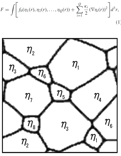
In the phase field model for the grain growth of polycrystalline materials, microstructure of polycrystalline materials is described by set of orientation field variables, 1ðrÞ; 2ðrÞ;. . .; QðrÞ, whereiðrÞ(i¼1;2;. . .;Q) are called orientation field variables that distinguish different orienta-tions of grains andQis the number of possible orientations. A schematic microstructure represented by orientation fields in 2-D is shown in Fig. 1. Within the grain labeled by 1, the absolute value for1is 1 while all otherifori6¼1is zero. Across the grain boundaries between the grain 1, and its neighbor grains, the absolute value of 1 changes continu-ously from 1 to 0. The schematic profiles of1and2across the grain boundary between the grain1and2are shown in Fig. 2. All other field variables this grain boundary having zero values. According to Cahn’s and Hilliard’s treatment,24) the total free energy functional of an inhomogeneous system is given by
F¼
Z
f0ð1ðrÞ; 2ðrÞ;. . .; QðrÞÞ þ
XQ
i¼1 i
2 ðriðrÞÞ
2
" #
d3r;
ð1Þ
where f0 is the local free energy density which is a function of orientation field variables, iðrÞ, and i is the gradient energy coefficient. The spatial and temporal evolutions of orientation field variables are described by the time-depend-ent Ginzburg–Landau equations for nonconserved order parameter.25)
@iðr;tÞ @t ¼ Li
F
iðr;tÞ; ði¼1;2;. . .;QÞ ð2Þ
where Li are the Onsager’s phenomenological coefficients. We used the Ginzburg–Landau type free energy density functional for the present simulation
f0ð1ðrÞ; 2ðrÞ;. . .; QðrÞÞ ¼
XQ
i¼1
2
2 i þ
4
4 i
þX Q
i¼1
XQ
j6¼i 2i2j;
ð3Þ
where , and are phenomenological parameters. The only requirement for f0 is that it has2Qminima with equal well depth atð1; 2;. . .; QÞ ¼ ð1;0;. . .;0Þ;ð0;1;. . .;0Þ;. . .;
ð0;0;. . .;1Þ;ð1;0;. . .;0Þ;ð0;1;. . .;0Þ;. . .;ð0;0;. . .;1Þ. Therefore, has to be greater than =2 when we assume ¼1,¼1. In order to simulate the ideal case of uniform mobility and energy, we set each order parameter equal to its absolute value, effectively restricting the available order parameter space to that containing only the Q degenerate minima of f0.13)
For the purpose of simulating the grain growth kinetics, the set of kinetic eq. (2) have to be solved numerically by discretizing them in space and time. In this paper, the Laplacian is discretized by the following equation,
r2i¼ 1 ðxÞ2
X
j
ðjiÞ; ð4Þ
wherexis the discretizing grid size, j represents the first nearest neighbors of sitei. For discretization with respect to time, we used the simple explicit Euler equation,
iðtþtÞ ¼iðtÞ þdi
dt t; ð5Þ
wheretis the time step for integration.
Fig. 1 Schematic illustration of microstructure described using orientation variables.
[image:2.595.312.539.73.222.2] [image:2.595.51.289.455.762.2]2.2 Monte Carlo simulation algorithm
In the Monte Carlo computer simulation model proposed by Exxon group,11,12) the microstructure is mapped onto
discrete lattice. To each lattice is assigned a number that corresponds to an orientation of the grain. The kinetics of grain boundary motion can be studied by counting the number of change of the orientation assigned to each lattice (reorientation trial).
In order to prevent the impingement of grain of like orientation too frequently, we proposed a new algorithm22)in
which the grain number is allotted to each lattice point. The procedure of the simulation is as follows:
. A grain number from 1 to the system size,N, is assigned to each lattice point sequentially.
. A number corresponds to an orientation of a grain is randomly assigned to each grain.
. The evolution of microstructure is tracked by the change of orientation on each lattice.
– One lattice site is selected at random
– If the lattice site belongs to grain boundary, then a new orientation is generated.
– If one of the nearest neighbor lattices has the same orientation as the newly selected grain orientation, a re-orientation trial is attempted.
– The change in energy,E, associated with the change of grain orientation is calculated.
– The re-orientation trial is accepted ifEis less than or equal to zero. If the valueEis greater than zero, the re-orientation is accepted with probability, W ¼
expðE=kBTÞ.
If the system isN, N re-orientation attempts are referred to 1 Monte Carlo step (MCS).
The change of interfacial energy accompanying re-ori-entation is a driving force of interface migration. The interfacial energy is related to the interaction energy between nearest neighbor sites. The interfacial energy is a function of the grain misorientation:
E0¼ X
hi ji
Msisj; ð6Þ
wheresiis a grain orientation which takes a value from 1 to Q. The sum is taken over nearest neighbor sites. The matrix Mi jis given by
Mi j¼Jð1i jÞ; ð7Þ
whereJ is a positive constant which sets the scale of grain boundary andi jis the Kronecker’s delta.
3. Numerical Simulation Result and Discussion
3.1 Phase field simulation
Simulation were performed on 3-dimentional lattice with size ofN¼1803and the number of orientations ofQ¼60. The lattice step sizexwas set to be 2.0 and a time steptof 0.05 was employed. All simulations were performed on the lattice systems with periodic boundary condition. In order to prevent large discontinuous change in grain size by coarsen-ing of grains havcoarsen-ing the same orientation, the nucleation sites were situated so that grains with same orientation are located at distance of a pre-set minimum distance in each phase field.
To visualize the microstructure evolution using the orienta-tion field variables, the following funcorienta-tion was defined:
’ðrr~Þ ¼X
p
i¼1
2iðrÞ; ð8Þ
which takes on a value of unity within individual grains and smaller values in the core regeions of the boundaries.13,14)If we map the value of’to a specturm of graylevels, then we obtain images like that of Fig. 3, in which the grain boundaries appears as dark regions separating individual grains. The topological properties of the latter —such as number of side, cross-sectional area, or volume— can evaluated directly by choosing a threshold value in ’ to establish the boundary positions. In this manner, it is possible to quantify the evolution of local and averaged topological grain properties during coarsening.
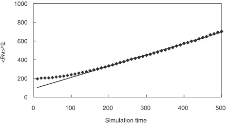
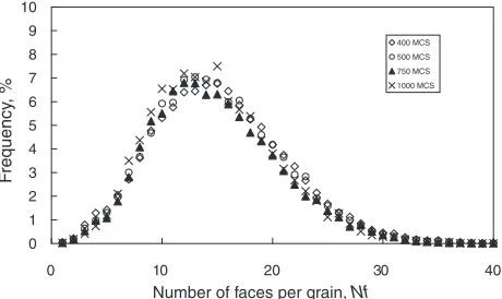
The average grain area versus time steps for the 1803 system is shown in Fig. 4. Excluding the early stage, the average area is found to be proportional to time. In order to get the grain size and grain face distributions 6 runs of simulation were performed. The scaled grain size distribution is shown in Fig. 5. After a short transient time, the grain size distribution becomes time-independent. The distribtuions of the number of face,Nf, for individual grains of the simulated microstructures is shown in Fig. 6. The distribution becomes time-invariant at the longer time. The frequency increase
Fig. 3 Microstructural evolution in180180180cells simulated by the phase field model.
0 200 400 600 800 1000
0 100 200 300 400 500
Simulation time
<Rv>^2
[image:3.595.307.546.73.242.2] [image:3.595.311.543.639.768.2]rapidly for a small number of faces and peaks at a vlaue of 12 to 14 and decays quickly. Figure 7 shows variation in the average face number with time. The initial value of 15.0 decreases with time and approaches to a constant value of about 13.7.
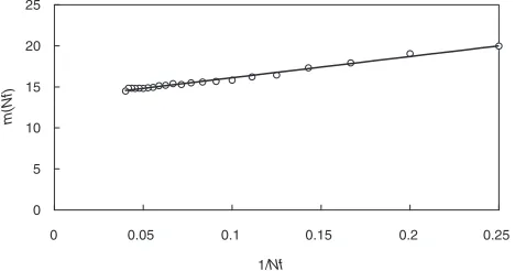
The relationship between the average number of faces of grain adjacent to an N-faced grain, mðNfÞ, and the face number in grains,Nf, is shown in Fig. 8. The linear relation equal similar to Aboav–Weaire relations26,27) is obtained betweenmðNfÞandNf as;
mðNfÞ ¼ 13:5þ25:9=Nf: ð9Þ
3.2 Monte Carlo simulation
Simulation were performed on 3-dimentional fcc like lattice with size of N¼1283. All simulations were per-formed on the lattice systems with periodic boundary condition. The number of orientation, Q, is chosen to be Q¼32. In the following simulation, the valueJ=kBTis set to
2.0. As an initial microstructure, an orientation between 1 to Qwas assigend to each grain at random. Figure 9 shows an example of temporal evolution of microstructure. The formation of grain structure is detected in the early stage of the simulation. The coasening of large grains by absorbing small grain is observed. The uniform and isotropic grain structure is obtained. The average area A, against timet, is shown in Fig. 10. The average area is found to be propor-tional to time. The average grain size,Rav, is described as a
power-law kinetics:
Rav/Bt0:5; ð10Þ
whereBis a constant which is temperature dependent. The exponent is the same as that by analytical model by Hillert.3) Figure 11 shows the variation of the scaled grain size distribution function for the simulated microstructures. The distribution function becomes time-invariant at the longer time. The distribtuions of the number of face, Nf, for 0
0.02 0.04 0.06 0.08 0.1 0.12 0.14 0.16 0.18 0.2
0 0.5 1 1.5 2 2.5
Normalized Grain Size, R/Rav
t=50 t=100 t=200 t=300 t=400
F
requency
Fig. 5 Variation in the scaled grain size distribution function with time simulated by the phase field model.
0 2 4 6 8 10 12
0 5 10 15 20 25 30 35 40
Number of faces per grain, Nf
t=50 t=100 t=200 t=300 t=400
F
requency
, %
Fig. 6 Variation in the face number distribution function with time simulated by the phase field model.
13 13.5 14 14.5 15 15.5
0 100 200 300 400 500
Simulation time
A
v
er
age n
umber of f
aces
Fig. 7 Variation in the average face number with time simulated b the phase field model.
0 5 10 15 20 25
0 0.05 0.1 0.15 0.2 0.25
1/Nf
m(Nf)
Fig. 8 Relation between the average number of faces of neighbor of N-face grain,mðNfÞand the face number,Nfsimulated by the phase field model.
[image:4.595.55.287.74.208.2] [image:4.595.311.545.75.198.2] [image:4.595.309.546.256.421.2] [image:4.595.54.287.265.402.2] [image:4.595.52.288.464.617.2]individual grains of the simulated microstructures is shown in Fig. 12. The distribution becomes time-invariant at the longer time. The frequency increase rapidly for a small number of faces and peaks at a vlaue of 12 to 14 and decays quickly.
The relationship between the average number of faces of grain adjacent to an N-faced grain, mðNfÞ, and the face number in grains,Nf, is shown in Fig. 13. The linear relation equal is obtained betweenmðNfÞandNf as;
mðNfÞ ¼ 14:0þ23:6=Nf: ð11Þ
[image:5.595.52.287.71.191.2]3.3 Comparison of phase field and Monte Carlo results
Figure 14 shows the scaled normalized grain size distri-bution obtained by phase field model is compared with that
given by Monte Carlo simulation. For comparison the steady state distribution predicted by Hillert3)is plotted. It is shown
that the scale grain size distribution is quite good agreement with Monte Carlo grain size distribution. Krill and Chen pointed out that the distribution found by Monte Carlo method by one of the authors is significantly narrower than that found by the other method. The present results by phase field and Monte Carlo models are in good agreement with this distribution. Present distribution fall off to zero quite faster at large diameter. The reason of this behavior is due to prevention of coarsening of grain with same orientation.
The grain face distribution by phase field model is in good agreement with that by Monte Carlo method as shown in Fig. 15. Again, there is good agreement, well within the statistical error. The average numbers of faces for grain structures by the phase field model and by the Monte Carlo simulation are 13.7 and 13.9, respectively. Overall, there is excellent agreement between the phase field and the Monte Calro simulations.
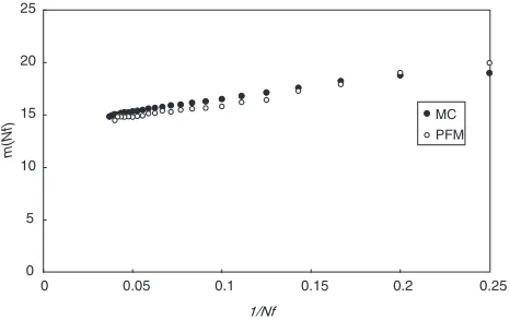
Figure 16 shows comparison ofmðNfÞversusNf relation obtained by the phase field model and that by the Monte Carlo simulation. It is shown that relations by both simulations are quite similar.
We find that topological results obtained by the phase field model are in good agreement with those by the Monte Carlo method. However it should be noted that the grain size and grain face distributions are affected by theJ=kTvalue. Effect of theJ=kT value on topology of grain structure is left as a future work.
0 20 40 60 80 100 120 140
0 1000 2000 3000 4000 5000
Time, MCS
[image:5.595.312.543.73.198.2]Area
Fig. 10 Average area versus time simulated by the Monte Carlo method.
0 0.2 0.4 0.6 0.8 1 1.2 1.4 1.6
0 0.5 1 1.5 2 2.5
R/Rav
400 MCS 500 MCS
750 MCS
1000 MCS
F
[image:5.595.51.287.234.365.2]requency
Fig. 11 Variation in the scaled grain size distribution function with time by the Monte Carlo method.
0 1 2 3 4 5 6 7 8 9 10
0 10 20 30 40
Number of faces per grain, Nf
400 MCS
500 MCS 750 MCS
1000 MCS
F
requency
, %
Fig. 12 Variation in the face number distribution function with time by the Monte Carlo method.
0 5 10 15 20 25
0 0.05 0.1 0.15 0.2 0.25
1/Nf
m(Nf)
Fig. 13 Relation between the average number of faces of neighbor of N-face grain,mðNfÞand the face number,Nf by the Monte Carlo method.
0 0.2 0.4 0.6 0.8 1 1.2 1.4
0 0.5 1 1.5 2 2.5
Rv/<Rv>
MCM
PFM
Hillert-3D
[image:5.595.310.544.253.388.2]f(Rv/<Rv>)
[image:5.595.55.285.417.554.2]3.4 Interrelation of the phase field and the Monte Carlo models
In previous section we found that grain size and grain face distributions given by phase field model were in good agreement with those by Monte Carlo method, So we try to interrelate a master equation of Monte Carlo method to a continuum model.
In the Monte Carlo algorithm a sequence of successive configurations are generated with help of (pseudo) random numbers and a suitably chosen transition probability. An efficient sampling technique to sample configurations from phase space was given by Metroplis.28) In the Metropolis algorithm the successive configurations are not chosen independently but rather via a Markov chain. A possibility is to use a Markov process which generates a configuration
fs0g from the knowledge of a configuration fsg. Let
Wðfsg;fs0gÞ be the conditional probability to select fs0g
stating from fsg, thus defining the Markov process. The successive states are generated with a particular transition probabilityWðfsg;fs0gÞ, which is chosen so that in the limit of
a large number of configurations the probabilityPðfsgÞtends toward the equilibrium distribution:
Peq¼exp½EðfsgÞ=kBT=Z; ð12Þ
whereE is an internal energy function,kBis the Boltzmann
constant,T is the temperature andZ is a canonical partition function. A sufficient condition to ensure this is the principle of detailed balance:
PeqðfsgÞWjðfsg;fs0gÞ ¼Peqðfs0gÞWjðfs0g;fsgÞ: ð13Þ The Monte Carlo algorithm may be interpreted via a master equation as describing a dynamical model with stochastic process.29)It satisfies the Markovian master equation as:
@Pðfsg;tÞ
@t ¼
X
fs0g
Pðfs0g;tÞWðfs0g;fsgÞ
X
fsg
Pðfsg;tÞWðfsg;fs0gÞ:
ð14Þ
The master equation is reduced to a differential equation of the Fokker–Planck type.30)It will be helpful conceptually to divide the alloy into microregions, each containing sites. We define the average values. We can choose the transition mechanism so that a particularschanges byþ(the order parameter s is non-conserved). This transition mechanism can be expressed mathematically by writingW in the form:
Wðfsg;fs0gÞ ¼X
Y
6¼ ðs0
sÞ
Z1
1
Rðfs0g;fsgÞðs0sÞd:
ð15Þ
The sum over assures that the thermal mechanism acts uniformly on all the sites in the system. The transition rate Rðfsg;fs0gÞcan be written as
Rðfs0g;fsgÞ ¼exp Ffs
0g Ffsg
2kBT
ðfs0g;fsgÞ; ð16Þ
whereðfsg;fs0gÞis a symmetric function in the initial and the final state,fsgandfs0g, andFfsgis a coarse-grained free
energy given by
Ffsg ¼Efsg kBTlnWfsg; ð17Þ
whereWfsgis the number of configuration consistent with a specific choice of average variable s. Note that the introduction of the factor Wfsg for computation of the transition rate required by the use of average variabless, has justified replacing the energies by free energies in eq. (17). Because of the restricted class of transitions (fsg to fs0g)
which is permitted by the form eq. (16),is a function only of, change ins. Since the coarse-grain cell contains a large number of sites, the change in scorresponding to a single transition is small. ThusðÞmust be sharply peaked around ¼0. For convenience, we introduce the jump rate, , though
Z1
1
2ðÞd1; ð18Þ
whereis the number of sites in the cell. Thusis the only adjustable phenomenological parameter. By defining the probability current vector by
J¼
2
1
kBT
@F
@s
Pþ @P
@s
; ð19Þ
we can rewrite the master equation in the form of the Fokker– Planck equation as
@Pfsg
@t ¼ X
@J @s
: ð20Þ
0 1 2 3 4 5 6 7 8 9 10
0 10 20 30 40
Number of faces per grain
MCM
PFM
F
requency
[image:6.595.52.285.74.209.2], %
Fig. 15 Comparison of the face number distribution function simulated by the phase field model with that by the Monte Carlo method.
0 5 10 15 20 25
0 0.05 0.1 0.15 0.2 0.25
1/Nf
PFM MC
m(Nf)
[image:6.595.53.286.255.402.2]In a continuum representation where rr~ is the position corresponding to site the summation on the cells become integral over the space according to
X
. . .¼ 1
ad Z
d~rr. . .: ð21Þ
It will be also convenient to introduce the functional derivative notation
@ @s
¼ad
sðrr~Þ; ð22Þ
wheredis the dimensionality of the model and a is the lattice constant. A Langevin type equation is simply the first moment of eq. (20). To see this we multiply eq. (20) bys and integrate over all thes’s. The result is
@ss @t ¼
Z s @P
@t
s¼
Z
Jfsgs
¼
2kBT
Z
s @F @s
P:
ð23Þ
In the continuum representation, eq. (23) becomes
@ss @t ¼
ad
2kBT
@F @s
; ð24Þ
where angular brackets denote the statistical average. Let us suppose that P is a sharply peaked function of thesin the neighborhood offsg ¼ fssg, so that average with respect toP of any function of fsg is well approximated by the same function offssg. Then eq. (24) becomes
@ss
@t ¼
ad
2kBT
FF
ss
: ð25Þ
Thus we obtain the time-dependent Gizburg–Landau equation for nonconserved order parameter from the master equation of the Monte Carlo method.
4. Summary
Temporal evolution and morphology of grain structure in three dimensions were simulated by the phase field and the Monte Carlo simulations. In order to prevent impingement of grain of like orientation, a new algorithm was adopted for both simulations.
The following results are obtained.
(1) Excluding the initial stage, the average area is found to be proportional to time in the phase field and the Monte Carlo simulations. The scaled grain size and the face number distributions become time-independent in both simulations.
(2) The scaled grain size and the face number distributions obtained by the phase field simulation are in good agreement with those by the Monte Carlo method. The nearest neighbor face correlation similar to the Aboav– Weaire relation is observed in simulated grain struc-tures by both methods. The nearest neighbor face correlation for the phase field model is quite similar to that for the Monte Carlo method.
(3) Interrelation between the phase field model and the Monte Carlo method is discussed.
REFERENCES
1) H. V. Atkinson: Acta Metall.36(1988) 469–401.
2) D. Weaire and J. A. Glazier: Mater. Sci. Forum94–96(1992) 27–38. 3) M. Hillert: Acta Metall.13(1965) 227–238.
4) J. E. Burke and D. Turnbull: Prog. Met. Phys.3(1952) 220–292. 5) N. P. Louat: Acta Metall.22(1974) 721–724.
6) D. Weaire and F. Bolton: Phys. Rev. Lett.65(1990) 3449–3451. 7) D. Weaire and J. P. Kermode: Philos. Mag. B48(1983) 245–249. 8) D. Weaire and H. Lei: Philos. Mag. Lett.62(1990) 427–430. 9) K. Kawasaki, T. Nagai and K. Nakashima: Philos. Mag. B60(1989)
399–421.
10) C. V. Thompson, H. J. Frost and F. Spaepen: Acta Metall.35(1987) 887–890.
11) M. P. Anderson, D. J. Srolovitz, G. S. Grest and P. S. Sahni: Acta Metall.32(1984) 783–791.
12) D. J. Srolovitz, M. P. Anderson, P. S. Sahni and G. S. Grest: Acta Metall.32(1984) 793–802.
13) D. Fan and L. Q. Chen: Acta Mater.45(1997) 611–632.
14) D. Fan, C. Geng and L. Q. Chen: Acta Metall.45(1997) 1115–1126. 15) J. Wejchert, D. Weaire and J. P. Kermode: Philos. Mag. B53(1986)
15–24.
16) M. P. Anderson, G. S. Grest and D. J. Srolovitz: Philos. Mag. B59
(1989) 293–329.
17) J. D. Srolovitz, G. S. Grest and M. P. Anderson: Acta Metall.33(1985) 2233–2247.
18) J. D. Srolovitz, G. S. Grest, M. P. Anderson and A. D. Rollet: Acta Metall.36(1985) 2115–2128.
19) V. Tikare, E. A. Holm, D. Fan and l. Q. Chen: Acta Mater.47(1999) 363–371.
20) V. Tikare and E. A. Holm: J. Am. Ceram. Soc.81(1998) 480–484. 21) S. R. de Groot and P. Mazur: Non-Equilibrium Thermodynamics,
(Dover, New York, 1984).
22) Y. Saito: ISIJ Int.38(1998) 559–566.
23) C. E. Krill and l. Q. Chen: Acta Mater.50(2002) 3057–3073. 24) J. W. Cahn and J. E. Hilliard: J. Chem. Phys.28(1958) 258–267. 25) S. M. Allen and J. W. Cahn: Acta Metall.27(1979) 1085–1095. 26) D. A. Aboav: Metallography5(1970) 251–263.
27) D. Weaire and N. Rivier: Contemporary Physics25(1984) 59–99. 28) K. Binder ed.:Monte Carlo Methods in Statistical Physics, 2nd ed.,
(Springer Verlag, Berlin, 1986).
29) D. W. Heermann: Computer Simulation Methods in Theoretical Physics, (Springer Verlag, Berlin, 1986).