Quantitative Evaluation of Interdiffusion in Fe2Al5 during Reactive Diffusion in the Binary Fe–Al System

Quantitative Evaluation of Interdiffusion in Fe

Al

during Reactive Diffusion

in the Binary Fe–Al System

Masanori Kajihara

Department of Materials Science and Engineering, Tokyo Institute of Technology, Yokohama 226-8502, Japan

Using Al/Fe/Al diffusion couples prepared by a diffusion bonding technique, the reactive diffusion in the binary Fe–Al system was experimentally examined in a previous study. The diffusion couple was isothermally annealed at temperatures ofT¼823{913K, and then a compound layer of Fe2Al5was observed to form at the interface. The observation indicates that there exists the parabolic relationship between the mean thickness of the Fe2Al5layer and the annealing time. The parabolic relationship means that the growth of the Fe2Al5layer is controlled by volume diffusion. A mathematical model for the reactive diffusion controlled by volume diffusion was used in order to analyze numerically the growth rate of the Fe2Al5 layer. Through the analysis, the interdiffusion coefficientDof Fe2Al5 was evaluated to be 5:931016, 1:181014 _{and 2:9210}14_m2_{/s at T¼823, 873 and 913 K, respectively. Expressing the temperature dependence of D as D¼}

D0expðQ=RTÞ, values ofD0¼2:34102m2/s andQ¼276kJ/mol were obtained by the least-squares method. [doi:10.2320/matertrans.47.1480]

(Received March 6, 2006; Accepted April 6, 2006; Published June 15, 2006)

Keywords: intermetallic compounds, bulk diffusion, analytical methods, reactive diffusion, kinetics

1. Introduction

In many binary alloy systems, intermetallic compounds

appear as stable phases.1) When a diffusion couple is

prepared from two different pure metals in such a binary system and then annealed at an appropriate solid-state

temperature T, some of the compounds may be discerned

to form as layers at the interface between the two metals after certain periods due to reactive diffusion. Many investigators experimentally studied the reactive diffusion in various alloy systems.2–24)_{If the reactive diffusion is governed by volume}

diffusion, the total thickness l of the compound layers is

expressed as a function of the annealing time t by the

parabolic relationship l2_{¼Kt. Here, K is the parabolic}

coefficient. The parabolic relationship may be usually believed to hold good in many binary systems. However, the volume diffusion is not necessarily the rate-controlling process of reactive diffusion for all the binary systems.11–23)

The reactive diffusion in the binary Au–Sn system was experimentally observed using Sn/Au/Sn diffusion couples prepared by a diffusion bonding technique in previous studies.15–17)The diffusion couple was isothermally annealed

at temperatures betweenT¼393and 473 K. During

anneal-ing, compound layers consisting of AuSn, AuSn2and AuSn4

are produced at the Au/Sn interface in the diffusion couple. The total thickness of the compound layers is proportional to a power function of the annealing time, and the exponent of the power function is 0.48, 0.42 and 0.36 atT¼393, 433 and 473 K, respectively. Thus, the parabolic relationship does not hold good for the binary Au–Sn system. The temperature dependence of the exponent implies that grain boundary diffusion contributes to the rate-controlling process of reactive diffusion and grain growth takes place in the compound layers at certain rates at higher annealing temper-atures. As the annealing temperature decreases, the contri-bution of grain boundary diffusion becomes remarkable, but

the grain growth slows down. Such temperature dependence of the rate-controlling process was reported also for the

binary Ag–Sn and Ni–Sn systems.18,19)

As to the binary Ni–Sn system, the reactive diffusion was experimentally observed using Sn/Ni/Sn diffusion couples

prepared by the diffusion bonding technique.19) In that

experiment, the diffusion couple was isothermally annealed atT ¼433{473K, and then a compound layer of Ni3Sn4was

discerned at T ¼453{473K along the interface in the

diffusion couple. The mean thickness of the Ni3Sn4 layer is

expressed as a power function of the annealing time, and the exponent of the power function takes values of 0.46 and 0.41

atT ¼453and 473 K, respectively. The exponent is smaller

than 0.5 at higher annealing temperatures, and approaches to 0.5 at lower annealing temperatures. Therefore, the same temperature dependence of the rate-controlling process as the binary Au–Sn system works also for the binary Ni–Sn system.

The reactive diffusion was experimentally observed for the

binary Fe–Al system in a previous study.25)The experiment

was carried out using Al/Fe/Al diffusion couples prepared by the diffusion bonding technique. Owing to annealing at

T ¼823{913K, a compound layer of Fe2Al5is formed at the

interface in the diffusion couple, and grows according to the parabolic relationship. This means that the growth of the Fe2Al5 layer is controlled by volume diffusion. This type of

rate-controlling process was observed also for the binary Pd–Sn system.22)_{In this system, compound layers consisting}

of PdSn4, PdSn3 and PdSn2 are formed at T¼433K, but

those composed of only PdSn4 and PdSn3 are produced at

T ¼453and 473 K. At all these temperatures, however, there exists the parabolic relationship between the total thickness of the Pd–Sn compound layers and the annealing time. Consequently, the rate-controlling process of reactive dif-fusion varies depending on the alloy system.

The kinetics of the reactive diffusion controlled by volume diffusion was theoretically analyzed using a mathematical model in a previous study.26) In the theoretical analysis, a *_{Corresponding author, E-mail: [email protected]}

hypothetical binary alloy system consisting of two primary solid solution phases and one intermetallic compound was considered in order to evaluate the growth rate of the compound in various semi-infinite diffusion couples initially composed of the two primary solid solution phases with different solubility ranges and interdiffusion coefficients. The mathematical model was also used to analyze numerically the relationship between the temperature dependence of the interdiffusion in each phase and the kinetics of the reactive

diffusion.27–29) _{As mentioned earlier, a single compound}

layer is formed during reactive diffusion in the binary Ni–Sn and Fe–Al systems.19,25)The growth of the compound layer is controlled by volume diffusion for the binary Fe–Al system, but by volume diffusion and grain boundary diffusion for the binary Ni–Sn system. As a consequence, the mathematical model26)can be used to describe the growth behavior of the compound layer for the former binary system. In the present study, the experimental results of the reactive diffusion in the

binary Fe–Al system25) _{have been numerically analyzed}

using the mathematical model. The interdiffusion coefficient in the compound layer has been evaluated through the analysis.

2. Experimental Summary

As mentioned earlier, the reactive diffusion in the binary Fe–Al system was experimentally observed in a previous study.25)In that experiment, Al/Fe/Al diffusion couples were prepared by a diffusion bonding technique, and then isothermally annealed at solid-state temperatures between

T ¼823and 913 K. During annealing, a compound layer of

Fe2Al5 is produced at the interface in the diffusion couple.

According to a recent phase diagram in the binary Fe–Al system,30)_{FeAl, FeAl}

2 and FeAl3 as well as Fe2Al5 should

appear as stable compounds atT ¼823{913K. Of these four

compounds, however, only Fe2Al5was recognized under the

present experimental conditions. This indicates that the

formation rate is much smaller for FeAl, FeAl2 and FeAl3

than for Fe2Al5. The compounds with low formation rates

cannot grow to visible thicknesses within experimental annealing times. For the Fe2Al5 layer, the mean thicknessl

was experimentally determined at each annealing time. The values oflare plotted against the square root oftin Fig. 1. In this figure, open triangles, squares and circles show the

results of T¼823, 873 and 913 K, respectively. Although

the open circle at t¼2:16104_{s and the open square at}

t¼4:32104_{s are slightly scattered in Fig. 1, most of}

the plotted points are located well on the corresponding straight line. This means that the parabolic relationship holds

good between the thickness l and the annealing time t as

follows.

l2¼Kt ð1Þ

Here,Kis the parabolic coefficient with a dimension of m2_/s.

From the plotted points in Fig. 1, the value of K was

evaluated at each temperature by the least-squares method. The evaluation gives K¼1:601016_{, 3:4110}15 _and 8:461015m2/s forT¼823, 873 and 913 K, respectively. Using these values ofK,lwas calculated as a function oft

from eq. (1). The results of T¼823, 873 and 913 K are

indicated as dotted, dashed and solid lines, respectively, in Fig. 1.

The values of Kare plotted against the temperature T as

open squares in Fig. 2. In this figure, the ordinate shows the logarithm ofK, and the abscissa indicates the reciprocal ofT.

If the temperature dependence of K is expressed by the

equation

K¼K0expðQK=RTÞ; ð2Þ

the pre-exponential factorK0and the activation enthalpyQK are evaluated to be1:32102m2/s and 281 kJ/mol, respec-tively, from the open squares in Fig. 2 by the least-squares method. Here,Ris the gas constant. Using these parameters,

Kwas calculated as a function ofTfrom eq. (2). The result is shown as a dashed line in Fig. 2.

Fig. 1 The mean thicknesslof the Fe2Al5layer versus the square root of the annealing time t shown as open triangles, squares and circles at

T¼823, 873 and 913 K, respectively. Straight lines indicate the calculations from eq. (1).

Fig. 2 The parabolic coefficientKof the Fe2Al5layer versus the reciprocal of the annealing temperatureTshown as open squares. The evaluations for the interdiffusion coefficientD_{of Fe}

3. Model

In order to analyze theoretically the kinetics of the reactive diffusion controlled by volume diffusion, a hypothetical binary A–B system consisting of one intermetallic compound and two primary solid solution phases was adopted in previous studies.26–29)Theandphases are the primary solid solution

phases of elements A and B, respectively, and thephase is

the compound. Now, we consider a semi-infinite diffusion

couple composed of the and phases with initial

compositions ofy0_andy0_{, respectively. Here,yis the mol}

fraction of element B. In the semi-infinite diffusion couple, the

thickness is semi-infinite for theandphases, and the=

interface is flat. Therefore, the interdiffusion of elements A and B occurs unidirectionally along the direction perpendic-ular to the flat interface. This direction is called the diffusional direction. If the diffusion couple is annealed at temperatureT

for an appropriate time, thephase will be formed as a layer

along the interface owing to reactive diffusion between the

and phases. The concentration profile of element B across

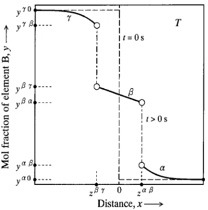
thephase layer along the diffusional direction is schemati-cally drawn in Fig. 3.26)In this figure, the ordinate shows the

mol fraction y, and the abscissa indicates the distance x

measured from the initial position of the = interface.

Dashed lines and solid curves show the concentration profiles

before and after annealing, respectively, and z _{and z}

indicate the positions of the = and = interfaces,

respectively, after annealing. When the local equilibrium is realized at each migrating interface during annealing, the compositions of the neighboring phases at the interface coincide with those of the corresponding phase boundaries at temperatureTin the phase diagram of the binary A–B system. Consequently, the migration of the interface is controlled by the volume diffusion in the neighboring phases. In Fig. 3,y

and y are the compositions of the and phases,

respectively, at the=interface, andy andyare those

of theandphases, respectively, at the=interface. The

compositions y, y, y and y give the boundary

conditions, and thosey0_andy0_{provide the initial conditions.}

For the reactive diffusion governed by volume diffusion,

the positionsz _{andz of the= and= interfaces are}

described as functions of the annealing time t by the

equations

z¼Kp4ffiffiffiffiffiffiffiffiffiffiD_t¼Kpffiffiffiffiffiffiffiffiffiffi_{4Dt ð3aÞ} and

z ¼Kpffiffiffiffiffiffiffiffiffiffi4D_t¼Kpffiffiffiffiffiffiffiffiffiffi_{4Dt; ð3bÞ}

respectively.31)_{Here, D, D and D are the interdiffusion}

coefficients for volume diffusion in the , and phases,

respectively, and K,K,K andKare dimensionless

coefficients. The thickness l of the phase layer is

determined as the difference between z andz, and thus

the following equation is obtained from eq. (3) to expresslas a function oft.

l2¼ ðzzÞ2¼4DðKKÞ2t¼Kt ð4Þ

Equation (4) again indicates the parabolic relationship.

According to eq. (4), K is described as a function of D_,

K_{andK by the following equation.}

K 4DðKKÞ2 ð5Þ

The dimensionless coefficients are related to the initial and boundary conditions as follows:

cc¼ c 0_c

Kpffiffiffi_f1erfðKÞgexpfðK _Þ2_g

þ c

_c

Kpffiffiffi_{ferfðKÞ erfðKÞg}expfðK

Þ2g ð6aÞ

and

cc ¼ c

_c

Kpffiffiffi_{ferfðKÞ erfðKÞg}expfðK

Þ2g

þ c 0_c

Kpffiffiffi_{f1þerfðKÞg}expfðK

_Þ2_{g: ð6bÞ}

Here,cis the concentration of element B measured in mol per unit volume. The initial and boundary conditions are indicated with the concentrationcin eq. (6), but shown with the mol fractionyin Fig. 3. However,yis readily converted

into c by the equation c¼y=Vm, where Vm is the molar

volume of the relevant phase. The following relationships are deduced from eq. (3):

K¼KpffiffiffiffiffiffiffiffiffiffiffiffiffiffiD_{=D ð7aÞ}

and

K¼KpffiffiffiffiffiffiffiffiffiffiffiffiffiffiD_{=D: ð7bÞ}

Equation (7) indicates that only two of the four

dimension-less coefficients are independent. In the present study, K

andK_{are chosen as the independent variables. Insertion of}

eq. (7) into eq. (6) yields two independent equations. As a result, the two independent variables are finally determined from the two independent equations.

4. Results and Discussion

As mentioned in Section 3, the mol fraction y is readily

converted into the concentrationcby the equationc¼y=Vm.

Here, Vm is the molar volume of the relevant phase. The

molar volumesVAl

m andV Fe

m of Al and Fe are10:010

6_and

7:10106_m3_{/mol, respectively, at room temperature.}32)

Thus,VAl

m is 40 percent greater thanVmFe. On the other hand,

the diffusion coefficientD_{of thephase is expressed as a}

function of the temperatureT by the following equation of

the same formula as eq. (2).

D¼D₀expðQ=RTÞ ð8Þ

Here, D

0 is the pre-exponential factor, and Q

_{is the}

activation enthalpy. Hereafter, the Fe, Fe2Al5 and Al phases

are denoted by ¼, and , respectively. Values of

D

0 ¼5:210

4_m2_{/s and Q¼246kJ/mol are reported}

for D _{of the phase with the body-centered cubic (bcc)}

structure, and those ofD₀ ¼1:2105_m2_{/s andQ ¼135}

kJ/mol are obtained for D _{of the phase with the}

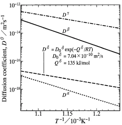
face-centered cubic (fcc) structure.32)_{Using these parameters,D}

was calculated as a function ofTfrom eq. (8). The results of

DandD are shown as dotted and dashed-and-dotted lines,

respectively, in Fig. 4. As can be seen,Dis more than four

orders of magnitude greater thanD. Although the diffusion

coefficients and the molar volumes of the constituent phases

affect the value of K through eqs. (5)–(7), the difference

between the molar volumes is negligible compared with that between the diffusion coefficients. Thus, we may assume with sufficient accuracy that the molar volume is equivalent

among the,andphases. On the basis of this assumption,

the concentrationcin eq. (6) is automatically replaced with the mol fractiony.

According to a phase diagram in the binary Fe–Al

system,30) _{the solubility of Fe in the phase is about}

0.2 at% atT¼823{913K. Thus,y_{is considered to take a}

constant value of 0.998 atT ¼823{913K. Here,yindicates

the mol fraction of Al. The phase possesses a constant

solubility range between y¼0:70andy ¼0:73at T¼

823{913K. On the other hand, the solubilityyof Al in the

phase is 0.222, 0.227 and 0.232 atT¼823, 873 and 913 K, respectively. The temperature dependence of solubility may be described by an equation of the same formula as eqs. (2)

and (8). As to the phase in the binary Fe–Al system,

however, this type of equation cannot reproduce accurately

the value of y _{at each temperature. In contrast, the}

following equation is suitable for expression of the

temper-ature dependence ofy_{atT ¼823{913K.}

y¼a0þa1Tþa2T2 ð9Þ

For the valuesy_{¼0:222, 0.227 and 0.232 atT ¼823, 873}

and 913 K, respectively, a0, a1 and a2 in eq. (9) are

determined to be 3:57101_{, 4:1110}4 _{and 3:00}

107_{, respectively. Furthermore,y}0_¼0andy0_{¼1for the}

Al/Fe/Al diffusion couple. Under such initial and boundary

conditions,Dwas evaluated from eqs. (5)–(7) usingDand

Din Fig. 4 in order to reproduce the experimental values of

Kin Fig. 1. The evaluation givesD¼5:931016,1:18 1014 and 2:921014m2/s at T ¼823, 873 and 913 K, respectively. These values ofDare shown as open circles in Fig. 2. If the relationship betweenD_{andK is described by}

the equation

D¼fK; ð10Þ

the following equation is readily obtained from eqs. (5) and (10).

f ¼0:25ðKKÞ2 ð11Þ

In order to estimateD_{fromK,f may be sometimes assumed}

as 1, 0.5 or 0.25 in eq. (10). This assumption insists thatDis not greater thanK. However, the value of f calculated from eq. (11) is greater than unity.26)Actually, f is equal to 3.69,

3.45 and 3.45 atT ¼823, 873 and 913 K, respectively, and

thus D is greater than K. This means that the values f ¼

10:25 yield underestimation of D_{. If the temperature}

dependence of D _{is described by eq. (8), D}

0 and Q _are

evaluated to be2:34102_m2_{/s and 276 kJ/mol,}

respective-ly, from the open circles in Fig. 2 by the least-squares

method. Using these parameters, D _{was calculated as a}

function ofT from eq. (8). The result is indicated as a solid line in Fig. 2. SinceQ_{is close toQ}

K, the solid line is almost parallel to the dashed line. The solid line in Fig. 2 is represented also as a solid line in Fig. 4. As can be seen,D_is

smaller thanD_{, but much greater thanD.}

In the experiment mentioned in Section 2, the Al/Fe/Al

diffusion couple was annealed atT ¼823, 873 and 913 K up

to t¼4:32105,1:73105 and2:59105s, respective-ly.25)Under such experimental conditions, the FeAl, FeAl2,

Fe2Al5 and FeAl3 phases are expected to form in the

diffusion couple.30) _{However, only the Fe}

2Al5 layer was

observed even at the longest annealing time for each temperature. The spatial resolution of electron probe

micro-analysis (EPMA) is around 1mm. Hence, the compound layer

with a thickness smaller than 1mm is invisible in the

concentration profile determined by EPMA. For convenience sake, such an invisible Fe–Al compound is called thephase. Inserting t¼4:32105_{, 1:7310}5 _{and 2:5910}5_{s with}

l¼1106_{m into eq. (1), we obtain K¼2:3110}18_,

5:791018 _{and 3:8610}18_m2_{/s for T ¼823, 873 and}

913 K, respectively. These values correspond to the upper

limits of K for the phase. Combining K¼2:311018_,

5:791018and3:861018m2/s withf ¼3:69, 3.45 and 3.45, we gainD ¼8:551018,2:001017 and1:33 1017_m2_{/s forT ¼823, 873 and 913 K, respectively, from}

Fig. 4 The interdiffusion coefficient D _{versus the reciprocal of the}

annealing temperatureTshown as various straight lines for the,,and

eq. (10). These values also correspond to the upper limits of

D_{. Since the melting temperature is higher for the phase}

than for the phase,30) _{volume diffusion will occur more}

sluggishly in the phase than in the phase at solid-state

temperatures. This implies thatQ_{cannot be smaller thanQ.}

In order to estimate the consistent upper limit ofD_{, values of}

D

0¼7:041010m2/s and Q ¼135kJ/mol are finally

obtained atT ¼823{913K. Using these parameters,D _was

calculated as a function ofTfrom eq. (8). The result is shown as a dashed line in Fig. 4. As can be seen,D_{is much smaller}

than D and D, but slightly greater than D. It is worth

repeating thatDindicates the upper limit. Consequently, for

¼FeAl, FeAl2and FeAl3,Dshould be smaller thanDat

T ¼823{913K.

5. Conclusions

The reactive diffusion in the binary Fe–Al system was

experimentally observed in a previous study.25) _{In that}

experiment, Al/Fe/Al diffusion couples were prepared by the diffusion bonding technique, and then isothermally

annealed at temperatures between T¼823 and 913 K.

During annealing, a compound layer of Fe2Al5is formed at

the interface in the diffusion couple, and grows according to

the parabolic relationship l2_{¼Kt, where l is the mean}

thickness of the Fe2Al5layer,tis the annealing time, andKis

the parabolic coefficient. This means that the growth of the Fe2Al5 layer is controlled by volume diffusion. The

obser-vation providesK¼1:601016,3:411015and8:46 1015m2/s atT ¼823, 873 and 913 K, respectively. In order

to evaluate the interdiffusion coefficient D of the Fe2Al5

phase, the experimental results were numerically analyzed using the mathematical model reported in a previous study.26)

The analysis yields D¼5:931016_{, 1:1810}14 _and

2:921014_m2_{/s atT ¼823, 873 and 913 K, respectively.}

If the temperature dependence of D is described by the

equation D¼D0expðQ=RTÞ, values of D0¼2:34

102_m2_{/s and Q¼276kJ/mol are obtained by the}

least-squares method. The interdiffusion coefficient of the Fe2Al5

phase is smaller than that of the fcc-Al phase, but much greater than that of the bcc-Fe phase.

Acknowledgements

The present study was supported by a Grant-in-Aid for Scientific Research from the Ministry of Education, Culture, Sports, Science and Technology of Japan.

REFERENCES

1) T. B. Massalski, H. Okamoto, P. R. Subramanian and L. Kacprzak:

Binary Alloy Phase Diagrams(ASM International, Materials Park, OH, 1990) vol. 1–3.

2) B. Lustman and R. F. Mehl: Trans. Met. Soc. AIME147(1942) 369– 394.

3) D. Horstmann: Stahl Eisen73(1953) 659–665.

4) S. Storchheim, J. L. Zambrow and H. H. Hausner: Trans. Met. Soc. AIME200(1954) 269–274.

5) G. V. Kidson and G. D. Miller: J. Nucl. Mater.12(1964) 61–69. 6) K. Shibata, S. Morozumi and S. Koda: J. Japan Inst. Met.30(1966)

382–388.

7) K. Hirano and Y. Ipposhi: J. Japan Inst. Met.32(1968) 815–821. 8) M. M. P. Janssen: Metall. Trans.4(1973) 1623–1633.

9) G. F. Bastin and G. D. Rieck: Metall. Trans.5(1974) 1817–1826. 10) M. Onishi and H. Fujibuchi: Trans. JIM16(1975) 539–547. 11) EI-B. Hannech and C. R. Hall: Mater. Sci. Tech.8(1992) 817–824. 12) P. T. Vianco, P. F. Hlava and A. L. Kilgo: J. Electron. Mater.23(1994)

583–594.

13) M. Watanabe, Z. Horita and M. Nemoto: Interface Science4(1997) 229–241.

14) S. Choi, T. R. Bieler, J. P. Lucas and K. N. Subramanian: J. Electron. Mater.28(1999) 1209–1215.

15) M. Kajihara, T. Yamada, K. Miura, N. Kurokawa and K. Sakamoto: Netsushori43(2003) 297–298.

16) T. Yamada, K. Miura, M. Kajihara, N. Kurokawa and K. Sakamoto: J. Mater. Sci.39(2004) 2327–2334.

17) T. Yamada, K. Miura, M. Kajihara, N. Kurokawa and K. Sakamoto: Mater. Sci. Eng. A390(2005) 118–126.

18) K. Suzuki, S. Kano, M. Kajihara, N. Kurokawa and K. Sakamoto: Mater. Trans.46(2005) 969–973.

19) M. Mita, M. Kajihara, N. Kurokawa and K. Sakamoto: Mater. Sci. Eng. A403(2005) 269–275.

20) T. Takenaka, S. Kano, M. Kajihara, N. Kurokawa and K. Sakamoto: Mater. Sci. Eng. A396(2005) 115–123.

21) T. Takenaka, S. Kano, M. Kajihara, N. Kurokawa and K. Sakamoto: Mater. Trans.46(2005) 1825–1832.

22) T. Takenaka, M. Kajihara, N. Kurokawa and K. Sakamoto: Mater. Sci. Eng. A406(2005) 134–141.

23) M. Mita, K. Miura, T. Takenaka, M. Kajihara, N. Kurokawa and K. Sakamoto: Mater. Sci. Eng. B126(2006) 37–43.

24) T. Takenaka and M. Kajihara: Mater. Trans.47(2006) 822–828. 25) D. Naoi: Master Eng. Thesis, Tokyo Institute of Technology, 2006. 26) M. Kajihara: Acta Mater.52(2004) 1193–1200.

27) M. Kajihara: Mater. Sci. Eng. A403(2005) 234–240. 28) M. Kajihara: Mater. Trans.46(2005) 2142–2149.

29) M. Kajihara: Defect and Diffusion Forum249(2006) 91–95. 30) T. B. Massalski, H. Okamoto, P. R. Subramanian and L. Kacprzak:

Binary Alloy Phase Diagrams(ASM International, Materials Park, OH, 1990) vol. 1, p. 148.

31) W. Jost:Diffusion of Solids, Liquids, Gases (Academic Press, New York, 1960) p. 68.