Population growth and structural transformation

Munich Personal RePEc Archive

Population growth and structural

transformation

Ho, Chi Pui

The University of Hong Kong

19 November 2015

Online at

https://mpra.ub.uni-muenchen.de/73860/

Population Growth and Structural Transformation

*

HO, CHI PUI

The University of Hong Kong

4 September, 2016

ABSTRACT

This paper uncovers the mechanism and assumptions underlying how population growth induces structural transformation. We construct two-sector models that give analytically tractable closed-form solutions. If sectoral goods are consumption complements, population growth induces a more than proportionate relative price rise compared to the relative marginal product of labor drop in a sector with stronger diminishing returns to labor, and shifts production factors towards that sector.

Our work points to a two-stage development process: (1) in early development, population growth shifts production factors to agriculture; and (2) when agricultural productivity growth is fast enough, production factors move out of agriculture.

Keywords: Structural transformation; Population growth effect; Relative price effects; Relative marginal product effects

JEL Codes: E1, N1, O5

*

I wish to thank Yulei Luo, Joseph S.K. Wu, Stephen Y.W. Chiu, Chenggang Xu, Chi-Wa Yuen, Paul S.H. Lau, Fang Yang and L. Rachel Ngai for helpful discussions, as well as seminar participants at the University of Hong Kong 2015. Financial support from the Hong Kong PhD Fellowship Scheme (PF11-08043) and Sir Edward Youde Memorial Fellowships (for Postgraduate Research Students 2013/14) are gratefully acknowledged.

1

“[P]opulation increases, and the demand for corn raises its price relatively to other things—more capital is profitably employed on agriculture, and continues to flow towards it”. (David Ricardo 1821, 361)

1

INTRODUCTION

The concepts of population growth and structural transformation are vital to the study and practice of economic development. At least since Malthus (1826), who argued that population multiplies geometrically and food arithmetically to raise food prices and depress real wages, scholars have been exploring the links between population growth and economic development (Kuznets 1960; Boserup 1965; Simon 1977; Kremer 1993; Diamond 2005). Recently, Leukhina and Turnovsky (2016) brought forward the idea that population growth induces structural transformation.1 Their focus was on simulating the contribution of population growth to structural development in England. However, the mechanism by which population growth induces structural transformation was not adequately addressed in their paper. The central thesis of this paper is to further delineate this mechanism, by constructing two-sector models that give analytically tractable closed-form solutions of structural development.

Traditionally, economists have focused on structural transformation away from agriculture since industrialization in the Western world (Clark 1960, 510-520; Kuznets 1966, 106-107; Chenery and Syrquin 1975, 48-50). Seldom has attention been paid to the sectoral shift towards agriculture before the industrialization breakthrough (see the English and United States examples in sections 3 and 7), when income, technology and capital stock progressed slowly. Indeed, population growth was perhaps the most salient change in the Malthusian economies, that contributed to structural transformation in pre-industrial times.2

We construct two models to explain the two-stage development process implied above. Our models are simple enough to deliver closed-form solutions that track the mechanisms and crucial assumptions by which population growth, as well as technological progress and capital deepening, induces structural transformation.

The basic model (section 4) examines structural transformation in pre-industrial times. It is

1

Structural transformation refers to factor reallocation across different sectors in the economy. More broadly, Chenery (1988, 197) defined structural transformation as “changes in economic structure that typically accompany growth during a given period or within a particular set of countries”. He considered industrialization, agricultural transformation, migration and urbanization as examples of structural transformation.

2

The role of population growth on structural transformation is often overlooked. One exception is Johnston and Kilby (1975, 83-84), who stated that population growth determines the rate and direction of structural transformation. They defined the rate of structural transformation from agriculture to non-agriculture as 𝑅𝑅𝑅𝑅𝑅𝑅=𝐿𝐿𝑛𝑛

𝐿𝐿𝑡𝑡(𝐿𝐿𝑛𝑛 ′ _{− 𝐿𝐿}

𝑡𝑡

′_{), where 𝐿𝐿}

𝑛𝑛 is non-farm employment, 𝐿𝐿𝑡𝑡 is

total labor force, and 𝐿𝐿′_𝑛𝑛 and 𝐿𝐿′_𝑡𝑡 are their respective rates of change. They noted that, ceteris paribus,

“[t]he impact of a high rate of population growth (𝐿𝐿′_𝑡𝑡) is, of course, to diminish the value of

(𝐿𝐿′_𝑛𝑛− 𝐿𝐿′_𝑡𝑡). In Ceylon, Egypt, and Indonesia, high rates of population growth equalled or surpassed 𝐿𝐿′_𝑛𝑛 in recent decades so that structural transformation ceased or was reversed.”

2

a two-sector (agricultural and manufacturing), two-factor (labor and land) model.3 In the model, the representative household views agricultural and manufacturing goods as consumption complements, while agricultural production possesses stronger diminishing returns to labor. Holding sectoral factor shares constant, population growth will increase manufacturing output relative to agricultural output, raising the relative price of agricultural goods (relative price effect). At the same time, the increase in labor input in the two sectors will reduce the relative marginal product in the agricultural sector (relative marginal product effect). Given that the two sectoral goods are consumption complements, the relative price effect originating from the households’ unwillingness to consume too few agricultural goods relative to manufacturing goods will outride the relative marginal product effect. Since factor return equals output price times marginal product, this will relatively boost agricultural factor returns and draw production factors towards the agricultural sector. We call this the population growth effect on structural transformation.4 We will apply this model to simulate the rise (and fall) of agricultural labor share in pre-industrial England (AD1521-AD1745). Note that as the focus of this paper leans more towards the theoretical side, the simulations are more for illustrative purposes.

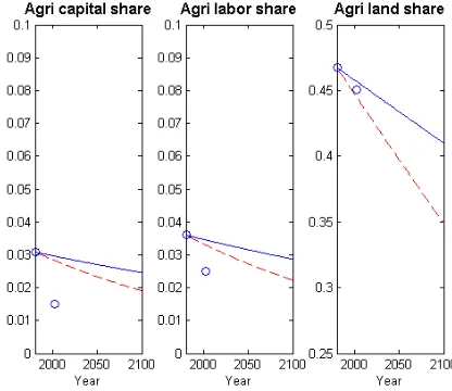
Next, the unified model (section 5) examines structural transformation in the modern times. Population is still an important component. We extend the basic model by allowing for technological progress and including capital as another production input. There are four relative price effects that foster structural transformation in the model, namely the agricultural technology growth effect, the manufacturing technology growth effect, the population growth effect and the capital deepening effect. From our analytical solution, to move production factors away from agriculture, we need a fast enough agricultural technology growth rate so that the agricultural technology growth effect overrides the other three relative price effects. We will apply this model to simulate the fall of agricultural factor shares in the modern United States (AD1980-AD2100). Part of the success of our work is the reconciliation of the fall in agricultural land share throughout development, which is not featured elsewhere in the structural transformation literature.

The next section reviews the relevant literature. Section 3 describes historical facts related to sectoral shifts in pre-industrial England and the modern United States. Section 4 develops the basic model. Section 5 extends it to the unified model. In section 6 we calibrate the two models to simulate sectoral shifts in pre-industrial England and the modern United States respectively. Section 7 highlights some discussion. Section 8 concludes.

2

RELATED LITERATURE

Our work is related to three bodies of literature. The first is the causes of structural transformation, which can be traced back to the work by Harris and Todaro (1970). They hypothesized that when the rural wage is lower than the expected urban wage, labor will migrate

3

In this paper, “manufacturing sector” refers to non-agricultural sector.

4

David Ricardo mentioned that population growth attracts capital towards the agricultural sector through the relative price effect. See his quote ahead of the Introduction.

3

from the rural to the urban sector. In their model labor movement is a disequilibrium phenomenon in the sense that unemployment exists. The literature has evolved to consider how structural transformation occurs within frameworks where full employment and allocation efficiency are achieved. Income effect and relative price effect originating from technology growth have become standard channels to explain structural transformation within these frameworks. The former is a demand-side approach, which assumes a non-homothetic household utility function, usually with a lower income elasticity on agricultural goods than on non-agricultural goods. Hence income growth throughout development process will shift demand away from the agricultural goods, fostering a relative agricultural decline in the economy. For example, Matsuyama (1992), Laitner (2000), Kongsamut et al. (2001), Gollin et al. (2002, 2007), Foellmi and Zweimüller (2008), Gollin and Rogerson (2014) shared this property. The latter is a supply-side approach, which emphasizes that differential productivity growth across sectors will bring along relative price changes among consumption goods. And the resulting direction of sectoral shift will depend on the degree of substitutability among different consumption goods. For example, Hansen and Prescott (2002), Doepke (2004), Ngai and Pissarides (2007, 2008), Acemoglu and Guerrieri (2008), Bar and Leukhina (2010) and Lagerlöf (2010) shared this feature. Acemoglu and Guerrieri (2008) proposed capital deepening as an additional cause that generates structural transformation through the relative price effect.

In the recent years, the literature has evolved to look into alternative explanations for structural transformation. For example, models with education/training costs (Caselli and Coleman 2001), tax changes (Rogerson 2008), barriers to labor reallocation and adoption of modern agricultural inputs (Restuccia et al. 2008), transportation improvement (Herrendorf et al. 2012), scale economies (Buera and Kaboski 2012a), human capital (Buera and Kaboski 2012b) and international trade (Uy et al. 2013) have been proposed. See Herrendorf et al. (2014) for a survey. Leukhina and Turnovsky (2016) posited population growth as another cause of structural transformation. They relied on simulating FOC conditions from a general equilibrium model to study structural development. In comparison, this paper will derive analytical closed-form solutions for sectoral share evolution, which shed light on the underlying mechanism and crucial assumptions of the population growth effect on structural transformation (sections 4.2 and 5.4).5

The second set of literature is related to developing unified models for structural transformation. Echevarria (1997), Acemoglu and Guerrieri (2008), Dennis and Iscan (2009), Duarte and Restuccia (2010), Alvarez-Cuadrado and Poschke (2011), and Guilló et al. (2011)’s works were in this direction. They constructed micro-founded models by blending at least two of the following causes of structural transformation: non-homothetic preference, biased technological progress and capital deepening. They either employed the models to simulate cross-sectional or time-evolving sectoral share patterns, or evaluated the relative importance of the above causes in accounting for historical structural changes. Hansen and Prescott (2002), Leukhina and Turnovsky (2016) also constructed unified models, where population growth is a cause of

5

Population growth is exogenous in this paper (sections 4 and 5). This allows us to focus on how population growth by itself gives rise to structural transformation. See Ho (2016) who incorporates the population growth effect on structural transformation in a framework with endogenous population growth to reconcile Eurasian economic history.

4

structural transformation. Again, as mentioned in the previous paragraph, they shared the methodology of relying on FOC simulations but not closed-form solutions to analyze structural development.

The third body of literature is related to the effect of population growth on per capita income evolution in growth models. In Solow (1956), Cass (1965) and Koopmans (1965)’s exogenous growth models, diminishing marginal product of capital assures saving in the economy just to replenish capital depreciation and population growth in the steady state. A change in population growth rate has just a level effect but no growth effect on per capita income evolution in the long run. In the AD1990s, Jones (1995), Kortum (1997) and Segerstrom (1998) proposed semi-endogenous growth models, which incorporate R&D and assume diminishing returns to R&D. In steady states, these models predict that per capita income (or real wage) growth rate increases linearly with population growth rate.6 To summarize, the above literature predicts a non-negative effect of population growth rate on per capita income growth rate in steady states. In contrast, in our growth models with land as a fixed production factor, faster population growth can adversely affect per capita income growth rate, even when the economies have attained their asymptotic growth paths (sections 4.3 and 5.5).

3

HISTORICAL EVIDENCE

This section documents historical evidence related to structural transformation between agricultural and manufacturing sectors in pre-industrial England (section 3.1) and the modern United States (section 3.2). Besides motivating our models in sections 4 and 5, these historical evidence will also be used for calibrations in section 6.

3.1

Structural Transformation in pre-industrial England

Sectoral shift occurred in pre-industrial England. Figure 1 depicts Clark (2010, 2013)’s estimates of agricultural labor share in England during AD1381-AD1755.7 Agricultural labor share gradually rose during the early Modern Period and decisively declined after the

6

In the early AD1990s, before the emergence of semi-endogenous growth models, Romer (1990), Grossman and Helpman (1991) and Aghion and Howitt (1992) built first-generation endogenous growth models. They predict that economies with larger population sizes (rather than population growth rates) would grow faster (population scale effect). The reasons are that those economies could employ more research scientists and there are larger markets for successful innovative firms to capture.

However, the empirical evidence did not support the population scale effect (Jones 1995). In the late AD1990s, Peretto (1998), Howitt (1999) and Young (1998) constructed Schumpeterian endogenous growth models. These models nullify the population scale effect by introducing endogenous product proliferation: as population increases, it attracts entry of new product varieties. This reduces effectiveness of productivity improvement as R&D resources are spread thinner across the expanding research frontier, and reward to product quality innovation is dissipated.

7

In this paper, the term “agricultural labor share” refers to the proportion of labor allocated to the agricultural sector, but not the fraction of national income labor captures. Similar interpretation holds for the terms “agricultural capital share”, “agricultural land share”, “manufacturing labor share”, “manufacturing capital share” and “manufacturing land share”.

5

mid-seventeenth century.8

INSERT FIGURE 1 HERE

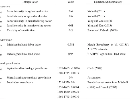
Structural transformation is commonly known to be caused by income growth (Kongsamut et al. 2001), biased technological progress (Ngai and Pissarides 2007) and capital deepening (Acemoglu and Guerrieri 2008). Before the Industrial Revolution, Britain was in its Malthusian era when income stagnation and slow capital accumulation characterized the country’s development. We also assume there was neglectable manufacturing technological progress in this period. Hence only agricultural productivity growth is left to explain sectoral shift. Table 1 shows Clark (2002)’s estimates of annual agricultural productivity growth rate in England during AD1525-AD1795. The magnitude of agricultural productivity growth during AD1525-AD1745 was quite moderate by modern standards.

INSERT TABLE 1 HERE

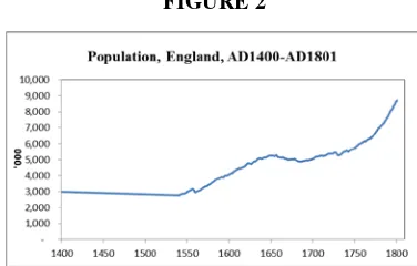
There is indeed another potential candidate which contributes to structural transformation: population growth. Figure 2 depicts Mitchell (1988) and Pamuk (2007)’s population estimates in England during AD1400-AD1801. Since AD1400, the English population had stayed at roughly 3 million for more than a century. It then rose at rates comparable to modern standards up till around AD1660. After that it stagnated at about 5 million until the eve of the Industrial Revolution.

INSERT FIGURE 2 HERE

We hypothesize that the interplay of population growth effect and agricultural technology growth effect on structural transformation explains agricultural labor share movement in pre-industrial England. In section 4 we will abstract technological progress and construct the basic model. This allows us to focus on the population growth effect on structural transformation. Agricultural productivity growth will be added in section 6.1 when we simulate sectoral shift in pre-industrial England.

3.2

Structural Transformation in the modern United States

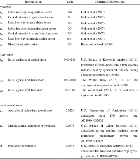
Sectoral shift has also occurred in the modern United States.9 Figure 3 depicts U.S. Bureau of Economic Analysis, or BEA (2016), and World Bank (2016)’s estimates of agricultural capital share (solid line), labor share (dashed line) and land share (dotted line) in the United States throughout AD1947-AD2013. All these factor shares were generally declining during their respective time frames.

INSERT FIGURE 3 HERE

We hypothesize that, in the modern times, agricultural and manufacturing technological

8

Broadberry et al. (2013) also provided estimates of agricultural labor share in England during AD1381-AD1861. Their estimates showed qualitatively the same rise-and-fall trend as Clark (2010, 2013)’s one, but the turning point occurred earlier, during the mid-sixteenth century. We will stay with Clark (2010, 2013)’s estimates throughout this paper.

9

For the United States, the term “agricultural sector” refers to the agricultural, forestry, fishing and hunting sectors defined by U.S. Bureau of Economic Analysis, or BEA (2016) in their NIPA Tables. The term “manufacturing sector” refers to all sectors other than agricultural, forestry, fishing and hunting.

6

progresses, population growth and capital deepening explain structural transformation. We examine the evolution of related variables in the United States during the late-twentieth and early-twenty-first centuries. Figure 4 depicts the farm total factor productivity in the United States during AD1948-AD2011, provided by U.S. Department of Agriculture (2016). Agricultural productivity was in general rising, and its growth had accelerated since the AD1980s.

INSERT FIGURE 4 HERE

Figure 5 depicts the annual multifactor productivity (SIC measures) for private nonfarm business sector in the United States during AD1948-AD2002, provided by U.S. Bureau of Labor Statistics, or BLS (2016). We use it to proxy manufacturing productivity. Manufacturing productivity was generally improving over time. It had suffered from a productivity growth slowdown since the AD1980s.

INSERT FIGURE 5 HERE

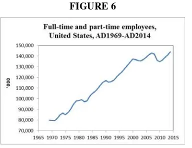
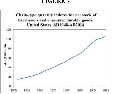
Figures 6 and 7 depict the number of full-time and part-time employees in the United States during AD1969-AD2013 and chain-type quantity indexes for net stock of fixed assets and consumer durable goods in the United States during AD1948-AD2013, provided by BEA (2016). Population growth and capital accumulation were both at work.

INSERT FIGURE 6 HERE INSERT FIGURE 7 HERE

In section 5 we will construct a unified model to account for structural transformation through the interplay of population growth effect, technology growth effects and capital deepening effect. In section 6.2 we will calibrate the unified model to simulate sectoral shift in the modern United States.

4

THE BASIC MODEL

4.1

Model setup (two-sector, two-factor)

We set up the basic model to examine the population growth effect on structural transformation. Households are homogenous. There are two sectors (agricultural and manufacturing) and two production factors (labor and land) in the economy. Markets are complete and competitive. Factors are mobile across the two sectors. Time is continuous and indexed by 𝑡𝑡.

The population at time 𝑡𝑡, 𝐿𝐿_𝑡𝑡, equals 𝐿𝐿₀ times 𝑒𝑒𝑛𝑛𝑡𝑡, where 𝐿𝐿₀ is the initial population and

𝑛𝑛 is the population growth rate. Each household is endowed with one unit of labor which is supplied inelastically. We assume households are altruistic towards their future generations. The representative household possesses lifetime utility function in the form of:

(1) ∫ 𝑒𝑒−(𝜌𝜌−𝑛𝑛)𝑡𝑡 𝑐𝑐̃𝑡𝑡1−𝜃𝜃−1

1−𝜃𝜃

∞

0 𝑑𝑑𝑡𝑡 ,

where 𝜌𝜌 is the discount rate, 𝜃𝜃 is the inverse of elasticity of intertemporal substitution, 𝑐𝑐̃_𝑡𝑡 is per capita consumption composite at time 𝑡𝑡.

The representative household makes consumption decisions {𝑐𝑐̃_𝑡𝑡}_𝑡𝑡=0∞ subject to budget

constraints at 𝑡𝑡 ∈[0,∞). At time 𝑡𝑡, the household owns one unit of labor and 𝑇𝑇

𝐿𝐿𝑡𝑡 unit of land. By supplying them to the market, the household obtains a wage income of 𝑊𝑊_𝑡𝑡(1) and a land rental income of 𝛺𝛺_𝑡𝑡𝑇𝑇

𝐿𝐿𝑡𝑡, where 𝑊𝑊𝑡𝑡 and 𝛺𝛺𝑡𝑡 are the nominal wage rate and land rental rate at time 𝑡𝑡.10 Formally, the budget constraint facing the representative household at time 𝑡𝑡 is:

(2) 𝑐𝑐̃_𝑡𝑡=𝑊𝑊𝑡𝑡

𝑃𝑃𝑡𝑡(1) +

𝛺𝛺𝑡𝑡

𝑃𝑃𝑡𝑡

𝑇𝑇 𝐿𝐿𝑡𝑡 ,

where 𝑃𝑃_𝑡𝑡 is the consumption composite price at time 𝑡𝑡.

Per capita consumption composite is a constant elasticity of substitution (CES) aggregator of per capita purchase of agricultural and manufacturing goods:

(3) 𝑐𝑐̃_𝑡𝑡=�𝜔𝜔_𝐴𝐴𝑦𝑦�_{𝐴𝐴𝑡𝑡}𝜀𝜀−1𝜀𝜀 +𝜔𝜔_𝑀𝑀𝑦𝑦�_{𝑀𝑀𝑡𝑡}𝜀𝜀−1𝜀𝜀 � 𝜀𝜀 𝜀𝜀−1

, 𝜔𝜔_𝐴𝐴,𝜔𝜔_𝑀𝑀∈(0,1), 𝜔𝜔_𝐴𝐴+𝜔𝜔_𝑀𝑀= 1, 𝜀𝜀𝜖𝜖[0,∞),

where 𝑦𝑦�_{𝐴𝐴𝑡𝑡}≡𝑌𝑌𝐴𝐴𝑡𝑡

𝐿𝐿𝑡𝑡 and 𝑦𝑦�𝑀𝑀𝑡𝑡≡

𝑌𝑌𝑀𝑀𝑡𝑡

𝐿𝐿𝑡𝑡 are per capita purchase of agricultural and manufacturing goods at time 𝑡𝑡 respectively, 𝜔𝜔_𝐴𝐴 and 𝜔𝜔_𝑀𝑀 are measures of relative strengths of demand for the two sectoral goods, 𝜀𝜀 is elasticity of substitution between the two sectoral goods. We denote the two sectoral goods to be consumption complements if 𝜀𝜀< 1, and to be consumption substitutes if

𝜀𝜀> 1.

Agricultural goods, 𝑌𝑌_{𝐴𝐴𝑡𝑡}, and manufacturing goods, 𝑌𝑌_{𝑀𝑀𝑡𝑡}, are produced competitively according to Cobb-Douglas technologies, using labor and land as inputs:

(4) 𝑌𝑌_{𝐴𝐴𝑡𝑡}=𝐴𝐴_𝑡𝑡𝐿𝐿𝛼𝛼_{𝐴𝐴𝑡𝑡}𝐴𝐴𝑅𝑅_{𝐴𝐴𝑡𝑡}𝛾𝛾𝐴𝐴, 𝛼𝛼_𝐴𝐴,𝛾𝛾_𝐴𝐴𝜖𝜖(0, 1), 𝛼𝛼_𝐴𝐴+𝛾𝛾_𝐴𝐴= 1, 𝑔𝑔_𝐴𝐴≡𝐴𝐴̇𝑡𝑡

𝐴𝐴𝑡𝑡= 0 ,

(5) 𝑌𝑌_{𝑀𝑀𝑡𝑡}=𝑀𝑀_𝑡𝑡𝐿𝐿𝛼𝛼_{𝑀𝑀𝑡𝑡}𝑀𝑀𝑅𝑅_{𝑀𝑀𝑡𝑡}𝛾𝛾𝑀𝑀, 𝛼𝛼_𝑀𝑀,𝛾𝛾_𝑀𝑀𝜖𝜖(0, 1), 𝛼𝛼_𝑀𝑀+𝛾𝛾_𝑀𝑀= 1, 𝑔𝑔_𝑀𝑀≡𝑀𝑀̇𝑡𝑡

𝑀𝑀𝑡𝑡= 0 ,

where 𝐿𝐿_{𝐴𝐴𝑡𝑡} and 𝐿𝐿_{𝑀𝑀𝑡𝑡}, 𝑅𝑅_{𝐴𝐴𝑡𝑡} and 𝑅𝑅_{𝑀𝑀𝑡𝑡} are labor and land employed by the two sectors at time 𝑡𝑡; 𝐴𝐴_𝑡𝑡 and 𝑀𝑀_𝑡𝑡 are agricultural and manufacturing productivities at time 𝑡𝑡; 𝛼𝛼_𝐴𝐴 and 𝛼𝛼_𝑀𝑀, 𝛾𝛾_𝐴𝐴 and 𝛾𝛾_𝑀𝑀 are labor intensities and land intensities in the two production sectors. In this section, to single out the population growth effect on structural transformation, we assume 𝐴𝐴_𝑡𝑡=𝐴𝐴 and 𝑀𝑀_𝑡𝑡=𝑀𝑀

for all 𝑡𝑡, that is, there are no technological progresses in the two sectors. Note that 𝛼𝛼_𝐴𝐴 and 𝛼𝛼_𝑀𝑀 measure the degree of diminishing returns to labor in the two sectors: the greater the values of these parameters are, the weaker diminishing returns to labor are.

Factor market clearing implies that the sum of factor demands from the two sectors equals aggregate factor supplies at each time 𝑡𝑡:

(6) 𝐿𝐿_{𝐴𝐴𝑡𝑡}+𝐿𝐿_{𝑀𝑀𝑡𝑡}=𝐿𝐿_𝑡𝑡 , (7) 𝑅𝑅_{𝐴𝐴𝑡𝑡}+𝑅𝑅_{𝑀𝑀𝑡𝑡}=𝑅𝑅 ,

where 𝑅𝑅 is the amount of land in the economy, which is fixed in supply for all time 𝑡𝑡.

10

To be more precise, the representative household also makes decision on whether to supply production factors to the agricultural or manufacturing sector. In equilibrium, factor returns in the two sectors will be equalized ((13) and (14)). Therefore we do not make a distinction between wages or land rentals in the two sectors in the representative household’s budget constraint (2).

8

Equations (1)-(7) describe our model economy. To proceed, we define 𝑌𝑌_𝑡𝑡 as the unique final output being produced competitively in the economy, using agricultural and manufacturing goods as intermediate inputs.

(8) 𝑌𝑌_𝑡𝑡=�𝜔𝜔_𝐴𝐴𝑌𝑌_{𝐴𝐴𝑡𝑡}𝜀𝜀−1𝜀𝜀 +𝜔𝜔_𝑀𝑀𝑌𝑌_{𝑀𝑀𝑡𝑡}𝜀𝜀−1𝜀𝜀 � 𝜀𝜀 𝜀𝜀−1

.

Technically, final output is an aggregator of agricultural and manufacturing output that represents the representative household’s consumption composite preference.11

We normalize the price of final output as the numéraire in the economy for all time 𝑡𝑡, that is:12

(9) 1≡(𝜔𝜔_𝐴𝐴𝜀𝜀𝑃𝑃_{𝐴𝐴𝑡𝑡}1−𝜀𝜀+𝜔𝜔_𝑀𝑀𝜀𝜀𝑃𝑃_{𝑀𝑀𝑡𝑡}1−𝜀𝜀)1−𝜀𝜀1 ,

where the associated prices of agricultural and manufacturing goods at time 𝑡𝑡, 𝑃𝑃_{𝐴𝐴𝑡𝑡} and 𝑃𝑃_{𝑀𝑀𝑡𝑡}, are respectively:

(10) 𝑃𝑃_{𝐴𝐴𝑡𝑡}=𝜔𝜔_𝐴𝐴�𝑌𝑌𝑡𝑡

𝑌𝑌𝐴𝐴𝑡𝑡� 1 𝜀𝜀

,

(11) 𝑃𝑃_{𝑀𝑀𝑡𝑡}=𝜔𝜔_𝑀𝑀� 𝑌𝑌𝑡𝑡

𝑌𝑌𝑀𝑀𝑡𝑡� 1 𝜀𝜀

.

Note that the consumption composite price always equals the final output price, that is, 𝑃𝑃_𝑡𝑡= 1

for all 𝑡𝑡.

Also, equation (2) can be aggregated as:13 (12) 𝐿𝐿_𝑡𝑡𝑐𝑐̃_𝑡𝑡=𝑌𝑌_𝑡𝑡 ,

which has the interpretation of an economy-wide resource constraint. Hence the competitive equilibrium problem (1)-(7) can be reframed as a social planner’s problem of maximizing (1)

subject to (4)-(12).14

Since capital is absent, the social planner’s problem can be broken down into a sequence of intratemporal problems, that is, maximizing (8) subject to (4)-(7), (9)-(11) for each time point 𝑡𝑡. Solving the intratemporal problem is equivalent to solving for the entire dynamic path in this model. Competition and factor mobility implies wages 𝑊𝑊_𝑡𝑡 and land rentals 𝛺𝛺_𝑡𝑡 in the agricultural and manufacturing sectors are equalized:

(13) 𝑊𝑊_𝑡𝑡=𝜔𝜔_𝐴𝐴𝛼𝛼_𝐴𝐴�𝑌𝑌𝑡𝑡

𝑌𝑌𝐴𝐴𝑡𝑡� 1 𝜀𝜀𝑌𝑌𝐴𝐴𝑡𝑡

𝐿𝐿𝐴𝐴𝑡𝑡=𝜔𝜔𝑀𝑀𝛼𝛼𝑀𝑀�

𝑌𝑌𝑡𝑡

𝑌𝑌𝑀𝑀𝑡𝑡� 1 𝜀𝜀𝑌𝑌𝑀𝑀𝑡𝑡

𝐿𝐿𝑀𝑀𝑡𝑡 ,

(14) 𝛺𝛺_𝑡𝑡=𝜔𝜔_𝐴𝐴𝛾𝛾_𝐴𝐴�𝑌𝑌𝑡𝑡

𝑌𝑌𝐴𝐴𝑡𝑡� 1 𝜀𝜀𝑌𝑌𝐴𝐴𝑡𝑡

𝑇𝑇𝐴𝐴𝑡𝑡=𝜔𝜔𝑀𝑀𝛾𝛾𝑀𝑀�

𝑌𝑌𝑡𝑡

𝑌𝑌𝑀𝑀𝑡𝑡� 1 𝜀𝜀𝑌𝑌𝑀𝑀𝑡𝑡

𝑇𝑇𝑀𝑀𝑡𝑡 . By defining manufacturing labor share as 𝑙𝑙_{𝑀𝑀𝑡𝑡}≡𝐿𝐿𝑀𝑀𝑡𝑡

𝐿𝐿𝑡𝑡 and manufacturing land share as

𝜏𝜏𝑀𝑀𝑡𝑡≡𝑇𝑇𝑀𝑀𝑡𝑡_𝑇𝑇 , equations (13)-(14) can be rewritten as:

11

Technically, the final output (8) should combine with the implied economy-wide resource constraint (12) to give the representative household’s consumption composite form (3).

12

See Appendix 3A for the proof in a more general setting with capital accumulation.

13

See Appendix 3B for the proof.

14

This is an application of the Second Fundamental Theorem of Welfare Economics: given markets are complete and competitive, we can consider the problem faced by the social planner to solve for the growth path of the economy.

9

(15) 𝑙𝑙_{𝑀𝑀𝑡𝑡}=�1 +𝜔𝜔𝐴𝐴𝛼𝛼𝐴𝐴

𝜔𝜔𝑀𝑀𝛼𝛼𝑀𝑀�

𝑌𝑌𝑀𝑀𝑡𝑡

𝑌𝑌𝐴𝐴𝑡𝑡� 1−𝜀𝜀

𝜀𝜀 _�

−1

,

(16) 𝜏𝜏_{𝑀𝑀𝑡𝑡}=�1 +𝛾𝛾𝐴𝐴𝛼𝛼𝑀𝑀

𝛾𝛾𝑀𝑀𝛼𝛼𝐴𝐴

1−𝑙𝑙𝑀𝑀𝑡𝑡

𝑙𝑙𝑀𝑀𝑡𝑡 �

−1

.

Note that agricultural labor and land shares are 𝑙𝑙_{𝐴𝐴𝑡𝑡}= (1− 𝑙𝑙_{𝑀𝑀𝑡𝑡}) and 𝜏𝜏_{𝐴𝐴𝑡𝑡}= (1− 𝜏𝜏_{𝑀𝑀𝑡𝑡})

respectively.

4.2

Population growth effect on structural transformation

Population growth is the sole exogenous driving force across time in the basic model. Proposition 1 states how the manufacturing factor shares 𝑙𝑙_{𝑀𝑀𝑡𝑡} and 𝜏𝜏_{𝑀𝑀𝑡𝑡} and relative sectoral output evolve when population increases over time. We will focus on the 𝜀𝜀< 1 case.15

Proposition 1 (Population growth effect): In a competitive equilibrium,

(17) 𝑙𝑙̇𝑀𝑀𝑡𝑡

𝑙𝑙𝑀𝑀𝑡𝑡=

(𝛼𝛼𝑀𝑀−𝛼𝛼𝐴𝐴)(1−𝑙𝑙𝑀𝑀𝑡𝑡)𝑛𝑛

𝜀𝜀

𝜀𝜀−1−[(𝛼𝛼𝑀𝑀−𝛼𝛼𝐴𝐴)(1−𝑙𝑙𝑀𝑀𝑡𝑡)+(𝛾𝛾𝑀𝑀−𝛾𝛾𝐴𝐴)(1−𝜏𝜏𝑀𝑀𝑡𝑡)+𝛼𝛼𝐴𝐴+𝛾𝛾𝐴𝐴]

< 0 > 0

if 𝜀𝜀< 1 𝑎𝑎𝑛𝑛𝑑𝑑𝛼𝛼_𝑀𝑀>𝛼𝛼_𝐴𝐴 if 𝜀𝜀< 1 𝑎𝑎𝑛𝑛𝑑𝑑𝛼𝛼_𝑀𝑀<𝛼𝛼_𝐴𝐴 ,

(18) 𝜏𝜏̇𝑀𝑀𝑡𝑡

𝜏𝜏𝑀𝑀𝑡𝑡=�

1−𝜏𝜏𝑀𝑀𝑡𝑡

1−𝑙𝑙𝑀𝑀𝑡𝑡�

𝑙𝑙̇𝑀𝑀𝑡𝑡

𝑙𝑙𝑀𝑀𝑡𝑡 , which follows the same sign as in (17).

(19) 𝑌𝑌̇𝑀𝑀𝑡𝑡

𝑌𝑌𝑀𝑀𝑡𝑡−

𝑌𝑌̇𝐴𝐴𝑡𝑡

𝑌𝑌𝐴𝐴𝑡𝑡

> 0 < 0

if 𝜀𝜀< 1 𝑎𝑎𝑛𝑛𝑑𝑑𝛼𝛼_𝑀𝑀>𝛼𝛼_𝐴𝐴 if 𝜀𝜀< 1 𝑎𝑎𝑛𝑛𝑑𝑑𝛼𝛼_𝑀𝑀<𝛼𝛼_𝐴𝐴 .

Proof: See Appendix 1.

Equations (17)-(18) show the closed-form solutions of sectoral share evolution, which illustrates the population growth effect on structural transformation. From (17), when 𝜀𝜀< 1, population growth pushes labor towards the sector characterized by stronger diminishing returns to labor. The mechanism that drives labor shift is population growth combined with different degrees of diminishing returns to labor in the two sectors: they create a relative price change in sectoral goods, which dominates the relative marginal product effect, leading to structural transformation. Combine (10), (11), take log and differentiate to get the relative price effect:

(20) 𝜕𝜕 ln� 𝑃𝑃𝑀𝑀𝑡𝑡 𝑃𝑃𝐴𝐴𝑡𝑡�

𝜕𝜕 ln 𝐿𝐿𝑡𝑡 �

𝑐𝑐𝑐𝑐𝑛𝑛𝑐𝑐𝑡𝑡𝑐𝑐𝑛𝑛𝑡𝑡𝑙𝑙𝑀𝑀𝑡𝑡, 𝜏𝜏𝑀𝑀𝑡𝑡

=1

𝜀𝜀(𝛼𝛼𝐴𝐴− 𝛼𝛼𝑀𝑀)

< 0 > 0

if 𝛼𝛼_𝑀𝑀 >𝛼𝛼_𝐴𝐴 if 𝛼𝛼_𝑀𝑀<𝛼𝛼_𝐴𝐴 .

Holding factor shares allocated to the two sectors constant, population growth will lead to a relative price drop in the sector characterized by weaker diminishing returns to labor. On the other hand, combining (4), (5), taking log and differentiating gives the relative marginal product effect:

(21) 𝜕𝜕 ln� 𝑀𝑀𝑃𝑃𝑀𝑀𝑀𝑀𝑡𝑡 𝑀𝑀𝑃𝑃𝑀𝑀𝐴𝐴𝑡𝑡�

𝜕𝜕 ln 𝐿𝐿𝑡𝑡 �

𝑐𝑐𝑐𝑐𝑛𝑛𝑐𝑐𝑡𝑡𝑐𝑐𝑛𝑛𝑡𝑡𝑙𝑙𝑀𝑀𝑡𝑡, 𝜏𝜏𝑀𝑀𝑡𝑡

= (𝛼𝛼_𝑀𝑀− 𝛼𝛼_𝐴𝐴) > 0 < 0

if 𝛼𝛼_𝑀𝑀>𝛼𝛼_𝐴𝐴 if 𝛼𝛼_𝑀𝑀<𝛼𝛼_𝐴𝐴,

where 𝑀𝑀𝑃𝑃𝐿𝐿_{𝐴𝐴𝑡𝑡} and 𝑀𝑀𝑃𝑃𝐿𝐿_{𝑀𝑀𝑡𝑡} are marginal products of labor in the two sectors. Marginal product of labor will rise relatively in the weaker diminishing returns sector. From (20)-(21), if 𝜀𝜀< 1, when population increases, the aforementioned relative price drop in the weaker diminishing

15

Using the United States data from AD1870-AD2000, Buera and Kaboski (2009) calibrated the elasticity of substitution across sectoral goods, 𝜀𝜀, to be 0.5. See section 7 for a discussion on the importance of the 𝜀𝜀 term in the structural transformation literature.

10

returns sector will be proportionately more than the rise in relative marginal product of labor in the same sector. Since wage equals sectoral price times marginal product of labor, wage will fall relatively in the weaker diminishing returns sector. This will induce labor to move out of the weaker diminishing returns sector, until the wage parity condition (13) is restored.16 Intuitively, we can also understand the population growth effect as follows: when the two sectoral goods are consumption complements, households do not want to consume too few of either one of them. When population grows, if sectoral labor shares stay constant, sectoral output grows slower in the sector with stronger diminishing returns to labor. Hence labor will shift to this sector to maximize the value of per capita consumption composite.

Since labor and land are complementary inputs during production of sectoral goods, land use also shifts in the same direction as labor. Corollary 1 reinforces our result:

Corollary 1 (Embrace the land): In the basic model, suppose there are two sectors

producing consumption complements in the economy: one is labor-intensive and the other is land-intensive. In the absence of technological progress, population growth shifts production factors from the labor-intensive sector to the land-intensive sector (manufacturing-to-agricultural transformation in case of 𝛼𝛼_𝑀𝑀>𝛼𝛼_𝐴𝐴).

Corollary 1 illuminates structural transformation in a Malthusian economy. Given agriculture is the land-intensive sector, in the Malthusian era when technology and capital stockpile slowly, population growth will push production factors towards agriculture. We believe this explains the rise in agricultural labor share or ruralization of an economy in the early stages of development (sections 6.1 and 7).

Proposition 1 also has implications on the pace of structural transformation, effect of scale economies and relative sectoral output growth. First, from (17) and (18), given 𝜀𝜀< 1, a rise in population growth rate would accelerate factor reallocation.17 The reason is, from (20), that a faster population growth would generate a larger relative price effect (relative to the relative marginal product effect in (21)) and speed up structural transformation.

Second, whether an increase in scale economies of a sector affects the direction of factor reallocation depends on which sector gets the scale boost. In our model, we interpret 𝛼𝛼_𝐴𝐴 and

𝛼𝛼𝑀𝑀 as measures of the scale advantages in agricultural and manufacturing production respectively.

In the long run, land is fixed. In an economy with population growth, weaker diminishing returns to labor (higher 𝛼𝛼_𝐴𝐴 or higher 𝛼𝛼_𝑀𝑀) would allow the sectors to produce more output in the long run. Without loss of generality, assume initially 𝛼𝛼_𝑀𝑀>𝛼𝛼_𝐴𝐴. First, consider an increase in scale advantage of manufacturing production originating from a rise in 𝛼𝛼_𝑀𝑀, from (17) sectoral shift towards agriculture continues. Next, consider an increase in scale advantage of agricultural production originating from a rise in 𝛼𝛼_𝐴𝐴. From (17), if 𝛼𝛼_𝐴𝐴 increases to a level higher than 𝛼𝛼_𝑀𝑀, then sectoral shift changes direction towards manufacturing. Otherwise the sectoral shift towards agriculture continues. Note from the above two cases that an increase in scale advantage of one sector will not bring along factor reallocation in favor of it. This result contrasts with Buera and Kaboski (2012a)’s proposition that an increase in scale advantage of a sector (market services in

16

Note (13) can be rewritten as 𝑃𝑃_{𝐴𝐴𝑡𝑡}𝑀𝑀𝑃𝑃𝐿𝐿_{𝐴𝐴𝑡𝑡}=𝑃𝑃_{𝑀𝑀𝑡𝑡}𝑀𝑀𝑃𝑃𝐿𝐿_{𝑀𝑀𝑡𝑡}.

17

Note that a rise in population growth rate would not affect the direction of factor reallocation in the basic model.

11

their case) could yield a relative rise in labor time allocated to that sector.18

Third, from (19), over time population growth relatively promotes output growth in the sector characterized by weaker diminishing returns to labor. Population growth affects relative output growth in the two sectors through two channels: (1) sectoral production function channel: holding sectoral factor shares constant, this channel relatively promotes output growth in the sector with weaker diminishing returns to labor; (2) factor reallocation channel: given 𝜀𝜀< 1, population growth pushes factors towards the sector with stronger diminishing returns to labor and relatively favors output growth in that sector. Overall, the first channel dominates.

4.3

Asymptotic growth path

We study the implication of population growth on the asymptotic growth path of the economy, which is summarized in proposition 2.

Proposition 2 (Asymptotic growth path): In the asymptotic growth path, denote

𝑎𝑎∗_≡lim

𝑡𝑡→∞𝑎𝑎𝑡𝑡, 𝑔𝑔𝑐𝑐∗ ≡lim𝑡𝑡→∞�_𝑐𝑐𝑐𝑐̇𝑡𝑡_𝑡𝑡�, 𝑦𝑦𝑡𝑡≡𝑌𝑌_𝐿𝐿𝑡𝑡_𝑡𝑡 as per capita final output or per capita income in the

economy, if 𝜀𝜀< 1,19

�𝑙𝑙𝑀𝑀∗ = 0 and 𝜏𝜏𝑀𝑀∗ = 0 𝑖𝑖𝑖𝑖𝛼𝛼𝑀𝑀>𝛼𝛼𝐴𝐴

𝑙𝑙𝑀𝑀∗ = 1 and 𝜏𝜏𝑀𝑀∗ = 1 𝑖𝑖𝑖𝑖𝛼𝛼𝑀𝑀<𝛼𝛼𝐴𝐴 ,

𝑔𝑔𝑌𝑌∗𝐴𝐴=𝛼𝛼𝐴𝐴𝑛𝑛 , 𝑔𝑔𝑌𝑌∗𝑀𝑀=𝛼𝛼𝑀𝑀𝑛𝑛 , 𝑔𝑔𝑌𝑌∗ = min{𝛼𝛼𝐴𝐴𝑛𝑛, 𝛼𝛼𝑀𝑀𝑛𝑛} , 𝑔𝑔𝑦𝑦∗ =� −₋(1_{(1− 𝛼𝛼}− 𝛼𝛼𝐴𝐴)𝑛𝑛, 𝑖𝑖𝑖𝑖𝛼𝛼𝑀𝑀>𝛼𝛼𝐴𝐴

𝑀𝑀)𝑛𝑛, 𝑖𝑖𝑖𝑖𝛼𝛼𝑀𝑀<𝛼𝛼𝐴𝐴 .

Proof: See Appendix 1.

Given 𝜀𝜀< 1, in the asymptotic growth path, the sector with stronger diminishing returns to labor tend to draw away all labor and land in the economy. The rate of output growth in this sector will be slower than that in the other one. This sector will also determine the growth rate of final output. In our model, population growth puts a drag on per capita income growth rate even in the asymptotic growth path.20 The higher the population growth rate is, the faster per capita income diminishes. This differs from the literature’s prediction of a non-negative effect of population growth rate on per capita income growth rate in the steady states (section 2). The drag on per capita income growth rate originates from the presence of land as a fixed factor of sectoral production. Due to diminishing returns to labor, the limitation land puts on per capita income growth becomes more and more severe as population grows over time. The faster population grows, the quicker per capita income deteriorates due to this problem, and the larger is the resulting drag. Per capita income keeps on shrinking over time, and the economy ultimately ends up with stagnation.21

18

See proposition 6 in Buera and Kaboski (2012a)’s paper. Buera and Kaboski (2012a) measured scale advantage of a sector in terms of maximum output that a sector can produce due to the existence of capacity limit of intermediate goods. A sector with a larger capacity limit enjoys a greater scale advantage. In contrast, in our interpretation, a sector enjoys a scale advantage when it possesses weaker diminishing returns to labor.

19

In our closed-economy setting, per capita final output (𝑦𝑦_𝑡𝑡) equals per capita income (𝑊𝑊𝑡𝑡

𝑃𝑃𝑡𝑡+

𝛺𝛺𝑡𝑡

𝑃𝑃𝑡𝑡

𝑇𝑇 𝐿𝐿𝑡𝑡).

20

The population growth drag is the −(1−min{𝛼𝛼_𝐴𝐴,𝛼𝛼_𝑚𝑚})𝑛𝑛 term.

21

Our basic model shares the Malthusian (1826)-Ricardian (1821) pessimism with respect to the

12

5

THE UNIFIED MODEL

5.1

Model setup (two-sector, three-factor)

We construct the unified model to examine how population growth, technological progress and capital accumulation affect structural transformation in the modern times. There are two sectors (agricultural and manufacturing) and three production factors (labor, capital and land). Technological progress occurs in both sectors. The crucial modeling feature that distinguishes from the literature is that we include land as a fixed production factor in all the two sectors. The motivation is that, land is an important input for the agricultural sector, and we observe declines in agricultural land share in contemporary high-income countries (see the United States example in Figure 3). 22 Any theories aiming at explaining modern agricultural-to-manufacturing transformation should capture this fact.23

Consider an economy which starts with 𝐿𝐿₀ identical households, and the population growth rate is 𝑛𝑛. Population at time 𝑡𝑡 is:

(22) 𝐿𝐿_𝑡𝑡=𝐿𝐿₀𝑒𝑒𝑛𝑛𝑡𝑡 .

Each household is endowed with one unit of labor, which is supplied inelastically. The representative household holds utility function in the form of:

(23) ∫ 𝑒𝑒−(𝜌𝜌−𝑛𝑛)𝑡𝑡 𝑐𝑐̃𝑡𝑡1−𝜃𝜃−1

1−𝜃𝜃

∞

0 𝑑𝑑𝑡𝑡 ,

where 𝜌𝜌 is the discount rate, 𝜃𝜃 is the inverse of elasticity of intertemporal substitution, 𝑐𝑐̃_𝑡𝑡 is per capita consumption composite at time 𝑡𝑡.

The representative household makes his or her consumption decisions subject to budget constraints at 𝑡𝑡 ∈[0,∞):

(24) 𝐾𝐾̇𝑡𝑡

𝐿𝐿𝑡𝑡 =

𝑊𝑊𝑡𝑡

𝑃𝑃𝑡𝑡(1) +𝑟𝑟𝑡𝑡

𝐾𝐾𝑡𝑡

𝐿𝐿𝑡𝑡+

𝛺𝛺𝑡𝑡

𝑃𝑃𝑡𝑡

𝑇𝑇 𝐿𝐿𝑡𝑡− 𝑐𝑐̃𝑡𝑡 ,

where 𝐾𝐾̇𝑡𝑡

𝐿𝐿𝑡𝑡 is the instantaneous change in per capita capital stock at time 𝑡𝑡,

𝐾𝐾𝑡𝑡

𝐿𝐿𝑡𝑡 and

𝑇𝑇

𝐿𝐿𝑡𝑡 are capital

and land each household owns at time 𝑡𝑡, 𝑊𝑊𝑡𝑡

𝑃𝑃𝑡𝑡, 𝑟𝑟𝑡𝑡�=

𝑅𝑅𝑡𝑡

𝑃𝑃𝑡𝑡− 𝛿𝛿� and

𝛺𝛺𝑡𝑡

𝑃𝑃𝑡𝑡 are real wage rate, interest rate and land rental rate in terms of consumption composite price at time 𝑡𝑡. At each time 𝑡𝑡, the

ultimate agricultural stagnation. According to Ricardo (1821), in the absence of technological progress, with diminishing returns to land use, population growth will eventually drain up the entire agricultural surplus, cutting off the incentive for agricultural capitalists to accumulate fixed capital. The economy ends up with agricultural stagnation. Malthus (1826) pointed out that, as population multiplies geometrically and food arithmetically, population growth will eventually lead to falling wage (and rising food price), pressing the people to the subsistence level.

22

The World Bank (2016) provided estimates of agricultural land (% of land area) for the high-income countries, which declined from 38.6% in AD1961 to 30.0% in AD2013.

23

Although Hansen and Prescott (2002), Leukhina and Turnovsky (2016) included land as a fixed production factor in their two-sector models, they only included land in one of the sectors (agriculture). Hence there will never be land allocated to the Solow/manufacturing sector in their models, making reconciliation of declines in agriculture land share impossible.

13

instantaneous change in per capita capital stock equals the sum of individual real wage, capital interest and land rental incomes, minus real individual spending on consumption composite.

Per capita consumption composite at time 𝑡𝑡 is defined as:

(25) 𝑐𝑐̃_𝑡𝑡=�𝜔𝜔_𝐴𝐴𝑦𝑦�_{𝐴𝐴𝑡𝑡}𝜀𝜀−1𝜀𝜀 +𝜔𝜔_𝑀𝑀𝑦𝑦�_{𝑀𝑀𝑡𝑡}𝜀𝜀−1𝜀𝜀 � 𝜀𝜀 𝜀𝜀−1

−𝐾𝐾̇𝑡𝑡

𝐿𝐿𝑡𝑡−

𝛿𝛿𝐾𝐾𝑡𝑡

𝐿𝐿𝑡𝑡, 𝜔𝜔_𝐴𝐴,𝜔𝜔_𝑀𝑀∈(0,1), 𝜔𝜔_𝐴𝐴+𝜔𝜔_𝑀𝑀 = 1, 𝜀𝜀𝜖𝜖[0,∞), where 𝑦𝑦�_{𝐴𝐴𝑡𝑡}≡𝑌𝑌𝐴𝐴𝑡𝑡

𝐿𝐿𝑡𝑡 and 𝑦𝑦�𝑀𝑀𝑡𝑡≡

𝑌𝑌𝑀𝑀𝑡𝑡

𝐿𝐿𝑡𝑡 are per capita purchase of agricultural and manufacturing goods at time 𝑡𝑡 respectively, 𝜔𝜔_𝐴𝐴 and 𝜔𝜔_𝑀𝑀 are the relative strengths of demand for the two sectoral goods respectively, and 𝜀𝜀 is elasticity of substitution between the two sectoral goods. Note that the representative household only values a portion of the CES aggregator of purchased sectoral goods, after investment and depreciation have been deducted from it, as the consumption composite.

Agricultural and manufacturing goods, 𝑌𝑌_{𝐴𝐴𝑡𝑡} and 𝑌𝑌_{𝑀𝑀𝑡𝑡}, are produced competitively according to Cobb-Douglas technologies, using labor, capital and land as inputs:

(26) 𝑌𝑌_{𝐴𝐴𝑡𝑡}=𝐴𝐴_𝑡𝑡𝐿𝐿_{𝐴𝐴𝑡𝑡}𝛼𝛼𝐴𝐴𝐾𝐾_{𝐴𝐴𝑡𝑡}𝛽𝛽𝐴𝐴𝑅𝑅_{𝐴𝐴𝑡𝑡}𝛾𝛾𝐴𝐴, 𝛼𝛼_𝐴𝐴,𝛽𝛽_𝐴𝐴,𝛾𝛾_𝐴𝐴𝜖𝜖(0, 1), 𝛼𝛼_𝐴𝐴+𝛽𝛽_𝐴𝐴+𝛾𝛾_𝐴𝐴=1, 𝑔𝑔_𝐴𝐴≡𝐴𝐴̇𝑡𝑡

𝐴𝐴𝑡𝑡 ,

(27) 𝑌𝑌_{𝑀𝑀𝑡𝑡}=𝑀𝑀_𝑡𝑡𝐿𝐿𝛼𝛼_{𝑀𝑀𝑡𝑡}𝑀𝑀𝐾𝐾_{𝑀𝑀𝑡𝑡}𝛽𝛽𝑀𝑀𝑅𝑅_{𝑀𝑀𝑡𝑡}𝛾𝛾𝑀𝑀, 𝛼𝛼_𝑀𝑀,𝛽𝛽_𝑀𝑀,𝛾𝛾_𝑀𝑀𝜖𝜖(0, 1), 𝛼𝛼_𝑀𝑀+𝛽𝛽_𝑀𝑀+𝛾𝛾_𝑀𝑀= 1, 𝑔𝑔_𝑀𝑀≡𝑀𝑀̇𝑡𝑡

𝑀𝑀𝑡𝑡 ,

where 𝐿𝐿_{𝐴𝐴𝑡𝑡} and 𝐿𝐿_{𝑀𝑀𝑡𝑡},𝐾𝐾_{𝐴𝐴𝑡𝑡} and 𝐾𝐾_{𝑀𝑀𝑡𝑡}, 𝑅𝑅_{𝐴𝐴𝑡𝑡} and 𝑅𝑅_{𝑀𝑀𝑡𝑡} are labor, capital and land employed by the two sectors at time 𝑡𝑡; 𝛼𝛼_𝐴𝐴 and 𝛼𝛼_𝑀𝑀, 𝛽𝛽_𝐴𝐴 and 𝛽𝛽_𝑀𝑀, 𝛾𝛾_𝐴𝐴 and 𝛾𝛾_𝑀𝑀 are labor intensities, capital intensities and land intensities in the two production sectors; 𝐴𝐴_𝑡𝑡 and 𝑀𝑀_𝑡𝑡 are agricultural and manufacturing productivities at time 𝑡𝑡, 𝑔𝑔_𝐴𝐴 and 𝑔𝑔_𝑀𝑀 are technology growth rates in the two sectors. Population growth and technological progresses are the exogenous driving forces across time in the unified model.

Factor market clearing implies that the sum of factor demands from the two sectors equals aggregate factor supplies at each time 𝑡𝑡:

(28) 𝐿𝐿_{𝐴𝐴𝑡𝑡}+𝐿𝐿_{𝑀𝑀𝑡𝑡}=𝐿𝐿_𝑡𝑡 , (29) 𝐾𝐾_{𝐴𝐴𝑡𝑡}+𝐾𝐾_{𝑀𝑀𝑡𝑡}=𝐾𝐾_𝑡𝑡 , (30) 𝑅𝑅_{𝐴𝐴𝑡𝑡}+𝑅𝑅_{𝑀𝑀𝑡𝑡}=𝑅𝑅 ,

where 𝑅𝑅 is the aggregate land supply in the economy, which is fixed over time.

Equations (22)-(30) describe our model economy. Markets are complete and competitive. Factors are freely mobile across sectors. By the Second Fundamental Theorem of Welfare Economics, we can reframe the decentralized problem of (22)-(30) as the problem faced by the social planner. We define 𝑌𝑌_𝑡𝑡 as the unique final output at time 𝑡𝑡, which is produced competitively using agricultural and manufacturing goods as intermediate inputs:24

(31) 𝑌𝑌_𝑡𝑡=�𝜔𝜔_𝐴𝐴𝑌𝑌_{𝐴𝐴𝑡𝑡}𝜀𝜀−1𝜀𝜀 +𝜔𝜔_𝑀𝑀𝑌𝑌_{𝑀𝑀𝑡𝑡}𝜀𝜀−1𝜀𝜀 � 𝜀𝜀 𝜀𝜀−1

,

24

Similar to the previous section, final output is an aggregator of agricultural and manufacturing output that represents the representative household’s consumption composite preference. Combining (31) and (32) yields (25). We think that (25) is the utility function implicitly embedded in Acemoglu and Guerrieri (2008)’s model.

14

We normalize the price of final output to one for all time points and (9)-(11), 𝑃𝑃_𝑡𝑡= 1 for all 𝑡𝑡 hold in this economy. Also, (24) can be aggregated to give an economy-wide resource constraint:25

(32) 𝐾𝐾̇_𝑡𝑡+𝛿𝛿𝐾𝐾_𝑡𝑡+𝐿𝐿_𝑡𝑡𝑐𝑐̃_𝑡𝑡=𝑌𝑌_𝑡𝑡, 𝛿𝛿 ∈[0, 1] ,

where 𝛿𝛿 is the capital depreciation rate, 𝐾𝐾_𝑡𝑡 is the level of capital stock at time 𝑡𝑡. The social planner’s problem is:

(33) max

{𝑐𝑐̃𝑡𝑡,𝐾𝐾𝑡𝑡,𝐿𝐿𝐴𝐴𝑡𝑡,𝐿𝐿𝑀𝑀𝑡𝑡,𝐾𝐾𝐴𝐴𝑡𝑡,𝐾𝐾𝑀𝑀𝑡𝑡,𝑇𝑇𝐴𝐴𝑡𝑡,𝑇𝑇𝑀𝑀𝑡𝑡}_𝑡𝑡=0∞ ∫ 𝑒𝑒

−(𝜌𝜌−𝑛𝑛)𝑡𝑡 𝑐𝑐̃𝑡𝑡1−𝜃𝜃−1

1−𝜃𝜃

∞

0 𝑑𝑑𝑡𝑡

subject to (9)-(11),(22),(26)-(32), given 𝐾𝐾₀,𝐿𝐿₀,𝑅𝑅,𝐴𝐴₀,𝑀𝑀₀> 0 .

The maximization problem (33) can be divided into two layers: the intertemporal and intratemporal allocation. In the intertemporal level, the social planner chooses paths of per capita consumption composite and aggregate capital stock over the entire time horizon 𝑡𝑡 ∈[0,∞). In the intratemporal level, the social planner divides the aggregate capital stock, total population and land between agricultural and manufacturing production to maximize final output at each time point 𝑡𝑡. We solve the problem starting from the lower level first, that is, the intratemporal level, and then move on to the higher intertemporal level.

5.2

Intratemporal level: Allocation between agricultural and manufacturing

sectors

In the intratemporal level, at each time point 𝑡𝑡, the social planner maximizes the value of final output to allow him/her to choose among the largest possible choice set (32) in solving the intertemporal consumption-saving problem:

(34) max

𝐿𝐿𝐴𝐴𝑡𝑡,𝐿𝐿_{𝑀𝑀𝑡𝑡},𝐾𝐾_{𝐴𝐴𝑡𝑡},𝐾𝐾_{𝑀𝑀𝑡𝑡},𝑇𝑇_{𝐴𝐴𝑡𝑡},𝑇𝑇_{𝑀𝑀𝑡𝑡}𝑌𝑌𝑡𝑡 subject to (9)-(11),(26)-(31), given 𝐾𝐾𝑡𝑡,𝐿𝐿𝑡𝑡,𝑅𝑅 .

Competition and factor mobility implies that production efficiency is achieved. Wages 𝑊𝑊_𝑡𝑡, capital rentals 𝑅𝑅_𝑡𝑡 and land rentals 𝛺𝛺_𝑡𝑡 are equalized across the agricultural and manufacturing sectors:

(35) 𝑊𝑊_𝑡𝑡=𝜔𝜔_𝐴𝐴𝛼𝛼_𝐴𝐴�𝑌𝑌𝑡𝑡

𝑌𝑌𝐴𝐴𝑡𝑡� 1 𝜀𝜀𝑌𝑌𝐴𝐴𝑡𝑡

𝐿𝐿𝐴𝐴𝑡𝑡=𝜔𝜔𝑀𝑀𝛼𝛼𝑀𝑀�

𝑌𝑌𝑡𝑡

𝑌𝑌𝑀𝑀𝑡𝑡� 1 𝜀𝜀𝑌𝑌𝑀𝑀𝑡𝑡

𝐿𝐿𝑀𝑀𝑡𝑡 ,

(36) 𝑅𝑅_𝑡𝑡=𝜔𝜔_𝐴𝐴𝛽𝛽_𝐴𝐴�𝑌𝑌𝑡𝑡

𝑌𝑌𝐴𝐴𝑡𝑡� 1 𝜀𝜀𝑌𝑌𝐴𝐴𝑡𝑡

𝐾𝐾𝐴𝐴𝑡𝑡=𝜔𝜔𝑀𝑀𝛽𝛽𝑀𝑀�

𝑌𝑌𝑡𝑡

𝑌𝑌𝑀𝑀𝑡𝑡� 1 𝜀𝜀𝑌𝑌𝑀𝑀𝑡𝑡

𝐾𝐾𝑀𝑀𝑡𝑡 ,

(37) 𝛺𝛺_𝑡𝑡=𝜔𝜔_𝐴𝐴𝛾𝛾_𝐴𝐴�𝑌𝑌𝑡𝑡

𝑌𝑌𝐴𝐴𝑡𝑡� 1 𝜀𝜀𝑌𝑌𝐴𝐴𝑡𝑡

𝑇𝑇𝐴𝐴𝑡𝑡=𝜔𝜔𝑀𝑀𝛾𝛾𝑀𝑀�

𝑌𝑌𝑡𝑡

𝑌𝑌𝑀𝑀𝑡𝑡� 1 𝜀𝜀𝑌𝑌𝑀𝑀𝑡𝑡

𝑇𝑇𝑀𝑀𝑡𝑡 .

Defining the manufacturing labor, capital and land shares as 𝑙𝑙_{𝑀𝑀𝑡𝑡}≡𝐿𝐿𝑀𝑀𝑡𝑡

𝐿𝐿𝑡𝑡, 𝑘𝑘𝑀𝑀𝑡𝑡≡

𝐾𝐾𝑀𝑀𝑡𝑡

𝐾𝐾𝑡𝑡 and

𝜏𝜏𝑀𝑀𝑡𝑡≡𝑇𝑇𝑀𝑀𝑡𝑡_𝑇𝑇 respectively, (35)-(37) can be rewritten as:

(38) 𝑙𝑙_{𝑀𝑀𝑡𝑡}=�1 +𝜔𝜔𝐴𝐴𝛼𝛼𝐴𝐴

𝜔𝜔𝑀𝑀𝛼𝛼𝑀𝑀�

𝑌𝑌𝑀𝑀𝑡𝑡

𝑌𝑌𝐴𝐴𝑡𝑡� 1−𝜀𝜀

𝜀𝜀 _�

−1

,

25

See Appendices 3A and 3C for the proof.

15

(39) 𝑘𝑘_{𝑀𝑀𝑡𝑡}=�1 +𝛼𝛼𝑀𝑀

𝛼𝛼𝐴𝐴

𝛽𝛽𝐴𝐴

𝛽𝛽𝑀𝑀�

1−𝑙𝑙𝑀𝑀𝑡𝑡

𝑙𝑙𝑀𝑀𝑡𝑡 ��

−1

,

(40) 𝜏𝜏_{𝑀𝑀𝑡𝑡}=�1 +𝛼𝛼𝑀𝑀

𝛼𝛼𝐴𝐴

𝛾𝛾𝐴𝐴

𝛾𝛾𝑀𝑀�

1−𝑙𝑙𝑀𝑀𝑡𝑡

𝑙𝑙𝑀𝑀𝑡𝑡 ��

−1

.

Note that the agricultural labor, capital and land shares are 𝑙𝑙_{𝐴𝐴𝑡𝑡}= (1− 𝑙𝑙_{𝑀𝑀𝑡𝑡}), 𝑘𝑘_{𝐴𝐴𝑡𝑡}= (1− 𝑘𝑘_{𝑀𝑀𝑡𝑡}) and

𝜏𝜏𝐴𝐴𝑡𝑡= (1− 𝜏𝜏𝑀𝑀𝑡𝑡) respectively. Equations (38)-(40) characterize the intratemporal equilibrium

conditions.

Manipulating (38)-(40) and we obtain the following four propositions, which show how the sectoral shares 𝑙𝑙_{𝑀𝑀𝑡𝑡}, 𝑘𝑘_{𝑀𝑀𝑡𝑡} and 𝜏𝜏_{𝑀𝑀𝑡𝑡} respond to population growth, technological progresses and capital deepening:

Proposition 3 (Population growth effect): In a competitive equilibrium,

(41)

𝑑𝑑 ln 𝑙𝑙𝑀𝑀𝑡𝑡

𝑑𝑑 ln 𝐿𝐿𝑡𝑡 =

− (1−𝜀𝜀)(𝛼𝛼𝑀𝑀−𝛼𝛼𝐴𝐴)(1−𝑙𝑙𝑀𝑀𝑡𝑡)

𝜀𝜀+(1−𝜀𝜀)[𝛼𝛼𝑀𝑀(1−𝑙𝑙𝑀𝑀𝑡𝑡)+𝛼𝛼𝐴𝐴𝑙𝑙𝑀𝑀𝑡𝑡+𝛽𝛽𝑀𝑀(1−𝑘𝑘𝑀𝑀𝑡𝑡)+𝛽𝛽𝐴𝐴𝑘𝑘𝑀𝑀𝑡𝑡+𝛾𝛾𝑀𝑀(1−𝜏𝜏𝑀𝑀𝑡𝑡)+𝛾𝛾𝐴𝐴𝜏𝜏𝑀𝑀𝑡𝑡] < 0 > 0

if 𝜀𝜀< 1 𝑎𝑎𝑛𝑛𝑑𝑑𝛼𝛼_𝑀𝑀>𝛼𝛼_𝐴𝐴 if 𝜀𝜀< 1 𝑎𝑎𝑛𝑛𝑑𝑑𝛼𝛼_𝑀𝑀<𝛼𝛼_𝐴𝐴 ,

(42) 𝑑𝑑 ln 𝑘𝑘𝑀𝑀𝑡𝑡

𝑑𝑑 ln 𝐿𝐿𝑡𝑡 =

1−𝑘𝑘𝑀𝑀𝑡𝑡

1−𝑙𝑙𝑀𝑀𝑡𝑡∙

𝑑𝑑 ln 𝑙𝑙𝑀𝑀𝑡𝑡

𝑑𝑑 ln 𝐿𝐿𝑡𝑡 ,

(43) 𝑑𝑑 ln 𝜏𝜏𝑀𝑀𝑡𝑡

𝑑𝑑 ln 𝐿𝐿𝑡𝑡 =

1−𝜏𝜏𝑀𝑀𝑡𝑡

1−𝑙𝑙𝑀𝑀𝑡𝑡∙

𝑑𝑑 ln 𝑙𝑙𝑀𝑀𝑡𝑡

𝑑𝑑 ln 𝐿𝐿𝑡𝑡 . Proof: See Appendix 1.

The mechanism for proposition 3 goes the same way as what we stated in section 4.2. Ceteris paribus, if 𝜀𝜀< 1, population growth induces a more than proportionate relative price drop (compared to the relative marginal product of labor rise) in the sector characterized by weaker diminishing returns to labor. Labor shifts out this sector to maintain the wage parity condition (35). Since labor, capital and land are complementary sectoral inputs, they move in the same direction.

Proposition 4 (Agricultural technology growth effect): In a competitive equilibrium,

(44) 𝑑𝑑 ln 𝑙𝑙𝑀𝑀𝑡𝑡

𝑑𝑑 ln 𝐴𝐴𝑡𝑡 =

(1−𝜀𝜀)(1−𝑙𝑙𝑀𝑀𝑡𝑡)

𝜀𝜀+(1−𝜀𝜀)[𝛼𝛼𝑀𝑀(1−𝑙𝑙𝑀𝑀𝑡𝑡)+𝛼𝛼𝐴𝐴𝑙𝑙𝑀𝑀𝑡𝑡+𝛽𝛽𝑀𝑀(1−𝑘𝑘𝑀𝑀𝑡𝑡)+𝛽𝛽𝐴𝐴𝑘𝑘𝑀𝑀𝑡𝑡+𝛾𝛾𝑀𝑀(1−𝜏𝜏𝑀𝑀𝑡𝑡)+𝛾𝛾𝐴𝐴𝜏𝜏𝑀𝑀𝑡𝑡] > 0 if 𝜀𝜀< 1 ,

(45) 𝑑𝑑 ln 𝑘𝑘𝑀𝑀𝑡𝑡

𝑑𝑑 ln 𝐴𝐴𝑡𝑡 =

1−𝑘𝑘𝑀𝑀𝑡𝑡

1−𝑙𝑙𝑀𝑀𝑡𝑡∙

𝑑𝑑 ln 𝑙𝑙𝑀𝑀𝑡𝑡

𝑑𝑑 ln 𝐴𝐴𝑡𝑡 ,

(46) 𝑑𝑑 ln 𝜏𝜏𝑀𝑀𝑡𝑡

𝑑𝑑 ln 𝐴𝐴𝑡𝑡 =

1−𝜏𝜏𝑀𝑀𝑡𝑡

1−𝑙𝑙𝑀𝑀𝑡𝑡∙

𝑑𝑑 ln 𝑙𝑙𝑀𝑀𝑡𝑡

𝑑𝑑 ln 𝐴𝐴𝑡𝑡 . Proof: See Appendix 1.

Proposition 5 (Manufacturing technology growth effect): In a competitive equilibrium,

(47) 𝑑𝑑 ln 𝑙𝑙𝑀𝑀𝑡𝑡

𝑑𝑑 ln 𝑀𝑀𝑡𝑡 =−

(1−𝜀𝜀)(1−𝑙𝑙𝑀𝑀𝑡𝑡)

𝜀𝜀+(1−𝜀𝜀)[𝛼𝛼𝑀𝑀(1−𝑙𝑙𝑀𝑀𝑡𝑡)+𝛼𝛼𝐴𝐴𝑙𝑙𝑀𝑀𝑡𝑡+𝛽𝛽𝑀𝑀(1−𝑘𝑘𝑀𝑀𝑡𝑡)+𝛽𝛽𝐴𝐴𝑘𝑘𝑀𝑀𝑡𝑡+𝛾𝛾𝑀𝑀(1−𝜏𝜏𝑀𝑀𝑡𝑡)+𝛾𝛾𝐴𝐴𝜏𝜏𝑀𝑀𝑡𝑡]< 0 if 𝜀𝜀< 1 ,

(48) 𝑑𝑑 ln 𝑘𝑘𝑀𝑀𝑡𝑡

𝑑𝑑 ln 𝑀𝑀𝑡𝑡 =

1−𝑘𝑘𝑀𝑀𝑡𝑡

1−𝑙𝑙𝑀𝑀𝑡𝑡∙

𝑑𝑑 ln 𝑙𝑙𝑀𝑀𝑡𝑡

𝑑𝑑 ln 𝑀𝑀𝑡𝑡 ,

(49) 𝑑𝑑 ln 𝜏𝜏𝑀𝑀𝑡𝑡

𝑑𝑑 ln 𝑀𝑀𝑡𝑡 =

1−𝜏𝜏𝑀𝑀𝑡𝑡

1−𝑙𝑙𝑀𝑀𝑡𝑡∙

𝑑𝑑 ln 𝑙𝑙𝑀𝑀𝑡𝑡

𝑑𝑑 ln 𝑀𝑀𝑡𝑡 .

Proof: See Appendix 1.

The mechanism for propositions 4 and 5 goes as follows. Ceteris paribus, if 𝜀𝜀< 1, technological progress in one sector induces a more than proportionate relative price drop (compared to the relative marginal product of labor rise) in the same sector. Hence labor shifts out this sector to preserve the wage parity condition (35). Capital and land use shift in the same direction due to their complementarity during sectoral production. These two propositions correspond to “Baumol’s cost disease” being highlighted in Ngai and Pissarides (2007)’s paper: production inputs move in the direction of the relatively technological stagnating sector.

Proposition 6 (Capital deepening effect): In a competitive equilibrium, (50)

𝑑𝑑 ln 𝑙𝑙𝑀𝑀𝑡𝑡

𝑑𝑑 ln 𝐾𝐾𝑡𝑡 =

− (1−𝜀𝜀)(𝛽𝛽𝑀𝑀−𝛽𝛽𝐴𝐴)(1−𝑙𝑙𝑀𝑀𝑡𝑡)

𝜀𝜀+(1−𝜀𝜀)[𝛼𝛼𝑀𝑀(1−𝑙𝑙𝑀𝑀𝑡𝑡)+𝛼𝛼𝐴𝐴𝑙𝑙𝑀𝑀𝑡𝑡+𝛽𝛽𝑀𝑀(1−𝑘𝑘𝑀𝑀𝑡𝑡)+𝛽𝛽𝐴𝐴𝑘𝑘𝑀𝑀𝑡𝑡+𝛾𝛾𝑀𝑀(1−𝜏𝜏𝑀𝑀𝑡𝑡)+𝛾𝛾𝐴𝐴𝜏𝜏𝑀𝑀𝑡𝑡] < 0 > 0

if 𝜀𝜀< 1 𝑎𝑎𝑛𝑛𝑑𝑑𝛽𝛽_𝑀𝑀>𝛽𝛽_𝐴𝐴 if 𝜀𝜀< 1 𝑎𝑎𝑛𝑛𝑑𝑑𝛽𝛽_𝑀𝑀<𝛽𝛽_𝐴𝐴 ,

(51) 𝑑𝑑 ln 𝑘𝑘𝑀𝑀𝑡𝑡

𝑑𝑑 ln 𝐾𝐾𝑡𝑡 =

1−𝑘𝑘𝑀𝑀𝑡𝑡

1−𝑙𝑙𝑀𝑀𝑡𝑡∙

𝑑𝑑 ln 𝑙𝑙𝑀𝑀𝑡𝑡

𝑑𝑑 ln 𝐾𝐾𝑡𝑡 ,

(52) 𝑑𝑑 ln 𝜏𝜏𝑀𝑀𝑡𝑡

𝑑𝑑 ln 𝐾𝐾𝑡𝑡 =

1−𝜏𝜏𝑀𝑀𝑡𝑡

1−𝑙𝑙𝑀𝑀𝑡𝑡∙

𝑑𝑑 ln 𝑙𝑙𝑀𝑀𝑡𝑡

𝑑𝑑 ln 𝐾𝐾𝑡𝑡 . Proof: See Appendix 1.

The mechanism for proposition 6 is similar to those in propositions 3-5. Ceteris paribus, if

𝜀𝜀< 1, capital deepening induces a more than proportionate relative price drop (compared to the relative marginal product of capital rise) in the sector with higher capital intensity. Hence capital shifts out this sector to retain the capital rental parity condition (36). Labor and land use also move in the same direction. This is the channel highlighted by Acemoglu and Guerrieri (2008): capital deepening leads to factor reallocation towards the sector with lower capital intensity.

To summarize, given 𝜀𝜀< 1, the above four mechanisms all work through the relative price effect that dominates over the relative marginal product effect. Population growth effect pushes production factors towards the sector with stronger diminishing returns to labor.26 Technology growth effects push factors towards the sector experiencing slower technological progress. Capital deepening effect pushes factors towards the sector with lower capital intensity.27

5.3

Intertemporal level: Consumption-saving across time

In the intertemporal level, at each time point 𝑡𝑡, the social planner solves the consumption-saving problem to maximize the objective function:

26

Note that population growth effect depends on the difference between degrees of diminishing returns to labor in the two sectors ((𝛼𝛼_𝑀𝑀− 𝛼𝛼_𝐴𝐴) in (41)), but not the difference between land intensities between the two sectors (𝛾𝛾_𝑀𝑀− 𝛾𝛾_𝐴𝐴). So a statement like “population growth effect pushes production factors towards the sector with higher land intensity” is not precise, and sometimes incorrect.

27

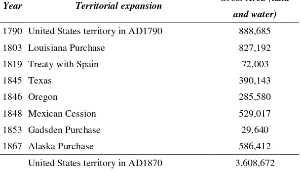
We might also consider how an exogenous increase in land supply could contribute to a “land expansion effect” on structural transformation. Such effect might have contributed to agricultural-to-manufacturing transformation in the United States during AD1790-AD1870. See Appendix 2 for details.

17

(53) max{ 𝑐𝑐̃𝑡𝑡, 𝐾𝐾_𝑡𝑡}∞_𝑡𝑡=0∫ 𝑒𝑒−(𝜌𝜌−𝑛𝑛)𝑡𝑡�𝑐𝑐̃𝑡𝑡

1−𝜃𝜃₋₁

1−𝜃𝜃 �

∞

0 𝑑𝑑𝑡𝑡 , subject to

(54) 𝐾𝐾̇_𝑡𝑡=Φ(𝐾𝐾_𝑡𝑡,𝑡𝑡)− 𝛿𝛿𝐾𝐾_𝑡𝑡− 𝑒𝑒𝑛𝑛𝑡𝑡𝐿𝐿₀𝑐𝑐̃_𝑡𝑡 ,

where Φ(𝐾𝐾_𝑡𝑡,𝑡𝑡) is the maximized value of current output at time 𝑡𝑡 (equation (34)), which is a function of the capital stock at time 𝑡𝑡:

Φ(𝐾𝐾_𝑡𝑡,𝑡𝑡)≡ max

𝐿𝐿𝐴𝐴𝑡𝑡,𝐿𝐿𝑀𝑀𝑡𝑡,𝐾𝐾𝐴𝐴𝑡𝑡,𝐾𝐾𝑀𝑀𝑡𝑡,𝑇𝑇𝐴𝐴𝑡𝑡,𝑇𝑇𝑀𝑀𝑡𝑡𝑌𝑌𝑡𝑡 , given 𝐾𝐾𝑡𝑡> 0 .

Note that Φ(𝐾𝐾_𝑡𝑡,𝑡𝑡) contains trending variables such as 𝐿𝐿_𝑡𝑡 and 𝑀𝑀_𝑡𝑡 (or 𝐴𝐴_𝑡𝑡), and sectoral shares

𝑙𝑙𝑀𝑀𝑡𝑡, 𝑘𝑘𝑀𝑀𝑡𝑡 and 𝜏𝜏𝑀𝑀𝑡𝑡 which evolve over time.28

Maximizing (53) subject to (54) is a standard optimal control problem. It yields the consumption Euler equation:

(55) 𝑐𝑐̃𝑡𝑡̇

𝑐𝑐̃𝑡𝑡=

1

𝜃𝜃[Φ𝐾𝐾− 𝛿𝛿 − 𝜌𝜌] ,

where Φ_𝐾𝐾 is the marginal product of capital of the maximized production function, which equals the capital rental 𝑅𝑅_𝑡𝑡 in the economy. Equations (55) and (54) characterize how per capita consumption composite and aggregate capital stock evolve over time.

To characterize the equilibrium dynamics of the system, we need to impose certain assumptions, appropriately normalize per capita consumption composite and aggregate capital stock, and include sectoral share evolution equations.29 For the first purpose, we assume that: (A1) 𝜀𝜀< 1 ,

(A2) 𝛽𝛽_𝑀𝑀>𝛽𝛽_𝐴𝐴 , (A3) 𝑔𝑔_A >�1−𝛽𝛽𝐴𝐴

1−𝛽𝛽𝑀𝑀� 𝑔𝑔𝑀𝑀+�𝛼𝛼𝑀𝑀− 𝛼𝛼𝐴𝐴+

𝛼𝛼𝑀𝑀(𝛽𝛽𝑀𝑀−𝛽𝛽𝐴𝐴)

1−𝛽𝛽𝑀𝑀 � 𝑛𝑛 .

Assumption (A1) states that agricultural and manufacturing goods are consumption complements. Assumption (A2) states that the manufacturing sector is the capital-intensive sector in the economy.

We denote �1−𝛽𝛽𝐴𝐴

1−𝛽𝛽𝑀𝑀� 𝑔𝑔𝑀𝑀 as the augmented manufacturing technology growth rate, and �𝛼𝛼𝑀𝑀− 𝛼𝛼𝐴𝐴+

𝛼𝛼𝑀𝑀(𝛽𝛽𝑀𝑀−𝛽𝛽𝐴𝐴)

1−𝛽𝛽𝑀𝑀 � 𝑛𝑛 as the augmented population growth rate. Assumption (A3) states that the agricultural technology growth rate is greater than the sum of augmented manufacturing technology growth rate and augmented population growth rate (we will explain this assumption in more detail in section 5.4). These three assumptions assure that the manufacturing sector is the asymptotically dominant sector.30

For the second purpose, we normalize per capita consumption composite and aggregate capital stock by population and productivity of the asymptotically dominant sector:

28

See equation (A.8) in Appendix 1 for the reduced-from expression of Φ(𝐾𝐾_𝑡𝑡,𝑡𝑡).

29

Mathematically, we want to remove the trending terms in (54)-(55) and include a sufficient number of equations to capture the evolution of per capita consumption composite, aggregate capital stock and sectoral shares in an autonomous system of differential equations.

30

We adopt Acemoglu and Guerrieri (2008, 479)’s notation that “[t]he asymptotically dominant sector is the sector that determines the long-run growth rate of the economy.”

18

(56) 𝑐𝑐_𝑡𝑡≡𝑐𝑐̃𝑡𝑡𝐿𝐿𝑡𝑡 1−𝛼𝛼𝑀𝑀−𝛽𝛽𝑀𝑀 1−𝛽𝛽𝑀𝑀 𝑀𝑀𝑡𝑡 1 1−𝛽𝛽𝑀𝑀 ,

(57) 𝜒𝜒_𝑡𝑡≡𝐾𝐾𝑡𝑡 1−𝛽𝛽𝑀𝑀

𝛼𝛼𝑀𝑀

𝐿𝐿𝑡𝑡𝑀𝑀𝑡𝑡 1 𝛼𝛼𝑀𝑀 .

With these two normalized variables, given the initial conditions 𝜒𝜒₀ and 𝑘𝑘_𝑀𝑀0, we can characterize the equilibrium dynamics of the economy by an autonomous system of three differential equations in 𝑐𝑐_𝑡𝑡, 𝜒𝜒_𝑡𝑡 and 𝑘𝑘_{𝑀𝑀𝑡𝑡}, as stated in proposition 7.

Proposition 7 (Equilibrium dynamics): Suppose (A1)-(A3) hold. The equilibrium

dynamics of the economy is characterized by the following three differential equations:

(58) 𝑐𝑐̇𝑡𝑡

𝑐𝑐𝑡𝑡=

1

𝜃𝜃�𝜔𝜔𝑀𝑀𝛽𝛽𝑀𝑀𝜂𝜂𝑡𝑡

1

𝜀𝜀𝜒𝜒_𝑡𝑡−𝛼𝛼𝑀𝑀𝑅𝑅𝛾𝛾𝑀𝑀_𝑙𝑙

𝑀𝑀𝑡𝑡𝛼𝛼𝑀𝑀𝑘𝑘𝑀𝑀𝑡𝑡𝛽𝛽𝑀𝑀−1𝜏𝜏𝑀𝑀𝑡𝑡𝛾𝛾𝑀𝑀− 𝛿𝛿 − 𝜌𝜌� −_1−𝛽𝛽𝑔𝑔𝑀𝑀_𝑀𝑀+�1−𝛼𝛼_1−𝛽𝛽𝑀𝑀−𝛽𝛽_𝑀𝑀𝑀𝑀� 𝑛𝑛 ,

(59) 𝜒𝜒̇𝑡𝑡

𝜒𝜒𝑡𝑡=

1−𝛽𝛽𝑀𝑀

𝛼𝛼𝑀𝑀 �𝜂𝜂𝑡𝑡𝜒𝜒𝑡𝑡

−𝛼𝛼𝑀𝑀_𝑅𝑅𝛾𝛾𝑀𝑀_𝑙𝑙

𝑀𝑀𝑡𝑡𝛼𝛼𝑀𝑀𝑘𝑘𝑀𝑀𝑡𝑡𝛽𝛽𝑀𝑀𝜏𝜏𝑀𝑀𝑡𝑡𝛾𝛾𝑀𝑀− 𝜒𝜒𝑡𝑡−

𝛼𝛼𝑀𝑀

1−𝛽𝛽𝑀𝑀_{∙ 𝑐𝑐𝑡𝑡− 𝛿𝛿� − 𝑛𝑛 −}𝑔𝑔𝑀𝑀

𝛼𝛼𝑀𝑀 ,

(60) 𝑘𝑘̇𝑀𝑀𝑡𝑡

𝑘𝑘𝑀𝑀𝑡𝑡=

(1−𝑘𝑘𝑀𝑀𝑡𝑡)�(𝑔𝑔𝑀𝑀−𝑔𝑔𝐴𝐴)+(𝛼𝛼𝑀𝑀−𝛼𝛼𝐴𝐴)𝑛𝑛+(𝛽𝛽𝑀𝑀−𝛽𝛽𝐴𝐴)�_{1−𝛽𝛽𝑀𝑀}𝛼𝛼𝑀𝑀 𝜒𝜒̇𝑡𝑡_{𝜒𝜒𝑡𝑡}+_{1−𝛽𝛽𝑀𝑀}𝛼𝛼𝑀𝑀 𝑛𝑛+_{1−𝛽𝛽𝑀𝑀}𝑔𝑔𝑀𝑀 �� �_𝜀𝜀−1𝜀𝜀 �−[(𝛽𝛽𝑀𝑀−𝛽𝛽𝐴𝐴)(1−𝑘𝑘𝑀𝑀𝑡𝑡)+(𝛼𝛼𝑀𝑀−𝛼𝛼𝐴𝐴)(1−𝑙𝑙𝑀𝑀𝑡𝑡)+(𝛾𝛾𝑀𝑀−𝛾�