Munich Personal RePEc Archive
Bayesian Inference in a
Non-linear/Non-Gaussian Switching
State Space Model: Regime-dependent
Leverage Effect in the U.S. Stock Market
Kim, Jaeho
University of Oklahoma
9 October 2015
Online at
https://mpra.ub.uni-muenchen.de/67579/
Bayesian Inference in a Non-linear/Non-Gaussian Switching State Space Model: Regime-dependent Leverage Effect in the U.S. Stock Market
Jaeho Kim∗
University of Oklahoma
This version: Oct, 2015
Abstract
This paper provides a Bayesian algorithm to efficiently estimate non-linear/non-Gaussian
switching state space models by extending a standard Particle Markov chain Monte Carlo
(PM-CMC) method. Instead of iteratively running separate PMCMC steps, the proposed particle
Gibbs sampler generates continuous-state and discrete-regime indicator variables together from
their joint smoothing distribution in one Gibbs block. The proposed Bayesian algorithm that is
built upon the novel idea of ancestor sampling is robust to small numbers of particles. Moreover,
the algorithm is applicable to any switching state space models, regardless of the Markovian
property. The difficulty in conducting Bayesian model comparisons is overcome by adopting
the Deviance Information Criterion (DIC). For illustration, a conventional regime switching
stochastic volatility model is generalized to encompass the regime-dependent leverage effect and
is applied to Standard and Poor’s 500 and NASDAQ daily return data. The resulting Bayesian
posterior estimates based on the proposed method indicate that the stronger (weaker) financial
leverage effect is associated with a high (low) volatility regime.
Keywords: Particle Markov Chain Monte Carlo, Regime switching, State space model, Leverage
effect
JEL classification: C11, C15
∗Department of Economics, University of Oklahoma, Norman, OK 73019, U.S.A. [E-mail: [email protected]]
I gratefully acknowledge financial support through the Junior Faculty Research Program at the University of
1
Introduction
The dynamics of many economic and financial time series often dramatically change, in
associ-ation with important economic events, such as economic policy changes, economic recessions, and
financial crises. Since the seminar article by Hamilton (1989), numerous studies have statistically
handled such abrupt changes in fundamental economic structures. In particular, linear/Gaussian
switching state space models (LG-SSSMs) have been of great use in the economic literature due to
their flexibility in encompassing a broad range of economic models1. However, though LG-SSSMs
have been proved to be quite useful in the literature, they have some drawbacks. Most importantly,
they impose linearity and Gaussianity assumptions that are too restrictive to handle
fundamen-tally non-linear economic variables with non-Gaussian innovations. On this ground, it is important
to develop an efficient method to estimate the novel class of non-linear/non-Gaussian switching
state space models (NLG-SSSMs), and this paper attempts to achieve this goal by extending the
standard Particle Markov Chain Monte Carlo method (PMCMC) by Andrieu et al. (2010).
A main difficulty in estimating NLG-SSSMs is that latent continuous-state and discrete-regime
indicator variables that drive a dynamic system usually have high dimensions and complicated
dependence patterns. Consequently, no closed-form expression exists in most cases for the posterior
distributions of unknown parameters. The PMCMC method is an simulation-based algorithm
which numerically approximates the posterior distributions of interest using random samples called
‘particles’. The method employs a sequential Monte Carlo (SMC) algorithm, also known as a
particle filter, to construct proposal kernels for an MCMC sampler. In this paper, I particularly
focus on developing an efficient particle Gibbs (PG) sampler for NLG-SSSMs, which is one kind of
the PMCMC method described by Andrieu et al. (2010). Another important class of the PMCMC
method, a particle marginal Metropolis-Hastings (PMMH) sampler, may be easily derived based
on the results provided in this paper.
The standard PG sampler by Andrieu et al. (2010) is first extended to accommodate regime
changes in a non-linear dynamic system. This basic algorithm is treated as a benchmark PG
algorithm throughout this paper. A modified sequence Monte Carlo (SMC) method is derived to
incorporate a regime indicator variable, which targets the joint smoothing distribution of the whole
sequence of the continuous state and the regime indicator variables. However, the approximate
joint smoothing distribution obtained by the proposed SMC method is unreliable, which in turn
produces MCMC output that mixes poorly. This problem is mainly caused by path degeneracy.
Path degeneracy refers to a phenomenon by which most of particle trajectories tends to collapse
to a single path as the SMC is operated forward in time. Andrieu et al. (2003) and Driessen
and Boers (2005) documented that when a dynamic system depends on dramatic regime changes,
path degeneracy becomes more severe. While increasing the number of particles can mitigate path
degeneracy, it may induce huge computation costs because the modified SMC is to be performed
at every MCMC iteration.
I introduce an alternative PG sampler that is robust to path degeneracy building on the idea of
Whiteley (2010). In the proposed sampler, I implicitly incorporate additional backward recursion
to the modified SMC method by employing ancestor sampling as described by Lindsten and Schon
(2012) and Lindsten et al. (2014). The ancestor sampling step is designed to increase the number
of unique particles by re-shuffling the previous particle trajectories in an existing particle swarm.
By preventing path degeneracy, the PG with ancestor sampling therefore significantly improves
the approximation of the joint smoothing distribution ofxt and st. As a result, the proposed PG
sampler achieves satisfactory mixing with a reasonably small number of particles.
An important feature of the proposed PG sampler with ancestor sampling is to sequentially
generates the continuous state and the discrete regime indicator variables together from their joint
smoothing distribution, in contrast to the conventional approaches, which iteratively run separate
PMCMC steps. The joint sampling can be effectively done in one Gibbs block by exploiting the
hierarchical structure of NLG-SSSMs. Properly designed MCMC kernels in the new approach target
the joint posterior distribution. Therefore, the dependence between the continuous-state and the
discrete-regime indicator variables does not affect the mixing properties of the resulting sampler.
A prominent example in which the continuous state and the discrete regime indicator variables are
perfectly correlated is provided by the Bayesian change-point models in Pesaran et al. (2006) and
is generated in one Gibbs block conditional on the regime indicator variable and then the regime
indicator variable is generated in another block conditional on the continuous state. However, this
sampling scheme does not converge to the correct stationary distribution as it is degenerate for the
change-point models.
Also, I note that the proposed PG sampler is a multi-move sampler in terms of the regime
indicator variable. The theoretical results by Liu et al. (1994) and Scott (2002) suggest that a
single-move sampler produces highly autocorrelated MCMC outputs for the regime indicator variable and
other model parameters. Kim and Kim (2014) also empirically showed that a single-move sampler
is undesirable in the sense that it fails to converge to a correct stationary distribution when the
regime indicator variable is highly persistent or has absorbing states. The proposed PG sampler
in this paper is completely free from those problems caused by a single-move sampling approach.
Furthermore, the proposed method can be easily applied to general NLG-SSSMs regardless of the
Markovian property.
There are several works in the literature related to this paper. For instance, Flury and Shephard
(2011) developed a PMCMC algorithm using a Particle Marginal Metropolis-Hastings (PMMH)
approach and apply it to three popular economic models. Even though a PMMH algorithm can
be developed for Bayesian inference of NLG-SSSMs based on the results presented in section 2,
convergence of their sampler may be very slow especially without a large number of particles2.
Of cause, one may achieve satisfactory convergence by increasing the number of particles, which is
computationally very demanding for complex dynamic models. Moreover, since a PMMH algorithm
often employs random walk proposals in generating model parameters, many of candidates will be
wasted due to low acceptance probabilities.
Nonejad (2014) recently proposed a PMCMC method based on a Gibbs sampling approach to
estimate a special class of NLG-SSSMs that this paper handles. The proposed method is
imple-mented by first drawing a continuous state variable, sayxt, given a regime indicator variablestand
then drawing the regime indicator variablest without conditioning onxt in the second step. The
2Pitt et al. (2012) provided theoretical results on the important trade-off between the convergence performance
second step of the algorithm generates st simply by replacing the true likelihood with the
approx-imate likelihood using a SMC method to integrate out xt. However, because the approximation
errors generated by a SMC method are completely ignored, the errors will introduce some bias by
propagating through the resulting MCMC sampler. Song (2014) developed a PMMH algorithm by
exploiting the partially linear structure of a switching state space model and incorporating Kim’s
(1994) approximate filtering and smoothing algorithms. An efficient PG algorithm was also
pro-posed by Whiteley et al. (2010) to estimate linear/Gaussian SSSM. While the existing algorithms
are potentially very useful for many applications, they are either computationally inefficient or not
directly applicable to this article because the empirical models of U.S. stock returns in Section 4
involve fully non-linear transition and measurement equations and the regime indicator variable is
indeed highly persistent in actual data.
Importantly, Mendes et al. (2014) suggested a general PMCMC scheme by properly combining
PMMH and PG methods. More specifically, PG steps are employed to generate the model
param-eters that are only weakly correlated with the latent states and then, separate PMMH steps are
performed for posterior simulation on the model parameter that are strongly correlated with the
state variables. With the proposed PG algorithm in this paper, one may be able to easily obtain a
further advanced PMCMC scheme for many NLG-SSSMs following Mendes et al. (2014).
For empirical illustration, I investigate the relationship between volatility and return in the U.S.
stock markets in the presence of regime switching by employing the econometric tool developed.
A conventional regime switching stochastic volatility (RS-SV) model is generalized to encompass
regime-dependent leverage effect and is applied to S&P 500 and NASDAQ daily return data. The
main idea behind this modeling approach is that when a leverage ratio which represents a firm’s
financial status is high, the firm becomes more venerable to a shock to its equity return. Because
a high leverage ratio is typically associated with high stock volatility, in times of high return
volatility, the response of volatility to a return shock should be larger than in normal times with
relatively lower return volatility. This asymmetric response of volatility across different volatility
regimes is the empirical feature that the proposed SV model is intended to capture. Some recent
leverage effect. Especially, Bandi and Ren`o (2012) theoretically illustrated this mechanism and
developed a non-parametric estimation method for time-varying leverage effect. Building upon
what has been suggested in the literature, this paper provides a new regime switching SV model
with regime-dependent leverage effect to further investigate this important empirical issue.
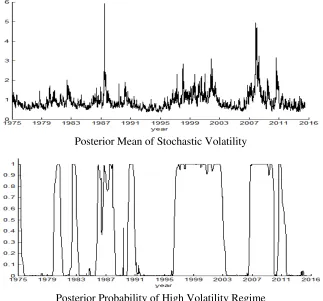
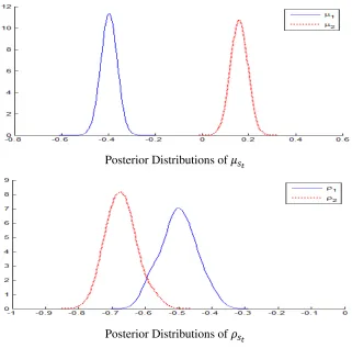
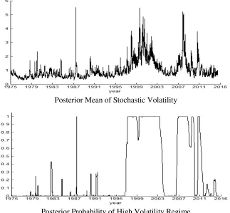
The new RS-SV model is applied to daily stock returns from the first week of January 1975
to the first week of August 2015. The Bayesian posterior means of the correlation parameters
turn out to be significantly different across high- and low-volatility regimes, which we originally
conjecture. In particular, the Bayesian estimates indicate that the stronger (weaker) leverage effect
is associated with a high (low)-volatility regime. Based on the Deviance Information Criterion
(DIC) by Spiegelhalter et al. (2002), it is shown that the models with the regime-dependent
leverage effect are always preferred to those with the constant leverage effect, regardless of the
number of regimes. This empirical results are consistent with the time-varying leverage effect in
the U.S. stock market described by Bandi and Ren`o (2012).
The organization of the paper is given as follows. In Section 2, I introduce model specification
and derive a modified sequential Monte Carlo algorithm for a general NLG-SSSM. Section 3 provides
details of the proposed PG sampler and a model selection criterion. The performance of the
new algorithm is also illustrated using simulated data. In Section 4, I demonstrate the proposed
technique on data from the U.S. stock market. Concluding remarks are provided in Section 5.
2
Model Specification and Particle Filtering
2.1 Model Specification
Non-linear/non-Gaussian Switching State-Space Models (NLG-SSSM) are a class of models in
which the structure and the parameters of a non-linear state-space model switch according to
discrete latent processes3. A state space model consists of the measurement equationF(.) and the
transition equationH(.):
yt=Fs0:t(x0:t, ǫt) (1)
xt=Hs0:t(x0:t−1, ut)
where the dynamic system is observed over a time intervalt= 1,2, ..., T;xt∈X is the unobserved
state vector; Yt ∈ Y is the observation vector; x0:t = {x0, x1, ..., xt}, and s0:t = {s0, s1, ..., st};
and ut and ǫt are identically distributed random variables with zero means and are not serially
correlated4. The properties of the state space model such as dimensions, functional forms, and
model parameters shift over time according to a set of discrete latent variabless0:t={s0, s1, ..., st}.
The NLG-SSSM is parameterized by unknown parametersβst, subject to the discrete latent variable
st. The latent variablestfollows a K-state first-order Markov switching process with the following
transition probabilities:
p(st=j|st−1 =k) =πkj, K
X
j=1
πkj = 1, i, k= 1,2, ..., K. (2)
The model parameters under K-regimes and the transition probabilities are denoted by θ =
{β1, β2, ..., βK, π} ∈Θ. The hierarchical structure of the non-linear/non-Gaussian SSSM specified
by equations (1) and (2) is the main difference from that of a canonical non-linear/non-Gaussian
state-space model with discrete states. The distributions of the initial states are associated with
the prior densities gθ(x0, s0) =gθ(x0|s0)gθ(s0). Note that the above NLG-SSSM does not possess
the Markovian property. Although the measurement and transition equations often depend on just
a few latent states in practice, I adhere to the general model specification throughout this paper
for generality of exposition.
Our primary concern in this article is to perform Bayesian inference in an NLG-SSSM. The two
sets of latent variables x0:T = {x0, x1, ..., xT}, s0:T = {s0, s1, ..., sT} and the model parameters θ
are treated as unknowns and jointly estimated based on the posterior density given as:
p(θ, x0:T, s0:T|Y1:T)∝
T
Y
t=1
fθ(yt|x0:t, s0:t)gθ(xt|x0:t−1, s0:t)gθ(st|st−1)
gθ(x0|s0)gθ(s0)π(θ) (3)
where fθ(.) and gθ(.) denote probability densities associated with equations (1) and (2), given θ;
π(θ) is the prior density of θ. Because the posterior is not available in closed form, Bayesian
inference is often infeasible without simulation-based methods.
4The functions
F(.) andH(.) can contain additional exogenous variables, but potential exogenous variables are
2.2 Particle Filtering for a Non-linear/Non-Gaussian SSSM
To develop an efficient particle Gibbs algorithm, it is crucial to sample from the joint smoothing
distribution of the latent state variables conditional on y1:T = {y1, y2, ..., yT}. First, consider the
following useful decomposition of the joint filtering densitypθ(x0:t, s0:t|y1:t):
pθ(x0:t, s0:t|y1:t) =pθ(xt, x0:t−1, st, s0:t−1|yt, y1:t−1)
= pθ(yt, xt, x0:t−1, st, s0:t−1|y1:t−1) pθ(yt|y1:t−1)
= fθ(yt|x0:t, s0:t)gθ(xt|x1:t−1, s0:t)gθ(st|st−1) pθ(yt|y1:t−1)
pθ(x0:t−1, s0:t−1|y1:t−1).
(4)
Note the joint smoothing densitypθ(x0:T, s0:T|y1:T) of our interest can be obtained according to the
recursive structure in equation (4) ast=T. While evaluating the exact joint filtering density is a
very difficult task because of analytically non-tractablepθ(x0:t−1, s0:t−1|y1:t−1) andfθ(yt|y1:t−1), we
can properly approximate the joint filtering density in equation (4) using random samples called
‘particles’. Gordon et al. (1993) originally developed a particle filtering method to recursively
approximate a filtering density of continuous latent state variables. It is worth mentioning that
the standard particle filter described by Gordon et al. (1993) can be considered a special case of
the popular auxiliary particle filter of Pitt and Shephard (1999). These particle filters are also
known as sequential Monte Carlo (SMC) methods. In this section, the standard particle filters are
extended and applied to obtain the approximate joint filtering and smoothing densities of xt and
stin a NLG-SSSM.
Let{X0:t, S0:t}={x(0:i)t, s
(i)
0:t}Ni=1denote a set of particles, in whichN represents the total number of particles. The N particles are generated from the following importance distribution in an SMC
method for a NLG-SSSM:
q(x0:t, s0:t) =q(xt|x0:t−1, s0:t)q(st|x0:t−1, s0:t−1)q(x0:t−1, s0:t−1) (5)
where q(.)’s denote importance densities possibly depending upon y1:t. Equation (5) implies that
new states{x(ti), st(i)} are sequentially generated from q(st|x0:t−1, s0:t−1) and q(xt|x0:t−1, s0:t)
con-ditional on the corresponding past sequence{x(0:i)t−1, s(0:i)t−1}fromq(x0:t−1, s0:t−1) fori= 1,2, ..., N.
set of particle trajectories {X0:(i)t, S0:(i)t} ={x(0:i)t, s(0:i)t}N
i=1. A candidate distribution to generate new particles at timetis referred to as an incremental importance distribution.
As an importance distribution is usually not identical to the target distribution, we need to
correct the corresponding approximations by imposing importance weights to generated particles
as:
ωt(i)= pθ(x (i) 0:t, s
(i) 0:t|y1:t)
q(x(0:i)t, s(0:i)t)
= fθ(yt|x (i) 0:t, s
(i)
0:t)gθ(x(ti)|x
(i) 0:t−1, s
(i)
0:t)gθ(s(ti)|s
(i)
t−1) pθ(yt|y1:t−1)q(x(ti)|x
(i) 0:t−1, s
(i) 0:t)q(s
(i)
t |x
(i) 0:t−1, s
(i) 0:t−1)
pθ(x(0:i)t−1, s (i)
0:t−1|y1:t−1) q(x(0:i)t−1, s(0:i)t−1)
∝ fθ(yt|x (i) 0:t, s
(i) 0:t)gθ(x(
i)
t |x
(i) 0:t−1, s
(i) 0:t)gθ(s(
i)
t |s
(i)
t−1) q(x(ti)|x0:(i)t−1, s(0:i)t)q(s(ti)|x(0:i)t−1, s(0:i)t−1) ω
(i)
t−1
∝ω¯t(i)ωt(−i)1
(6)
for i= 1,2, ..., N. The first term ¯ωt(i) in equation (6) is called an incremental importance weight.
Suppose that the estimate of the importance weight ωt−1 at t−1 is available and is denoted by
ˆ
ωt−1. Then, because the importance weightωt(i)is only proportional to ¯ω
(i)
t ω
(i)
t−1 due to the unknown normalizing constantpθ(yt|y1:t−1), our estimate of the importance weightωt(i) attis obtained as:
ˆ
ω(ti)= ω¯ (i)
t ωˆ
(i)
t−1
PN
j=1ω¯ (j)
t ωˆ
(j)
t−1
through self-normalization. Moreover, we can approximately evaluate the likelihood function as:
ˆ
pθ(y1:t) = t
Y
l=1 ˆ
pθ(yl|yl−1) =
t Y l=1 N X i=1 ¯
ωl(i)ωˆl(−i)1. (7)
The approximate likelihood value obtained running a SMC procedure is a key ingredient for a
PMMH algorithm and some model comparison criteria.
It is well know that a filtering algorithm without a re-sampling step seriously suffers from weight
degeneracy. Weight degeneracy represents a phenomenon that most of the particles trajectories
{X0:t−1, S0:t−1} = {x(0:i)t, s
(i)
0:t}Ni=1 diverge from their true latent states over time, increasing the variance of importance weights, and all importance weights eventually converge to zero except only
(1999) to prevent weight degeneracy, I include a re-sampling step in which N random particles
{˜x(0:i)t,s˜(0:i)t}N
i=1are re-drawn from the existing particles{x (i) 0:t, s
(i)
0:t}Ni=1with the normalized importance weight{ωˆt(i)}Ni=1. The role of the additional re-sampling step is to replicates probable particles with
high importance weights. In contrast, it eliminates unlikely particles with low importance weights to
avoid path degeneracy. Because the re-sampling step allows us to obtain equally weighted particles
approximately distributed from pθ(x0:t, s0:t|y1:t), a new set of weights {ω˜(ti) = N1}Ni=1 is assigned
to the re-sampled particles {˜x(0:i)t,˜s(0:i)t}N
i=1. In what follows, I provide the summary of the SMC algorithm for a NLG-SSSM.
Algorithm 1-1: Sequential Monte Carlo (SMC)
i) Draw{s(0i)}N
i=1fromq(s0) and draw{x(0i)}Ni=1fromq(x0|s(0i)). Save the normalized importance weights{ωˆ(0i)= ω¯(
i) 0
PN j=1ω¯
(i) 0
}N
i=1 where ¯ω (i) 0 =
pθ(x(0i)|s0(i))pθ(s(0i))
q(x(0i)|s0(i))q(s(0i)) . • Iterate step ii), iii), and vi) fort= 1,2, ..., T.
ii) Resample N particles {x˜(0:i)t−1,˜s(0:i)t−1}N
i=1 from {x (i) 0:t−1, s
(i)
0:t−1}Ni=1 with probability {ˆω (i)
t−1}Ni=1 and assign new importance weights{ω˜(t−i)1 = N1}Ni=1. Rename the particles {˜x0:(i)t−1,˜s0:(i)t−1}Ni=1
into{x(0:i)t−1, s(0:i)t−1}N
i=1 and the importance weights {˜ω (i)
t−1}Ni=1 into {ω (i)
t−1}Ni=1. iii) Draw{s(ti)}N
i=1fromg(s (i)
t |x
(i) 0:t−1, s
(i)
0:t−1) and draw{x (i)
t }Ni=1fromg(x (i)
t |x
(i) 0:t−1, s
(i)
0:t). Set{x
(i) 0:t}Ni=1= {x(0:i)t−1, xt(i)}Ni=1 and {s(0:i)t}Ni=1={s(0:i)t−1, s(ti)}Ni=1.
vi) Calculate the unnormalized weights ¯ωt(i)ωˆt(−i)1 = fθ(yt|x(0:i)t,s
(i)
0:t)pθ(x(ti)|x
(i) 0:t−1,s
(i)
0:t)pθ(s(ti)|s
(i)
t−1)
q(x(ti)|s(0:i)t
−1,s
(i) 0:t)q(s
(i)
t |x
(i) 0:t−1,s
(i) 0:t−1)
ˆ
ωt(−i)1 and
obtain the normalized weights ˆωt(i)= ω¯
(i)
t ωˆ
(i)
t−1
PN j=1¯ω
(j)
t ωˆ
(j)
t−1
fori= 1,2, ..., N.
In fact, the estimate ˆωt−1 is always N1 for all time periods after re-sampling. Thus, one may
safely ignore ˆωt(−i)1 in calculating the normalized weights as ˆωt(i) = ω¯
(i)
t PN
j=1ω¯ (j)
t
. In the proposed SMC
procedure, the importance sampling is repeatedly operated at each time period to generate various
particle realizations {x(0:i)T, s(0:i)T}N
i=1 from pθ(x0:T, s0,T|y1:T). The target joint smoothing density is
approximated by:
pθ(x0:T, s0,T|y1:T)≈ N
X
i=1 ˆ ωT(i)δ
{x(0:i)T,s0:(i)T}(x0:T, s0:T) (8) whereδ
particle trajectory in{x(0:i)T, s(0:i)T}N
i=1. Accordingly, we can draw random samples from{x (i) 0:T, s
(i) 0:T}Ni=1 with the normalized weight{ˆωT(i)}N
i=1to simulate from the joint smoothing distributionpθ(x0:T, s0,T|y1:T).
Algorithm 1-2: Forward Filtering for pθ(x0:T, s0:T|y1:T)
• Run Algorithm 1-1 (SMC algorithm)and save the particle set {x0:(i)T, s(0:i)T}N
i=1 along with the normalized importance weights{ωˆT(i)}N
i=1 at timeT. i) Draw {˜x(0:jT),˜s(0:jT)}M
j=1 from {x (i) 0:T, s
(i) 0:T}
N
i=1 according to the normalized importance weights {ωˆT(i)}N
i=1.
2.3 Importance Distribution
When re-sampling xt and st in the SMC procedure, we inevitably discard many past particle
trajectories in{x(0:i)t, s(0:i)t}N
i=1, decreasing the number of unique particles at each time period. Conse-quently, the resulting particle paths in{x(0:i)T, s(0:i)T}N
i=1 at the terminal time period become sharing just a few common ancestors. This phenomenon called ‘path degeneracy’ results in a poor
ap-proximation of the joint smoothing densitypθ(x0:T, s0:T|y1:T). Andrieu et al. (2003) and Driessen
and Boers (2005) empirically demonstrated the path degeneracy problem gets worse when a
dy-namic system is subject to a discrete regime-indicator variable. Importantly, we will see that the
path degeneracy seriously deteriorates mixing of a PMCMC sampler. Even if an increase in the
number of particles can mitigate path degeneracy, huge computation costs are required when it is
implemented in a PMCMC algorithm.
Andrieu et al. (2003) and Driessen and Boers (2005) emphasized that the incremental
im-portance distributions q(xt|x0:t−1, s0:t) and q(st|x0:t−1, s0:t−1) in equation (5) should be carefully
designed to closely approximate the target joint filtering and smoothing densities to avid path
de-generacy. Following Pitt and Shephard (1999), we consider the following incremental importance
distribution that takes all available information ony1:t into account:
q(xt, st|x0:t−1, s0:t−1) =pθ(xt, st|x0:t−1, s0:t−1, y1:t)pθ(yt|x0:t−1, s0:t−1, y1:t−1) (9)
in generating the new states{x(ti), s(ti)}. The first component can be decomposed into two parts:
where:
pθ(st|x0:t−1, s0:t−1, y1:t) =
pθ(st, yt|x0:t−1, s0:t−1, y1:t−1) pθ(yt|x0:t−1, s0:t−1, y1:t−1))
∝pθ(st, yt|x0:t−1, s0:t−1, y1:t−1)
=pθ(yt|x0:t−1, s0:t, y1:t−1)pθ(st|x0:t−1, s0:t−1, y1:t−1)
∝pθ(yt|x0:t−1, s0:t, y1:t−1)gθ(st|st−1).
(10)
The validity of going from the second line to the third line is that all the past information ony1:t−1,
and x0:t−1 is not relevant for st conditional on st−1. The density pθ(yt|x0:t−1, s0:t, y1:t−1) is given
by:
pθ(yt|x0:t−1, s0:t, y1:t−1) = Z
fθ(yt|x0:t, s0:t, y1:t−1)pθ(xt|x0:t−1, s0:t, y1:t−1)dxt
Finally, the second term in (9) is given by:
pθ(yt|x0:t−1, s0:t−1, y1:t−1) = X
st
pθ(yt|x0:t−1, s0:t, y1:t−1)gθ(st|st−1)
Note that pθ(yt|x0:t−1, s0:t, y1:t−1) is not analytically tractable in general and thus, the density
should be approximated to construct the incremental importance density in equation (9).
Wan and van der Merwe (2001) advocated using a unscented Kalman filter (UKF) in a SMC
procedure especially when it is not possible to directly draw latent states from an importance
distribution. To build an importance distribution closer to a target distribution, their approach is
to transform a non-linear/non-Gaussian dynamic system into an approximate linear one through a
UKF. Similarly, we can adopt the modified UKF by Andrieu et al. (2003) to obtain an approximate
importance distribution in equation (9) to partially resolve path degeneracy in a NLG-SSSM.
The critical problem of this approach, however, is that the modified UKF for a NLG-SSSM
should be run for each particle at every time period, which exponentially increases computing time
for the algorithm. I confirm via a set of simulations that the computational costs of sampling from
the importance distribution in (9) far exceed its benefits from partially solving path degeneracy,
especially when it is incorporated in a PMCMC sampler. For this reason, we exploit the transition
densities associated with equations (1) and (2) and ignore information iny1:t as:
q(xt|x0:t−1, s0:t) =gθ(xt|x0:t−1, s0:t),
q(st|x0:t−1, s0:t−1) =gθ(st|st−1).
in constructing importance distributions forxt and st. The incremental importance distributions
in equation (11) are employed in forward filtering for all simulations and applications throughout
this paper.
Instead of improving the importance distributions ofxtandstused in forward filtering, we can
effectively address the problem of path degeneracy by implicitly complementing forward filtering
with additional backward smoothing for a NLG-SSSM. Based on the idea of Godsill et al.(2004), an
SCM algorithm with additional backward simulation can substantially alleviate path degeneracy by
shuffling existing particle trajectories backward in time. The advantage of this approach lies on the
fact that it exploits all the generated particles through forward filtering rather than discarding them.
This important feature of a backward smoothing algorithm is the key to successfully developing an
efficient PG sampler in the next section.
3
Particle Markov Chain Monte Carlo Methods for a
non-linear/non-Gaussian SSSM
3.1 Artificial target distribution
This section introduces a Gibbs sampling method to drawx0:T ands0:T from their joint
ing distribution. The main difficulties in deriving a proper Gibbs sampler are that the joint
smooth-ing distribution shows complex patterns of dependence among the latent variables, and samplsmooth-ing
{x0:T, s0:T} directly from the joint smoothing distribution is not possible in general as a result of
non-linearity and non-Gaussianity. To resolve these problems, I adopt a PG sampling approach to
estimate a NLG-SSSM following Andrieu et al. (2010) and illustrate that the proposed PG sampler
performs well in practice. Like any other Gibbs samplers, unnecessary accept/reject steps are not
required, which produces mixing properties that are better than those of PMMH samplers.
To make a valid particle Gibbs sampler, I use an artificial target distribution Φ(.) that contains
all of the randomness generated by the SMC method in Algorithm 1-1. To design the artificial
the index variable of the ancestor at timet−1 for i-th particles {xt(i), s(ti)}:
At={a(ti)}Ni=1.
For example, ifx(5)t−1 ands(5)t−1are drawn in the re-sampling step for generatingx(ti)ands(ti), the index
variable becomesa(ti)= 5. Using the ancestor index, entire particle trajectories can be constructed
by tracing back to their ancestral lineages recursively:
x(0:i)t={x(a
(i)
t )
0:t−1, x (i)
t }={x
(a(a
(i)
t ) t−1 ) 0:t−2 , x
(a(ti))
t−1 , x (i)
t }=...
s(0:i)t={s(a
(i)
t )
0:t−1, s (i)
t }={s
(a(a
(i)
t ) t−1 )
0:t−2 , s (a(ti))
t−1 , s (i)
t }=...
for i= 1,2, ..., N. Using the ancestor index variables, the density of the SMC inAlgorithm 1-1 is
given by:
Φ(X0:T, S0:T, A1:T|θ) = N
Y
i=1
q(x(0i)|s0(i))q(s(0i))
T Y t=1 N Y i=1 ¯ ωt(−i)1 P
jω¯
(j)
t−1
q(x(ti)|x(a
(i)
t )
0:t−1, s (i) 0:t)q(s
(i)
t |x
(a(ti)) 0:t−1, s
(a(ti)) 0:t−1)
=
N
Y
i=1
q(x(0i)|s0(i))q(s(0i))
T Y t=1 N Y i=1
Mtθ(a(ti), xt(i), s(ti))
.
(12)
where the transition kernelMtθ(a(ti), x(ti), s(ti)) in equation (12) is defined as follows:
Mtθ(a(ti), xt(i), s(ti)) = ω¯ (i)
t−1 P
jω¯
(j)
t−1
q(x(ti)|x(a
(i)
t )
0:t−1, s (i) 0:t)q(s
(i)
t |x
(a(ti)) 0:t−1, s
(a(ti)) 0:t−1),
and X0:T ={x(0:i)T}Ni=1; S0:T = {s0:(i)T}Ni=1; A1:T = {a(1:i)T}Ni=1; q(.) denote importance densities that
may depend ony1:t. The incremental importance weight ¯ωt(i) is given by:
¯
ωt(i)= fθ(yt|x (i) 0:t, s
(i)
0:t)pθ(x(ti)|x
(i) 0:t−1, s
(i)
0:t)pθ(s(ti)|s
(i)
t−1) q(x(ti)|x0:(i)t−1, s(0:i)t)q(s(ti)|x(0:i)t−1, s(0:i)t−1) .
fori= 1,2, ..., N. I note that the normalized importance weight ˆωt(i)= ¯ω
(i)
t ωˆ
(i)
t−1
P jω¯
(j)
t ωˆ
(j)
t−1
with whicha(ti+1)
is generated can be simplified to ˆωt(i) = ω¯
(i)
t P
jω¯
(j)
t
because we assign N1 to ˆωt(−i)1 after the resampling
step inAlgorithm 1-1. The incremental importance weight ¯ωt(i) is directly used in stead of ˆω(ti) in
Now, letK ∈ {1,2, ..., N}be the index of a fixed reference trajectory. For example, if we
gen-erate a single reference trajectory{x(10)0:T , s(10)0:T } from the joint smoothing distribution inAlgorithm
1-2, the index variable assumes K = 10. We can keep track of its ancestral lineage based on the
ancestor indice At ={a(ti)}Ni=1 for t = 1,2, ..., T. For the fixed reference trajectory, an additional index bt is introduced to describe the each particle in the reference trajectory for t = 1,2, ..., T.
The reference trajectoryx(0:KT) and s0:(KT) are equivalent represented with the index variablebt as:
x(b0:T)
0:T ={x
(b0)
0 , x (b1)
1 , ..., x (bT−1)
T−1 , x (bT)
T }
s(b0:T)
0:T ={s
(b0)
0 , s (b1)
1 , ..., s (bT−1)
T−1 , s (bT)
T }
According to the definition of bt, bt can be rewritten in terms of the ancestor index asbt=K for
t= T and bt=at(b+1t+1) fort = 0, ..., T−1. We often use K to denote the entire reference particle path andbt to denote its individual component. The introduced indices are all auxiliary variables
generated by the SMC procedure and will play a key role later in deriving valid MCMC transition
kernels.
Finally, the remaining latent states generated by the SMC procedure except the reference
tra-jectory with the index K or the sequence of indices b0:T ={b0, b1, ..., bT} are denoted by X0:(−Tb0:T)
and S(−b0:T)
0:T . Now, we can easily determine the conditional density of the SMC algorithm given a
reference trajectoryx(b0:T)
0:T and s
(b0:T)
0:T as follows:
Φ(X(−b0:T)
0:T ,S
(−b0:T)
0:T , A
(−b1:T)
1:T |θ, x
(b0:T)
0:T , s
(b0:T)
0:T , b0:T)
= Φ(X0:T, S0:T, A1:T|θ) q(x(b0)
0 |s (b0)
0 )q(s (b0)
0 )
QT
t=1
¯
ω(t−bt1) P
jω¯
(j)
t−1 q(x(bt)
t |x
(b0:t−1) 0:t−1 , s
(b0:t)
0:t )q(s
(bt)
t |x
(b0:t−1) 0:t−1 , s
(b0:t−1) 0:t−1 )
=
N
Y
i=1
i6=b0
q(x(0i)|s0(i))q(s(0i))×
T Y t=1 N Y i=1
i6=bt
Mtθ(a(ti), xt(i), s(ti))
(13)
defined by:
Φ(θ, X0:T, S0:T, A1:T, K)≡Φ(θ, x(0:bT0:T), s(0:b0:TT), b0:T)Φ(X0:(−Tb0:T), S0:(−Tb0:T), A1:(−Tb0:T)|θ, x0:(bT0:T), s0:(bT0:T), b0:T)
≡ 1
NT+1p(θ, x (b0:T)
0:T , s
(b0:T)
0:T |y1:T)
×
N
Y
i=1
i6=b0
q(x(0i)|s0(i))q(s(0i))×
T
Y
t=1
N
Y
i=1
i6=b0
Mtθ(a(ti), xt(i), s(ti))
(14)
where X0:T = {x( b0:T)
0:T , X
(−b0:T)
0:T }; S0:T = {s( b0:T)
0:T , S
(−b0:T)
0:T }; K ∈ {1,2, ..., N} is the index of a
reference trajectory. I develop an efficient particle Gibbs sampler in this section to estimate a
NLG-SSSM by targeting the extended target distribution in equation (14). As theoretically shown
by Andrieu et al. (2010), the new extended target distribution Φ(.) admits the original posterior
p(θ, x0:T, s0:T|y1:T) as a marginal. Therefore, a valid multi-step Gibbs sampler can be designed
based on Φ(.) to make reliable Bayesian inference in NLG-SSSMs.
3.2 Benchmark Particle Gibbs Sampler
We are interested in sampling fromp(θ, x0:T, s0:T|y1:T) based on a Particle Gibbs (PG) sampler.
By building a multi-stage Gibbs sampler including the auxiliary variables, I provide details of the
benchmark PG sampler which is a direct extension of the standard PG sampler by Andrieu et
al. (2010). The first step of the benchmark PG sampler is to sample the index K of a reference
trajectory. This is exactly the same as drawing one particular particle path from all generated
particle trajectories by the SMC method inAlgorithm 1-1. The conditional density for K is given
by:
Φ(K=k|θ, X0:T, S0:T, A1:T) =
¯ w(Tk)
PN
j=1w¯ (j)
T
(15)
based on the followingProposition 1.
Proposition 1 The conditional Φ(K|θ, X0:T, S0:T, A1:T) under the target Φ(θ, X0:T, S0:T, A1:T, K)
is proportional to the importance weight at T:
The proof ofProposition 1is based on Andrieu et al. (2010) and given in the Appendix B. According
to Proposition 1, it is straightforward to sample K from its conditional distribution in equation
(15).
As the second step, we sample θ based on a partially collapsed Gibbs step which marginalize
unnecessary random variables before conditioning in drawing θ. As shown by van Dyk and Park
(2008), this approach does not violate the invariance of the corresponding sampler. Under the
extended target distribution, the conditional distribution forθ is given by:
Φ(θ|x(b0:T)
0:T , s
(b0:T)
0:T , b0:T) =p(θ|x( b0:T)
0:T , s
(b0:T)
0:T , y1:T) (16)
Note that in practice, sampling θ from p(θ|x0:T, s0:T, y1:T) is so much simpler than sampling θ
conditional only on y1:T, For instance, the transition probabilities forst can be easily generated
from the beta distributions when using conjugate priors. When non-conjugate priors are used
or conditional posteriors do not belong to well-known distributions for some parameters, we can
employ Metropolis-Hastings algorithms within a Particle Gibbs sampling approach conditional on
x(b0:T)
0:T , s
(b0:T)
0:T . I assume that sampling θ from its conditional distribution under Φ(.) is
straight-forward by either using conjugate priors or Metropolis-Hastings algorithms given x(b0:T)
0:T , s
(b0:T)
0:T
throughout this paper.
The conditional distribution for the third step of the benchmark PG sampler is given by
Φ(X(−b0:T)
0:T , S
(−b0:T)
0:T , A
(−b1:T)
1:T |θ, x
(b0:T)
0:T , s
(b0:T)
0:T , b0:T) in equation (13). To achieve this goal, we
em-ploy a so-called conditional SMC algorithm. Simply speaking, the conditional SMC method is an
algorithm that generates new N −1 particle paths with the reference trajectory {x(b0:T)
0:T , s
(b0:T)
0:T }
fixed throughout the sampling process. As a matter of convenience, we set an alternative index
sequence for the reference particle path asb0:T ={N, N, ..., N}. This is because the index sequence
b0:T is just a convenient tool to locate each particle in the reference trajectory in the particle swarm
and thus their actual values do not matter at all in the conditional SMC procedure. The following
algorithm summarizes the conditional SMC method used in our benchmark PG sampler.
Algorithm 2-1: Conditional Sequential Monte Carlo (CSMC)
i) Draw{s(0i)}iN=1−1fromq(s0) and draw{x0(i)}Ni=1−1fromq(x0|s(0i)) sequentially. Set{x (N) 0 , s
{x(b0)
0 , s (b0)
0 }. Save the normalized importance weights {ωˆ (i) 0 =
¯
ω0(i) PN
j=1ω¯ (i) 0
}N
i=1 where ¯ω (i) 0 =
pθ(x( i) 0 |s
(i) 0 )pθ(s(
i) 0 )
q(x(0i)|s0(i))q(s(0i)) .
• Iterate step ii), iii), and vi) fort= 1,2, ..., T.
ii) Draw ancestor indices{a(ti)}iN=1−1with probability{ωˆt(−i)1}N
i=1. Draw{s (i)
t }Ni=1−1fromq(s (i)
t |x
(a(ti)) 0:t−1, s
(a(ti)) 0:t−1) and {x(ti)}iN=1−1 from q(x(ti)|x(a
(i)
t )
0:t−1, s (a(ti)) 0:t−1, s
(i)
t ) sequentially.
iii) Seta(tN)=N and{xt(N), s(tN)}={x(bt)
t , s
(bt)
t }. New trajectories are set byx
(i) 0:t={x
(a(ti)) 0:t−1, x
(i)
t }
and s(0:i)t={s(a
(i)
t )
0:t−1, s (i)
t }fori= 1,2, ..., N.
vi) Calculate the unnormalized weights: ¯ωt(i) =fθ(yt|x(0:i)t,s
(i)
0:t,y1:t−1)pθ(x(ti)|x
(a(ti)) 0:t−1,s
(i)
0:t)pθ(s(ti)|s
(a(ti))
t−1 )
q(x(ti)|x(a
(i)
t )
0:t−1,s
(i) 0:t)q(s
(i)
t |x
(a(i) t )
0:t−1,s
(a(i) t )
0:t−1)
.
and obtain the normalized weights: ˆωt(i)= ω¯
(i)
t PN
j=1ω¯ (i)
t
fori= 1,2, ..., N.
Note that sampling ancestor indices{a(ti)}Ni=1−1 in step ii) is equivalent to re-samplingN−1 particles
{˜x(t−i)1,˜st(i−)1}Ni=1−1 from {x(ti−)1, s(t−i)1}N
i=1 with probability {ωˆ (i)
t−1}Ni=1. This completes the benchmark PG sampler for a NLG-SSSM. The summary of the benchmark PG algorithm is given by the
following.
Algorithm 2-2: Benchmark PG for a Non-linear/non-Gaussian SSSM
Choose θ arbitrarily and draw {X0:T, S0:T, A1:T} by running Algorithm 1-1 (SMC
algo-rithm): {X0:T, S0:T, A1:T} ∼Φ(X0:T, S0:T, A1:T|θ)
• Iterate step i), step ii), and step iii) for r= 1,2, ..., R.
i) DrawK∈ {1,2, ..., N}(a reference trajectory) from: K ∼Φ(K|θ, X0:T, S0:T, A1:T)
And set{x(b0:T)
0:T , s
(b0:T)
0:T }={x
(K) 0:T, s
(K) 0:T}.
ii) Drawθfrom: θ∼Φ(θ|x(b0:T)
0:T , s
(b0:T)
0:T , b0:T)
iii) Draw{X(−b0:T)
0:T , S
(−b0:T)
0:T , A
(−b1:T)
1:T }by running Algorithm 2-1 (CSMC algorithm) from:
{X(−b0:T)
0:T , S
(−b0:T)
0:T , A
(−b1:T)
1:T } ∼Φ(X
(−b0:T)
0:T , S
(−b0:T)
0:T , A
(−b1:T)
1:T |θ, x
(b0:T)
0:T , s
(b0:T)
0:T , b0:T)
And setX0:T ={X0:(−Tb0:T), x
(b0:T)
0:T },S0:T ={S0:(−Tb0:T), s
(b0:T)
0:T },A1:T ={A1:(−Tb1:T), b0:T−1}.
In the summary, the variableK represents the index of a reference particle trajectory andR is the
Many papers such as those by Whiteley (2010), Fredrik and Schon (2012), and Whiteley et al.
(2011) recognize that a standard PG sampler by Andrieu et al. (2010) seriously suffers from poor
mixing due to path degeneracy. Moreover, Andrieu et al. (2003) and Driessen and Boers (2005)
showed that the path degeneracy problem becomes much serious with the presence of a regime
indicator variable in a dynamic system. In section 3.6, we will see that the benchmark PG sampler
indeed produces unsatisfactory performance when it is applied to a NLG-SSSM. To address the
issues regarding path degeneracy and poor mixing, I introduce an improved PG sampler in the next
section.
3.3 Proposed Particle Gibbs Sampler
The approximate joint smoothing distribution ofxt and st obtained using the SMC algorithm
inAlgorithm 1-1 is unreliable due to path degeneracy. As the SMC procedure is performed forward
in time, the number of unique particles significantly decreases as we discard many past particle
trajectories in the re-sampling step. Consequently, the particles set {x(0:i)t, s0:(i)t}Ni=1 share just a few
common ancestors, which inevitably leads to a poor approximation of the joint smoothing
distri-butionpθ(x0:T, s0:T|y1:T). Godsill et al.(2004) originally addressed the problem of path degeneracy
by complementing forward filtering with additional backward smoothing. A backward smoothing
algorithm allows us to exploit all of the generated particles at each time instead of wasting them.
This important feature of backward smoothing provides a successful way to develop an efficient PG
sampler.
A PG sampler with ancestor sampling (PGAS) developed by Fredrik and Schon (2012) and
Lindsten et al. (2014) implicitly incorporates the backward simulation by updating particle
trajec-tories forward in time. In this section, I propose a PGAS sampler for a NLG-SSSM that targets
the extended target distribution in equation (14) to resolve path degeneracy and improve mixing
of the resulting MCMC chain based on the works of Fredrik and Schon (2012) and Lindsten et al.
(2014). The main difference between the proposed PG sampler and the benchmark PG sampler is
in the treatment of the index variables b0:T−1 ={b0, b1, ..., bT−1} of a reference trajectory. While
the proposed PG sampler constructs a new particle trajectory by drawing the ancestor indices
bt−1(= a(tbt)) for t = 0,1, ..., T. For instance, if bt−1 = 5 is drawn in a supplementary procedure,
we accordingly set a new reference trajectory asx(b0:t)
1:t ={x
(b0:t−2) 1:t−2 , x
(bt−1=5)
t−1 , x (bt)
t }. This additional
step to update the indices b0:T−1 has a similar effect to that of backward recursion, which will be
shown in Corollary 1.
The first and second steps of the proposed PGAS sampler are the same as those of the benchmark
PG sampler. The index of a new reference trajectory is sampled among {X0:T, S0:T, A1:T}, which
contains a previously accepted reference trajectory. Based onProposition1,K is drawn according
to the importance weight ¯ωT(i) atT. As before, we assume that samplingθis straightforward either
using conjugate priors or Metropolis-Hastings algorithms targeting the conditional in equation (16).
Based on partially collapsed Gibbs steps and the extended target density in equation (14), we
have the following conditional to generate particles given a reference trajectory fort= 0:
Φ(X(−b0)
0 , S (−b0)
0 |θ, x (b0:T)
0:T , s
(b0:T)
0:T , b0:T) = N
Y
i=1
i6=b0
q(x(0i)|s0(i))q(s(0i)) (17)
and, for t= 1,2, ..., T:
Φ(X(−bt)
t ,S
(−bt)
t , A
(−bt)
t |θ, X0:t−1, S0:t−1, A1:t−1, x(tb:Tt:T), s
(bt:T)
t:T , bt−1:T)
= Φ(X(−bt)
t , S
(−bt)
t , A
(−bt)
t |θ, X
(−b0:t−1)
0:t−1 , S
(−b0:t−1)
0:t−1 , A
(−b1:t−1)
1:t−1 , x (b0:T)
0:T , s
(b0:T)
0:T , b0:T)
= Φ(X
(−b0:t)
0:t , S
(−b0:t)
0:t , A
(−b0:t)
0:t |θ, x
(b0:T)
0:T , s
(b0:T)
0:T , b0:T)
Φ(X(−b0:t−1)
0:t−1 , S
(−b0:t−1)
0:t−1 , A
(−b0:t−1)
0:t−1 |θ, x (b0:T)
0:T , s
(b0:T)
0:T , b0:T)
=
N
Y
i=1
i6=bt ¯ ωt(−i)1 P
jω¯
(j)
t−1
q(x(ti)|x(a
(i)
t )
0:t−1, s (a(ti)) 0:t−1, s
(i)
t )q(s
(i)
t |x
(a(ti)) 0:t−1, s
(a(ti)) 0:t−1) =
N
Y
i=1
i6=bt
Mtθ(a(ti), xt(i), s(ti)) (18)
Equations (17) and (18) show that we can draw {X(−b0)
0 , S (−b0)
0 } from q(x (i) 0 |s
(i) 0 )q(s
(i)
0 ) and then
draw{X(−b0:t)
0:t , S
(−b0:t)
0:t , A
(−b1:t)
1:t }from the combination of the re-sampling weight and the importance
distributions,Mθ t(a
(i)
t , x
(i)
t , s
(i)
t ).
Lastly, the transition kernel to produce a new ancestor indexbt−1(=a(tbt)) is given inProposition
2.
The conditionalΦ(bt−1|θ, X0:t−1, S0:t−1, A0:t−1, xt(:bTt:T), st(:bTt:T), bt:T)underΦ(θ, X0:T, S0:T, A1:T, K)is
proportional to the following backward kernel at t−1:
Φ(bt−1|θ,X0:t−1, S0:t−1, A0:t−1, x(t:bTt:T), s
(bt:T)
t:T , bt:T)
∝
T
Y
l=t
fθ(yl|x0:(bl0:l), s(0:bl0:l))gθ(xl|x0:(b0:l−l−11), s(0:b0:ll))gθ(sl(bl)|s(l−bl1−1))
ˆ ω(bt−1)
t−1 .
Thus, we draw bt−1 (=at(bt))∈ {1,2, ..., N}with the following probability:
˜
ω(t−i)1|T = ω¯ (i)
t−1|T
PN
j=1ω¯ (j)
t−1|T
(19)
where
¯
ω(t−i)1|T =
T
Y
l=t
fθ(yl|x0:(b0:ll), s(0:b0:ll))gθ(xl|x0:(b0:l−l−11), s(0:b0:ll))gθ(sl(bl)|s(l−bl−11))
ˆ ω(bt−1)
t−1 .
Appendix B provides the proof ofProposition 2based on Lindsten et al. (2014). I note, in a special
case, that the backward kernel inProposition 2 is equivalent to that of backward simulation given
in Appendix A.
Corollary 1
For a Markov state space model, the conditional Φ(bt−1|θ, X0:t−1, S0:t−1, A0:t−1, x(tb:Tt:T), s
(bt:T)
t:T , bt:T)
is proportional to the backward kernel used in backward simulation:
Φ(bt−1|θ,X0:t−1, S0:t−1, A0:t−1, x(t:bTt:T), s
(bt:T)
t:T , bt:T)
∝fθ(yt|x(tbt), s
(bt)
t )gθ(xt|xt(b−t1−1), s (bt)
t )gθ(s(tbt)|s
(bt−1)
t−1 )ˆω (bt−1)
t−1
Given the kernel of the backward simulation in Appendix A and the special dependence structure
of a Markov state space model, the proof of Corollary 1 is straightforward. I therefore skip the
proof for brevity. Based on the derived MCMC kernels, a modified conditional SMC with ancestor
sampling is introduced, which is crucial for implementing the proposed PG sampler with ancestor
sampling.
i) Draw{s(0i)}iN=1−1fromq(s0) and draw{x(0i)}iN=1−1fromq(x0|s (i)
0 ) sequentially. Set{x (N) 0 , s
(N) 0 }= {x(b0)
0 , s (b0)
0 }. Save the normalized importance weights {ωˆ (i) 0 =
¯
ω0(i) PN
j=1ω¯ (i) 0
}N
i=1 where ¯ω (i) 0 =
gθ(x(0i)|s (i) 0 )gθ(s(0i))
q(x(0i)|s0(i))q(s(0i)) .
• Iterate step ii), iii), and vi) fort= 1,2, ..., T.
ii) Draw ancestor indices {a(ti)}iN=1−1 according to probability {ωˆt(−i)1}N
i=1. Draw {s (i)
t }Ni=1−1 from q(s(ti)|x(a
(i)
t )
0:t−1, s (a(ti))
0:t−1) and{x (i)
t } N−1
i=1 fromq(x (i)
t |x
(a(ti)) 0:t−1, s
(a(ti)) 0:t−1, s
(i)
t ) sequentially.
iii) Drawbt−1(=a(tbt)) with probability ˜ω
(i)
t−1|T in equation (19). Seta
(N)
t =bt−1and{x(tN), s
(N)
t }=
{x(bt)
t , s
(bt)
t }. The trajectories are set by x
(i) 0:t = {x
(a(ti)) 0:t−1, x
(i)
t } and s
(i) 0:t = {s
(a(ti)) 0:t−1, s
(i)
t } for
i= 1,2, ..., N.
vi) Calculate the unnormalized weights ¯ωt(i)ωˆt(−i)1 = fθ(yt|x( i) 0:t,s
(i) 0:t)gθ(x(
i)
t |x
(a(ti)) 0:t−1,s
(i) 0:t)gθ(s(
i)
t |s
(a(ti))
t−1 )
q(x(ti)|x
(a(ti)) 0:t−1,s
(i) 0:t)q(s
(i)
t |x
(a(ti)) 0:t−1,s
(a(ti)) 0:t−1)
ˆ ωt(−i)1.
and obtain the normalized weights: ˆωt(i)= ω¯
(i)
t ˆω
(i)
t−1
PN j=1ω¯
(j)
t ωˆ
(j)
t−1
fori= 1,2, ..., N.
It is worth pointing out that sampling ancestor indices {a(ti)}Ni=1−1 in step ii) is equivalent to
re-sampling N −1 particles {˜x(t−i)1,s˜(ti−)1}iN=1−1 from the existing set {xt(−i)1, s(ti−)1}N
i=1 with probability {ωˆt(−i)1}N
i=1. The summary of the proposed PG with ancestor sampling to estimate a NLG-SSSM is given below.
Algorithm 3-2: PGAS for a Non-linear/non-Gaussian SSSM
Choose θ arbitrarily and draw {X0:T, S0:T, A1:T} by running Algorithm 1-1 (SMC
algo-rithm)from: {X0:T, S0:T, A1:T} ∼Φ(X0:T, S0:T, A1:T|θ)
• Iterate step i), step ii), and step iii) for r= 1,2, ..., R.
i) DrawK∈ {1,2, ..., N}(a reference trajectory) from: K ∼Φ(K|θ, X0:T, S0:T, A1:T)
And set{x(b0:T)
0:T , s
(b0:T)
0:T }={x
(K) 0:T, s
(K) 0:T}.
ii) Drawθfrom: θ∼Φ(θ|x(b0:T)
0:T , s
(b0:T)
0:T , b0:T)
iii) Draw {X(−b0)
0 , S (−b0)
0 } and {bt−1(= a(tbt)), X
(−bt)
t , S
(−bt)
t , A
(−bt)
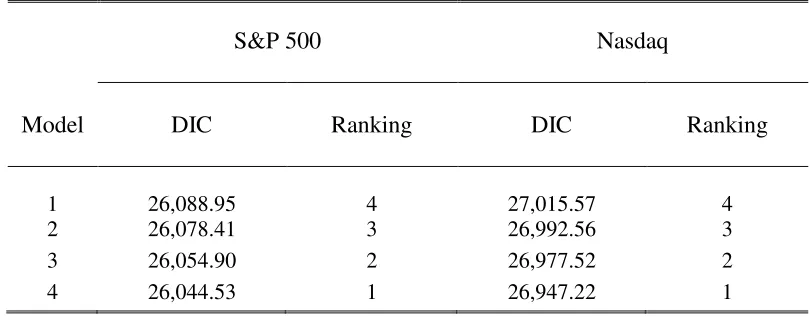
t } for t = 0,1,...,T by running
Algorithm 3-1 (CSMC-AS algorithm).
where X0:t = {x(0:bt0:t), X
(−b0:t)
0:t }; S0:t = {s(0:b0:tt), S
(−b0:t)
PGAS sampler allows a reference trajectory to change its ancestry as we run the conditional SMC
with ancestor sampling in the forward direction. This approach is more robust to path degeneracy
because all the generated particles are fully utilized as in backward simulation to approximate the
joint smoothing distribution of xt and st. As a result, it enables a faster-mixing MCMC kernel
than the benchmark PG sampler.
3.4 Bayesian Model Comparisons: Deviance Information Criterion
Despite of considerable progress in the Bayesian Statistics literature over the last few decades,
Bayesian model comparisons still remain a computationally very difficult task especially when
comparing complex hierarchical models that contains many unknown variables. To resolve this
problem, the Deviance Information Criterion (DIC) was developed as the Bayesian counterpart of
the Akaike information Ceriterion (AIC) by Spiegelhalter et al. (2002). This new model selection
criterion has been gaining more and more popularity allowing applied researchers to enjoy the
benefits of its computational simplicity. To formally carry out Bayesian model comparisons on
completing switching state space models, I adopt DIC which is defined by:
DIC =Eζ|y1:T[−2lnf(y1:T|ζ)] + 2{lnf(y1:T|ζ¯)−Eζ|y1:T[lnf(y1:T|ζ)]} (20)
where y1:T ={y1, y2, ..., yT} represents the entire observation sequence; ζ represents the vector of
the model parameters and the latent variables; and ¯ζ stands for the vector of the posterior means
for ζ. The deviance is defined by D(ζ) =−2lnf(y1:T|ζ) which is frequently used as a measure of
classical model fit. Analogously, the first term of DIC measures Bayesian goodness of fit through
the posterior expectation of the deviance, Eζ|y1:T[−2lnf(y1:T|ζ)]. And the second term of DIC,
2{lnf(y1:T|ζ¯)]−Eζ|y1:T[lnf(y1:T|ζ)]}, is included to impose a penalty on model complexity as in the AIC. This term is called the effective number of parameters and increases as the gap between
the deviance evaluated at ¯ζ and the posterior mean of the deviance gets bigger. A model with a
smaller DIC is more preferred because log likelihood is multiplied by -2.
Once a proposed PG algorithm produces MCMC outputs that are approximately sampled from
First, the calculation of the posterior expectation of the deviance is done though the Monte Carlo
integration as:
Eζ|y1:T[lnf(y1:T|ζ)]≈
1 R
R
X
r=1
lnf(y1:T|ζ(r)),
whereζ(r) stands for the posterior samples atr-th MCMC iteration including the continuous state
xt and the discrete regime state st. Conditional xt and st, evaluating the likelihood function
is trivial. Secondly, we calculate the sample averages of the MCMC samples and evaluate the
deviance at ¯ζ. The effective number of parameters is obtained by simply subtracting 2lnf(y1:T|ζ¯)
by Eζ|y1:T[2lnf(y1:T|ζ)].
3.5 Implementation of Proposed Particle Gibbs Samplers
In practice, the extended target density in equation (14) and associated backwards kernels
can be simplified according to the structure of a particular NLG-SSSM of interest. This section
provides more details on how the suggested PG algorithm is implemented using a specific example.
We consider the regime switching stochastic volatility (RS-SV) model by So et al. (1998):
Regime Switching Stochastic Volatility Model (RS-SV)
yt=µ+exp(
xt−1
2 )ǫt, ǫt ∼i.i.d.N(0,1) (21) xt=δst+φ(xt−1−δst−1) +ut, ut∼i.i.d.N(0, σ
2
u)
where yt is the equity return at timet; xt−1 is the latent log-volatility at timet; and E[ǫtut] = 0.
The current position ofxtis given by a function ofxt−1,st, andst−1 in the transition equation, and
the observation yt is given by a nonlinear function of xt−1 in the measurement equation. Because
xt and yt depend only on a few past states in such a model structure, the forward kernel used in
Algorithm 1-1 is defined by:
pθ(x0:t, s0:t|y1:t) =
fθ(yt|xt−1)gθ(xt|xt−1, st, st−1)gθ(st|st−1) pθ(yt|y1:t−1)
At each time, s(ti) and x(ti) are sequentially generated using the transition probability in equation
(2) and the transition equation in equation (21). Therefore, the important weight at time t in
equation (6) becomes:
ωt(i)∝ fθ(yt|x (i)
t−1)gθ(x(ti)|x
(i)
t−1, s (i)
t , s
(i)
t−1)gθ(s(ti)|s
(i)
t−1) gθ(xt|x(ti−)1, s
(i)
t , s
(i)
t−1)gθ(s(ti)|s
(i)
t−1)
ωt(−i)1
=fθ(yt|x(ti−)1)ω (i)
t−1 ∝ω¯ (i)
t ω
(i)
t−1
(6′)
We obtain the estimate of the importance weight in Algorithm 1-1as:
ˆ
ωt(i)= ω¯ (i)
t ωˆ
(i)
t−1
PN
j=1ω¯ (j)
t ωˆ
(j)
t−1
= fθ(yt|x (i)
t−1)
PN
j=1fθ(yt|x(tj−)1) .
where ˆωt(−i)1 does not affect the weight estimate at all as ˆωt(−i)1 = N1 after the re-sampling step. In
fact, there is no need to evaluate any transition densities in Algorithm 1-1. All we need to run
Algorithm 1-1is to evaluate the likelihood function conditional onx(ti−)1fori= 0,1, ..., T. Once the
preliminary procedure ofAlgorithm 3-2is successfully implemented, we simulate the indexK from
its conditional distribution according to the importance weight at the terminal timeT.
With no exception, the CSMC-AS algorithm in Algorithm 3-1 becomes substantially simple.
The step iii) of Algorithm 3-2 that requires Algorithm 3-1 is run using the backward kernel in
Proposition 2:
Φ(bt−1|θ, X0:t−1, S0:t−1, A0:t−1, x(t:bTt:T), s
(bt:T)
t:T , bt:T)
∝
fθ(yt|xt(−bt−11))gθ(x(tbt)|x
(bt−1)
t−1 , s (bt)
t , s
(bt−1)
t−1 )gθ(s(tbt)|s
(bt−1)
t−1 )
ˆ ω(bt−1)
t−1
∝ω(bt−1)
t−1|T.
(22)
The index variable bt−1 ∈ {1,2, ..., N} is therefore easily drawn with the normalized importance
weight in equation (19). Simulating the remaining model parameters from their conditional
pos-terior distributions are straightforward conditional on the latent states. The model parameters
{µ, δ1, δ2, ..., δK, φ}are drawn from multivariate normal distributions and the remaining parameter
we do not need any Metropolis-Hastings algorithm. The PG samplers explained in this section will
be applied for an empirical illustration in section 4 with slight modifications.
3.6 Performance of Proposed Algorithm: Simulation Study
The main goal of this section is to compare the performance of the proposed PG algorithms
in estimating a NLG-SSSM. For this purpose, I simulate the models in (21) for T = 3000 which
is a typical number of observations for daily stock return data. The model is generated with
{µ = 0, δ1 = −1, δ2 = 0.5, φ = 0.9, σu2 = 0.01, π11 = 0.99, π22 = 0.99} where pjj is the transition
probability for j = 1,2. The selected parameter values are set similar to Bayesian estimates
obtained by actual daily returns. I run the two PG samplers (Algorithm 2-2, Algorithm 3-2) for
comparison. The numbers of particles used in the benchmark PG and the PGAS samplers are
N = 1,000, and N = 20, respectively. I keep the latter 40,000 iterations and discard the initial
1,000 iterations as warm up for all simulations. All Bayesian estimates reported in this section are
the averages of 5 simulations.
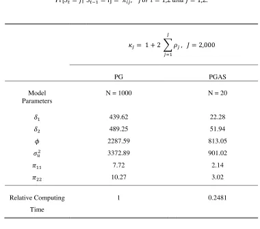
The inefficiency factor developed by Geweke (1992) is one of the popular measures of MCMC
efficiency. The inefficiency factor is computed by autocorrelations in MCMC draws:
κJ = 1 + 2 J
X
j=1 ρj
where ρj represents the autocorrelation for lagj. It is designed to quantify how much inefficiency
loss occurs in calculating posterior moments of a model parameter from serially correlated MCMC
draws. Typically, an MCMC sampler with a high value of the inefficiency factor requires a large
number of posterior simulations to get reliable posterior estimates, which induces high
compu-tational costs. I report Geweke’s (1992) inefficiency factor for selected model parameters of the
RS-SV model. The results in Tables 1 illustrate how much efficiently the proposed PG algorithm
performs in estimating the NLG-SSSM compared to the benchmark algorithm.
The PG sampler with ancestor sampling inAlgorithm 3-2exhibits the best performance
accord-ing to the inefficiency factors reported in Table 1. The inefficiency factors obtained based on the
computing times forAlgorithm 3-2withN = 20 is only 0.2481, compared with the benchmark PG
sampler. Figure 1 shows the autocorrelation functions (ACF) for the model parametersδ1 and φ.
The ACFs very quickly drop to zero with the small numbers of particles when Algorithm 3-2 is
applied. In contrast, the benchmark PG sampler in Algorithm 2-2 does not mix well even with
a large number of particles. It is worth mentioning that the ancestor sampling in Algorithm 3-1
significantly improve the mixing speed without explicitly incorporating the observation sequence
y1:t in the importance distributions of xt and st. In many applications, the proposed PG sampler
can be simplified as explained in the previous section and thus does not impose huge computational
costs. Nevertheless, it reduces the ACFs significantly and achieves faster mixing.
4
Empirical Application: Regime-dependent Leverage Effect of
U.S Stock Market
To illustrate the proposed estimation procedure, I estimate an extended version of the regime
switching stochastic volatility (SV) model by So et al. (1998):
yt=µ+exp(
xt−1
2 )ǫt, (23)
xt=δst +φ(xt−1−δst−1) +ut, (24)
ǫt
ut
∼N(
0
0 ,
1 ρstσu
ρstσu σ2u
)
p(st=j|st−1 =k) =πkj, K
X
j=1
πkj = 1, i, k= 1,2,
where yt is the equity return at time t; xt−1 is the latent log-volatility at timet. We can rewrite
the transition equation in equation (24) as:
xt=δst+φ(xt−1−δst−1) +σu(ρstǫt+ q
1−ρ2
stηt)
=δst+φ(xt−1−δst−1) +σuρstexp(−
xt−1
2 )(yt−µ) +σu q
1−ρ2
stηt
whereηt∼i.i.dN(0,1) andCorr(ǫt, ηt) = 0. According to the above transition equation, it may be
In the literature, the empirical evidence of this negative relationship which is often explained by
leverage effect has been firmly established. Especially, Yu (2005) demonstrated that discrete-time
SV models with the leverage effect are theoretically and empirically appealing in capturing dynamic
interaction between stock return and volatility. The regime switching SV model in equations (23)
and (24) is different from canonical SV models in that it accommodates regime-dependent leverage
effect to take into account a possibility that leverage effect varies over time.
There has been efforts to develop an efficient Bayesian method to estimate a SV model with
leverage. Particularly, Omori et al. (2007) approximated the joint distribution of two correlated
shocks in a SV model with ten mixture normal distributions to transform a SV model with leverage
effect into a partially linear state space model5. However, their approach becomes infeasible when
the correlation parameterρst shifts with unknown timings. Alternatively, one may attempt to use a
single-move algorithm, such as the one adopted by Yu (2012). It is well known that the single-move
approach is difficult to implement with the presence of the very persistent latent regime-indicator
variable, which is often observed in actual data.
Because the existing MCMC algorithms in the literature are not directly applicable in making
Bayesian inference in the proposed SV model, I estimate it by employing the PGAS procedure
discussed in section 3.5. Only slight modifications are made to incorporate the regime switching
correlation parameter ρst. When drawing the variance-covariance matrix of ǫt and ut, I employ
a Metropolis-Hasting algorithm with a candidate multivariate normal distribution. The mean
and covariance matrix of the candidate distribution are found through maximizing the likelihood
function giveny1:T,x0:T,s0:T and a positive definite restriction is imposed on the covariance matrix.
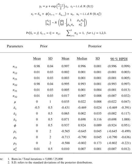
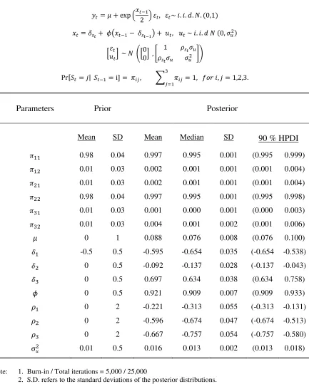
To analyze how the leverage effect changes depending on return volatility, the regime switching
SV model i
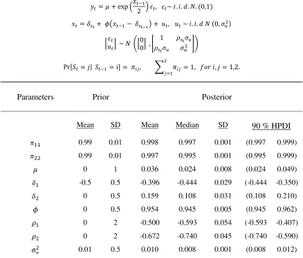
![Table 2.B Bayesian Estimation of SV Model with Regime-dependent Leverage Effect for NASDAQ: 2 State Case [Sample: Jan/02/1975 ~ Aug/05/2015]](https://thumb-us.123doks.com/thumbv2/123dok_us/291853.528745/44.612.87.524.111.483/bayesian-estimation-regime-dependent-leverage-effect-nasdaq-sample.webp)
![Figure 1. Autocorrelation Functions for Selected Model Parameters: Example 1 [T = 3000]](https://thumb-us.123doks.com/thumbv2/123dok_us/291853.528745/48.612.164.460.124.438/figure-autocorrelation-functions-selected-model-parameters-example-t.webp)