Fast Remaining Thickness Measurement Using a Laser Source Scanning Technique

Fast Remaining Thickness Measurement

Using a Laser Source Scanning Technique

Muhammad Nor Salim, Takahiro Hayashi

, Morimasa Murase, Toshihiro Ito and Shoji Kamiya

Graduate School of Engineering, Nagoya Institute of Technology, Nagoya 466-8555, Japan

Fast remaining thickness measurement using Lamb wave is presented for the purpose of maintenance of large structures like oil storage tanks and pipe networks. This study used a laser ultrasonic source to perform a high resolution remote scanning over aluminum plates with grooved and circular defects that were modeled on corrosions in plate-like structures. The antisymmetric A0 and symmetric S0 modes of Lamb wave were used to obtain information of the plate thickness from amplitude distributions over the scanned areas on plates. The amplitude distributions of A0 mode provide better thickness distributions that those of S0 modes for grooved defects. For plates with circular defects, the amplitude distributions did not agree well with the thickness distribution due to the refraction around the defects, defect images were seen in both modes. Especially in the amplitude distribution of S0 mode, the defect images for the circular defect were clearly obtained.

[doi:10.2320/matertrans.I-M2012801]

(Received November 11, 2009; Accepted October 29, 2011; Published February 29, 2012)

Keywords: laser source scanning, Lamb wave, guided wave, ultrasonic

1. Introduction

Guided wave inspection is well known for its ability to perform long range inspection for pipe networks at rapid screening, and low cost inspection. Many studies on pipe and plate inspections have been published by Rose1,2) and co-workers, and Cawley3­5) _{and co-workers who reported} numbers of inspection techniques for plates as well as the inspection techniques for pipes. Many of the guided wave inspections on sites are commonly performed using piezo-electric type transducers,1,3­5) _EMATs,2,6) _and magnetostric-tive sensors7)_{for the excitation and detection on plates and} pipes. Moreover, measurement using laser interferometers8) and pulse laser excitation8­10)_{were also used to increase the} spatial resolution and scanning speed. Although defects can easily be located in the guided wave inspection,1­11) remaining thickness of plates and pipes, the most important factor in maintenances of oil storage tanks and pipe networks, are not evaluated. Therefore, we proposed a laser source scanning over the surface of plates to measure the remaining thickness around the defect region. Remaining thickness of the plates was evaluated from a selected Lamb wave that was excited using an Nd/YAG laser in thermoelastic mode. Generation of ultrasonic wave using a laser source and a galvano laser scanner over plates offers a fast screening with high spatial resolution. This technique also has advantages to perform a remote measurement without elaborative adjustment of the focal length and laser beam direction like the measurement using a laser Doppler vibrometer.11)

The previous study12)discussed the effect of defect depths and shapes of the rounded defect on the transmission coefficient of A0 mode with experimental results. This study investigates the use of S0 mode as well as A0 mode in order to maximize the potential of the technique, and shows the results of circular defects that become frequently a big issue as a corrosion pit in plate like structure, as well as rounded defects.

2. Fundamental Theory

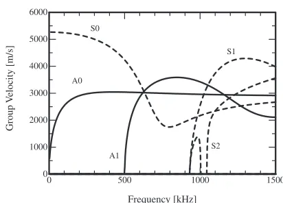
Lamb wave have an advantage over the Rayleigh wave as it may produce stresses throughout plates so that the thickness of the plates could be obtained from the character-istics of the Lamb waves. Moreover, interactions of Lamb wave with defects enable us to locate defects in plate-like structures.4)_{On the contrary, defect inspections using Lamb} wave are complicated because of multiple mode behaviors and dispersions that occur in excitation and measurement of the Lamb wave. Figures 1 and 2, the dispersion curves of Lamb wave modes in an aluminum plate (longitudinal wave velocity CL=6380 m·s¹1 and transverse wave velocity

CT=3080 m·s¹1) with 3 mm thickness, show multi modal behavior and dispersion of Lamb waves in all frequency range. These two characteristics make the application of Lamb waves difficult, because the detected signals may contain many modes with different velocities and the modes may propagate at different velocities with frequency. There-fore, a frequency range with fewer modes and smaller dispersion is widely used to have simple guided wave propagation in the tested structures. In addition, the Lamb wave modes at low frequency below the A1 cut-off frequency

Frequency [kHz]

A0 S0

S1

S2 A1

Group V

elocity

[m/s]

0 500 1000 1500

0 1000 2000 3000 4000 5000 6000

Fig. 1 Group velocity dispersion curves of Lamb wave for an aluminum of 3 mm thickness.

+_{Present address: Toyota Central R&D Labs., INC., Nagakute 480-1192,}

Japan

Special Issue on APCNDT 2009

show a lot of interest as they propagate only in S0 and A0 modes, and a mode selection in guided wave inspection can be made as these modes have different phase velocities below A1 cut-off frequency as shown in Fig. 2.

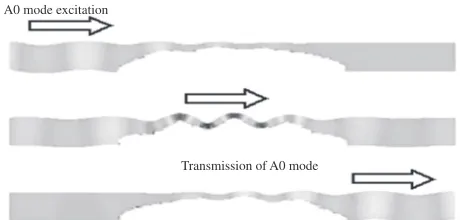
Guided wave propagation in a plate with a rounded shallow defect has been calculated by Hayashi12) using the combination model of semi-analyticalfinite elements (SAFE) and finite element (FE) where the SAFE was used to represent the intact region and the FE was used to model the defect in plate. The result in Fig. 3 shows that the amplitudes of A0 mode introduced from left side of the plate increase as the A0 propagates into the thin region around the defect. The amplitudes of the wave then return to its original amplitudes after propagate completely across the defect. The difference in amplitudes is associated to the difference of thickness in the cross section of the plate that results in different constraints to the propagation of A0 mode in the plate. In other words, in the case where the reflection and mode conversions of the Lamb wave in the vicinity of defects is small, then most of the ultrasonic energy will propagates through the defect. This interaction of the Lamb wave with defect is measurable using a laser interferometer8) that will possibly visualize high amplitudes in the vicinity of the defect.

On the contrary, measurement of the Lamb wave using a laser interferometer in the defect region at high spatial resolution has many disadvantages than generating the Lamb

wave using a pulsed laser. Especially for the applications on curved surfaces of pipes where the focal length and direction of incident beam have to be retained during the scanning process to maintain sensitivity of the measurement. For a solution of the problems, laser source scanning technique and the reciprocal theorem are useful as reported by Takatsubo et al.13) who developed a visualization technique of wave propagation. Using a similar experimental set-up and the reciprocal theorem, amplitude distributions can be obtained as shown in Fig. 4 where signals with higher amplitude are detected on thinner thickness region.

3. Experiments

Experimental system used in the study is shown in Fig. 5 that consists of a Q-switched Nd/YAG pulse laser (Quantel Brilliant Ultra, 532-nm wavelength, 20-Hz rate, 7.2-ns pulse duration, and 32-mJ pulse energy), a laser beam attenuator, a 1-mm slit, and 2-axis galvano laser scanner. Energy of the laser beam was reduced using a laser beam attenuator to avoid damages on the surfaces of galvano mirrors and the test plates. The slit of 1 mm was also used to change the laser spot diameter of 3 mm into a line source of about 3©1 mm2 to improve the spatial resolution of the images. The line source was scanned in the X and Y directions using the 2-axis galvano laser scanner at 161©161 points over scanned areas of 80©80 mm2 _{on test plates. The test plates used in this} study are aluminum plates of 250 mm©150 mm©3 mm with different types of grooved defects and circular defects. Since the characteristics of laser ultrasonic excitations and wave propagations in aluminum plates and pipes are not

A1 S1

0 500 1000 1500

0 1000 2000 3000 4000 5000 6000

Phase V

elocity

[m/s]

Frequency [kHz]

A0

A1 cut-off S0

Fig. 2 Phase velocity dispersion curves of Lamb wave for aluminum of 3 mm thickness.

A0 mode excitation

Transmission of A0 mode

Fig. 3 Propagation of A0 mode around a defect in a plate.“Reprinted with permission from Copyright 2009, Acoustical Society of America (T. Hayashi, M. Murase, and M. Nor Salim, Rapid thickness measurements using guided waves from a scanning laser source, J. Acoust. Soc. Am, Vol. 126, Issue 3, Page 1103).

Low power of laser incidence

Radiation over thin region Radiation over thick region

Plate Defect

Angle beam transducer

Fig. 4 Excitation of A0 modes using laser radiation around a defect in a plate.

500 mm 250 mm

150 mm 3 mm 400 kHz

PZT transducer

2-Axis galvano laser scanner

Scanning area YAG laser 1 mm slit and attenuator

Defect

Y X Wedge

largely different from steel material, which is generally used for large constructions, aluminum plates were used due to their good workability and lightness.

The scanning process was automated using a LabVIEW-based application that sends the signals to the galvano laser scanners to control the position of laser source on plates. A normal beam transducer consisting of a piezoelectric element with central frequency of 400 kHz and aqualene wedge (from Olympus Corp.) were used to measure the A0 mode that propagates from the laser spots at 2300 m·s¹1 of phase velocity. The aqualene was used as a wedge because of its low attenuation of ultrasonic signals and low longitudinal velocity of about 1600 m·s¹1 that allows fabricating the wedge at about 45°.

Though the amplitude distribution of S0 mode has not been proved to show thickness distribution,12)images can be obtained using an angle beam transducer with different beam angle. Measurements were performed with the same 400 kHz transducer and a resin wedge (the longitudinal velocity of 2760 m·s¹1_{, SX-1 from Suzuko Corp.) with about 30° for the} S0 mode.

An analogue low-pass filter of 1 MHz has also been applied to remove the high frequency noise before being amplified by 60 and 64 dB for both A0 and S0 modes, respectively. The signals were then sampled at 5 MHz sampling frequency and filtered using a 400 kHz low-pass filter to extract the component of A0 mode below the cut-off frequency of A1 mode as in Fig. 1. Finally, maximum amplitudes of the signals were used to create an amplitude distribution, which then was converted into thickness distribution in the plates. The laser source was scanned over aluminum plates with grooved and circular defects depicted in Figs. 6 and 7. Figures 6(a) and 6(b) show the grooved defects of 2 and 1 mm depths, respectively. The grooved defects were machined using a ball end mill (diameter 20 mm) and has a flat zone 10 mm at the bottom of each defect. Figures 7(a) and 7(b) show the 2 mm depth of a circular defect and 4 circular defects, respectively. The circular defects were machined using a corner radius end mill (cutter diameter 32 mm and corner radius 10 mm) and have a defect-mouth of diameter 24 mm at the top with circularflat zone of diameter 12 mm at the bottom in each circular defect.

4. Results and Discussions

4.1 Conversion into thickness distributions

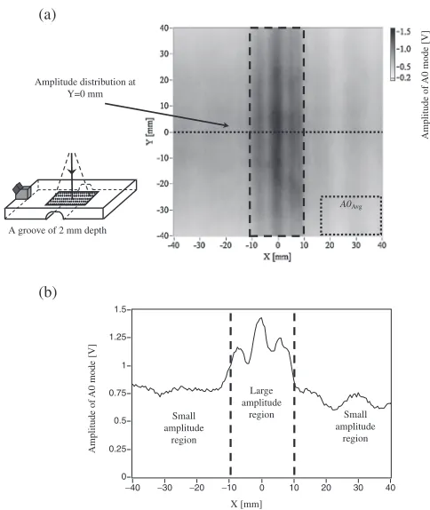
Figure 8 shows amplitude distributions for the plate with 2 mm depth grooved defect using the angle beam transducer for A0 mode at X=¹200 mm and Y=0 mm. (a) is the distribution of the scanning area fromX=¹40 to+40 and

from Y=¹40 to +40 representing the amplitude in grayscale from 0 to 1.5 V, and (b) is the distribution on the center line at Y=0 mm. These figures show that the amplitude distributions of A0 mode below the cut-off frequency of A1 mode are roughly inverse proportional to the thickness distributions as presented in the previous study.12)_{Then, the remaining thickness can be obtained by}

tA0ðX; YÞ ¼ Aavg

AðX; YÞd ð1Þ

(a) (b)

10 mm

22 mm

2 mm

3 mm 150 mm

10 mm

18 mm

1 mm

3 mm 150 mm

Fig. 6 Configuration of grooved defects: (a) A grooved defect with 2 mm maximum depth and (b) 1 mm maximum depth.

(a)

(b)

3 mm

24 mm 12 mm

40 mm

150 mm 40 mm

12 mm 24 mm

2 mm

3 mm 75 mm

Fig. 7 Configuration of circular defects with 2 mm maximum depth: (a) A circular defect and (b) four circular defects.

(a)

(b) A groove of 2 mm depth

Amplitude of

A0 mode [V]

Amplitude distribution at Y=0 mm

A0Avg

Amplitude of

A0 mode

[V]

1.5

0 0.25 0.5 0.75 1 1.25

40

−40 −30 −20 −10 0 10 20 30

Large amplitude

region Small

amplitude region

Small amplitude

region

X [mm]

where Aavg, AðX; YÞ, and d are the average of A0 mode

amplitudes in a intact region, amplitude of A0 mode at (X,Y), and original thickness over intact region, respectively. In this study, the amplitudes at a selected intact region are averaged forAavg.

Similarly the remaining thickness in plate for using S0 mode,tS0ðX; YÞcan be roughly evaluated from the amplitude distribution by

tS0ðX; YÞ ¼ Savg

SðX; YÞd ð2Þ

where Savg, SðX; YÞ, and d are the average of S0 mode amplitudes in a selected intact region, amplitude of S0 mode at (X,Y), and original thickness over the intact region, respectively.

The amplitudes distributions over defects in the experi-ments were converted into the thickness distributions for A0 and S0 modes using the eqs. (1) and (2), respectively.

4.2 Thickness distributions

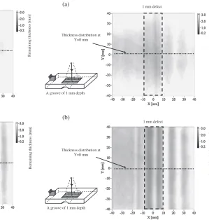
Figures 9 and 10 show the thickness distributions for the plates with grooved defects with the maximum depths of 1 and 2 mm, respectively. (a) and (b) are for the measurements of A0 and S0 modes, respectively. Figures 9(a) and 10(a) show the same results in the previous study,12) where the thickness distributions can be roughly obtained using A0 mode below the cut-off frequency of A1 mode. Rough thickness distributions were also observed even for S0 mode in Figs. 9(b) and 10(b). In the Figs. 9(b) and 10(b), striped patterns caused by reflection and low transmission ratio of S0

mode at the defects can be seen in the intact areas at the both sides of the defects. Besides, large oscillation of the distribution changes can also be seen in the defect region, which is caused by the multiple reflections in the defect region.

The thickness distributions can be clearly seen in Figs. 11 and 12, where the remaining thickness calculated by eqs. (1) and (2) at Y=0 mm are plotted. Figures 11(a) and 12(a) correspond to the amplitude changes at the centerline of Figs. 9(a) and 10(a) for A0 mode. The remaining thickness was indicated at about 1.4 mm for the 2 mm grooved defect and at about 2.1 mm for the 1 mm grooved defect. On the other hand, Figs. 11(b) and 12(b) correspond to the amplitude changes at the centerline of Figs. 9(b) and 10(b) for S0 mode. The 2 mm grooved defect shows the remaining thickness at about 1.2 mm in Fig. 11(b), and 1 mm grooved defect shows the remaining thickness at about 1.8 mm in Fig. 12(b). Comparing the conventional point-by-point testing using an ultrasonic thickness gage, this technique may be inaccurate, but for a rapid screening inspection, these results are useful to find defects and roughly evaluate the remaining thickness especially using A0 mode.

Figures 13 and 14 show the thickness distributions for the test plates with circular defects. The result from a circular defect of 2 mm maximum depth is shown in Fig. 13, while the result over the four circular defects with the same maximum depth is shown in Fig. 14. The changes of thickness level in Y direction at X=0 mm (center of the single circular defect) andX=¹20 mm (center of the front (b)

A groove of 2 mm depth Thickness distribution at

Y=0 mm

Remaining thickness [mm]

2 mm defect (a)

A groove of 2 mm depth Thickness distribution at

Y=0 mm

Remaining thickness [mm]

2 mm defect

Fig. 9 Thickness distributions on plate with a grooved defect of 2 mm maximum depth: (a) Evaluated from A0 and (b) S0 modes.

(a)

(b)

Thickness distribution at Y=0 mm

Remaining thickness [mm]

1 mm defect

A groove of 1 mm depth A groove of 1 mm depth

Thickness distribution at Y=0 mm

Remaining thickness [mm]

1 mm defect

(a)

(b)

3

0 0.5 1 1.5 2 2.5

40

−40 −30 −20 −10 0 10 20 30

Thickness of S0 mode [mm]

Defect region

Intact region Intact region

X [mm] Large oscillation

3

0 0.5 1 1.5 2 2.5

40

−40 −30 −20 −10 0 10 20 30

Thickness of

A0 mode [mm]

Defect region

Intact region Intact region

X [mm]

Fig. 11 Thickness distribution atY=0 mm on plate with a grooved defect of 2 mm maximum depth: (a) A0 mode thickness distribution and (b) S0 mode thickness distribution.

(b)

3

0 0.5 1 1.5 2 2.5

40

−40 −30 −20 −10 0 10 20 30

Thickness of S0 mode [mm]

Defect region

Intact region Intact region

X [mm] Large oscillation

(a)

3

0 0.5 1 1.5 2 2.5

40

−40 −30 −20 −10 0 10 20 30

Thickness of

A0 mode [mm]

Defect region

Intact region Intact region

X [mm]

Fig. 12 Thickness distribution atY=0 mm on plate with a grooved defect of 1 mm maximum depth: (a) A0 mode thickness distribution and (b) S0 mode thickness distribution.

(a)

(b)

A circular defect of 2 mm depth Thickness distribution at

X=0 mm

Remaining thickness [mm]

2 mm circular defect

Bottom edge

Top edge A circular defect of 2 mm depth

Thickness distribution at X=0 mm

Remaining thickness [mm]

2 mm circular defect

Bottom edge

Top edge

Fig. 13 Thickness distributions on plate with a circular defect of 2 mm maximum depth: (a) Evaluated from A0 and (b) S0 modes.

(a)

(b)

Thickness distribution at X= -20 mm

Remaining thickness [mm]

2 mm circular defects

Bottom edge

Top edge Four circular defects of 2 mm depth

Thickness distribution at X= -20 mm

Remainin

g

thickness [mm]

2 mm circular defects

Bottom edge

Top edge

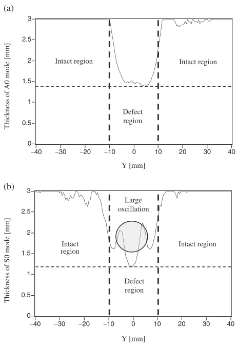
defects in the plate with multiple circular defects) are also shown in Figs. 15 and 16, which correspond to the thickness profile in Fig. 7. From Figs. 15(a) and 16(a) the remaining thickness over the circular defect with 2 mm maximum depth was also evaluated from A0 mode about 1.2 mm thickness. However, only the first two defects facing to the transducer were evaluated in Fig. 14(a), and the rest two defects behind the front ones were not been evaluated properly. This is due to the complicated refractions of Lamb wave around the defects and indicates difficulties in thickness measurement using this technique in this situation. Similar to the previous defects, the thickness distributions from the measurement of S0 mode in Figs. 13(b) and 14(b) shows clearer shape of the circular defects in plates but they appeared with non-uniform stripes that indicated large oscillations in the profile of the thickness as in Figs. 15(b) and 16(b).

5. Conclusions

A study of thickness evaluation in plates was conducted using a laser source scanning technique and an angle beam transducer. Amplitudes of the excited A0 and S0 modes show large amplitudes over the region with a small remaining thickness and small amplitudes over the large remaining thickness in a low frequency range. The mode then were converted into thickness distributions and used to character-ize remaining thickness in plates with grooved and circular

defects. The grooved defects were used to demonstrate the results in plates with simple defect shape that have less boundary surfaces while the circular defects were used to demonstrate results in plates that close to the shape of corrosion and pitting defects found in actual pipe. Both modes indicated thickness loss over the defects in plate but show some differences in sensitivity.

From the experiment, we concluded that the amplitude distributions using the A0 mode shows a great potential for the estimation of remaining thickness over defects in plates. In contrast, the results from S0 mode are probably useful to identify the shape of the defects. However, both show potential of such a nondestructive testing method to characterize defects and evaluate the remaining thickness of plates and pipes, which is usually the most important factor in maintenances of oil storage tanks and pipe networks that are not evaluated in typical guided wave inspection techniques.

REFERENCES

1) J. L. Rose, S. P. Pelts and M. J. Quarry:Ultrasonics36(1998) 163­169.

2) W. Luo, X. Zhao and J. L. Rose: Review of Progress in QNDE24A, ed. by D. O. Thompson and D. E. Chimenti, (American Institute of Physics, Melville, NY, 2005) pp. 105­111.

3) M. J. S. Lowe, D. N. Alleyne and P. Cawley:Ultrasonics36(1998)

147­154.

4) P. Cawley and D. N. Alleyne:Ultrasonics34(1996) 287­290.

5) D. N. Alleyne and P. Cawley: Mater. Eval.55(1997) 504­508. (a)

(b) ₃

0 0.5 1 1.5 2 2.5

40

−40 −30 −20 −10 0 10 20 30

Thickness of S0 mode [mm]

Defect region Intact

region

Y [mm]

Intact region Large

oscillation

3

0 0.5 1 1.5 2 2.5

40

−40 −30 −20 −10 0 10 20 30

Thickness of

A0

mode [mm]

Intact region

Y [mm]

Intact region

Defect region

Fig. 15 Thickness distribution atX=0 mm on plate with a circular defect of 2 mm maximum depth: (a) A0 mode thickness distribution and (b) S0 mode thickness distribution.

(a)

(b) 3

0 0.5 1 1.5 2 2.5

40

−40 −30 −20 −10 0 10 20 30

Thickness of S0 mode [mm]

Defect region Intact

region

Y [mm]

Intact region Large

oscillation

Intact region

Defect region

3

0 0.5 1 1.5 2 2.5

40

−40 −30 −20 −10 0 10 20 30

Thickness of

A0 mode [mm]

Intact region

Y [mm]

Intact region

Defect region Defect

region

Intact region

6) M. Hirao and H. Ogi:Ultrasonics35(1997) 413­421.

7) H. Kwun and S. Y. Kim:J. Pressure Vessel Technol.127(2005) 284­ 289.

8) C. B. Scruby and L. E. Drain: Laser Ultrasonics Techniques and Applications, (Adam Hilger, Bristol, England, 1990).

9) S. S. Lee, Y. G. Kim, B. Y. Ahn and S. W. Dho: Review of Progress in QNDE20A, ed. by D. O. Thompson and D. E. Chimenti, (American Institute of Physics, Melville, NY, 2001) pp. 97­104.

10) A. K. Kromine, P. A. Fomitchov, S. Krishnaswamy and J. D. Achenbach: Review of Progress in QNDE 20B, ed. by D. O.

Thompson and D. E. Chimenti, (American Institute of Physics, Melville, NY, 2001) pp. 1612­1617.

11) T. Hayashi, Y. Kojika, K. Kataoka and M. Takikawa: Review of progress in QNDE27A, ed. by D. O. Thompson and D. E. Chimenti, (American Institute of Physics, Melville, NY, 2007) pp. 178­184. 12) T. Hayashi, M. Murase and M. Nor Salim:J. Acoust. Soc. Am126

(2009) 1101­1106.

13) J. Takatsubo, B. Wang, H. Tsuda and N. Tooyama:J. Solid Mech.