Density Maximization in Context Sense Metric Space for All words WSD

Density Maximization in Context-Sense Metric Space

for All-words WSD

Koichi Tanigaki†‡ _{Mitsuteru Shiba}† _{Tatsuji Munaka}† _{Yoshinori Sagisaka}‡

†Information Technology R&D Center, Mitsubishi Electric Corporation 5-1-1 Ofuna, Kamakura, Kanagawa 247-8501, Japan

‡Global Information and Telecommunication Institute, Waseda University 1-3-10 Nishi-Waseda, Shinjuku-ku, Tokyo 169-0051, Japan

Abstract

This paper proposes a novel smoothing model with a combinatorial optimization scheme for all-words word sense disam-biguation from untagged corpora. By gen-eralizing discrete senses to a continuum, we introduce a smoothing in context-sense space to cope with data-sparsity result-ing from a large variety of lresult-inguistic con-text and sense, as well as to exploit sense-interdependencyamong the words in the same text string. Through the smoothing, all the optimal senses are obtained at one time under maximum marginal likelihood criterion, by competitive probabilistic ker-nels made to reinforce one another among nearby words, and to suppress conflicting sense hypotheses within the same word. Experimental results confirmed the superi-ority of the proposed method over conven-tional ones by showing the better perfor-mances beyond most-frequent-sense base-line performance where none of SemEval-2 unsupervised systems reached.

1 Introduction

Word Sense Disambiguation (WSD) is a task to identify the intended sense of a word based on its context. All-words WSD is its variant, where all the unrestricted running words in text are expected to be disambiguated. In the all-words task, all the senses in a dictionary are potentially the target destination of classification, and purely supervised approaches inherently suffer from data-sparsity problem. The all-words task is also character-ized bysense-interdependencyof target words. As the target words are typically taken from the same

text string, they are naturally expected to be inter-related. Disambiguation of a word should affect other words as an important clue.

From such characteristics of the task, knowledge-based unsupervised approaches have been extensively studied. They compute dictionary-based sense similarity to find the most related senses among the words within a certain range of text. (For reviews, see (Agirre and Edmonds, 2006; Navigli, 2009).) In recent years, graph-based methods have attracted considerable attentions (Mihalcea, 2005; Navigli and Lapata, 2007; Agirre and Soroa, 2009). On the graph structure of lexical knowledge base (LKB), random-walk or other well-known graph-based techniques have been applied to find mutually related senses among target words. Unlike earlier studies disambiguating word-by-word, the graph-based methods obtainsense-interdependent solution for target words. However, those methods mainly focus on modeling sense dis-tribution and have less attention to contextual smoothing/generalization beyond immediate context.

There exist several studies that enrich immedi-ate context with large corpus statistics. McCarthy et al. (2004) proposed a method to combine sense similarity with distributional similarity and config-ured predominant sense score. Distributional sim-ilarity was used to weight the influence of context words, based on large-scale statistics. The method achieved successful WSD accuracy. Agirre et al. (2009) used a k-nearest words on distributional similarity as context words. They apply a LKB graph-based WSD to a target word together with the distributional context words, and showed that it yields better results on a domain dataset than just using immediate context words. Though these

studies are word-by-word WSD for target words, they demonstrated the effectiveness to enrich im-mediate context by corpus statistics.

This paper proposes asmoothing modelthat in-tegrates dictionary-based semantic similarity and corpus-based context statistics, where a combina-torial optimization scheme is employed to deal with sense interdependency of the all-words WSD task. The rest of this paper is structured as fol-lows. We first describe our smoothing model in the following section. The combinatorial optimization method with the model is described in Section 3. Section 4 describes a specific implementation for evaluation. The evaluation is performed with the SemEval-2 English all-words dataset. We present the performance in Section 5. In Section 6 we dis-cuss whether the intended context-to-sense map-ping and the sense-interdependency are properly modeled. Finally we review related studies in Sec-tion 7 and conclude in SecSec-tion 8.

2 Smoothing Model

Let us introduce in this section the basic idea for modeling context-to-sense mapping. The distance (or similarity) metrics are assumed to be given for context and for sense. A specific implementation of these metrics is described later in this paper, for now the context metric is generalized with a dis-tance function dx(·,·) and the sense metric with

ds(·,·). Actually these functions may be arbitrary

ones that accept two elements and return a positive real number.

Now suppose we are given a dataset concern-ing N number of target words. This dataset is denoted byX = {xi}N_i=1, wherexi corresponds

to the context of the i-th word but not the word by itself. For each xi, the intended sense of the

word is to be found in a set of sense candidates Si = {sij}Mj=1i ⊆ S, whereMi is the number of

sense candidates for thei-th word,S is the whole set of sense inventories in a dictionary. Let the two-tuple hij = (xi, sij) be the hypothesis that

the intended sense inxi issij. The hypothesis is

an element of the direct productH =X×S. As

(X, dx)and(S, ds)each composes a metric space,

H is also a metric space, provided a proper dis-tance definition withdxandds.

Here, we treat the spaceHas a continuous one, which means that we assumethe relationship be-tween context and sense can be generalized in con-tinuous fashion. In natural language processing,

continuity has been sometimes assumed for lin-guistic phenomena including word context for cor-pus based WSD. As for classes or senses, it may not be a common assumption. However, when the classes for all-words WSD are enormous, fine-grained, and can be associated with distance, we can rather naturally assume the continuity also for senses. According to the nature of continuity, once given a hypothesishij for a certain word, we can

extrapolate the hypothesis for another word of an-other sensehi′_j′ = (x_i′, s_i′_j′)sufficiently close to

hij. Using a Gaussian kernel (Parzen, 1962) as a

smoothing model, the probability density extrapo-lated athi′_j′ givenhij is defined by their distance

as follows:

K(hij, hi′_j′) (1)

≡ 1

2πσxσs

exp

[

−dx 2_(x

i, xi′)

2σx2 −

ds2(sij, si′j′)

2σs2

]

,

where σx and σs are parameters of positive real

number σx, σs ∈ R+ called kernel bandwidths.

They control the smoothing intensity in context and in sense, respectively.

Our objective is to determine the optimal sense for all the target words simultaneously. It is es-sentially a 0-1 integer programing problem, and is not computationally tractable. We relax the integer constraints by introducing a sense prob-ability parameter πij corresponding to each hij.

πij denotes the probability by which hij is true.

As πij is a probability, it satisfies the constraints ∀i ∑_jπij = 1and∀i, j0≤πij ≤1. The

proba-bility density extrapolated athi′_j′ by a

probabilis-tichypothesishij is given as follows:

Qij(hi′_j′) ∝ π_ijK(h_ij, h_i′_j′). (2)

decoy

flora H.B. Tree(actor)

tree diagram tree

Sense Probability

Hypothesis

Context Metric Space Context (Input)

Sense Metric

Space _Extrapolated

Density

Sense (Class)

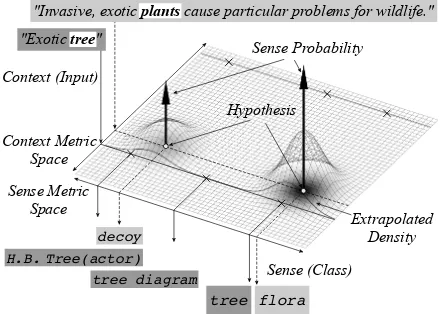
"Invasive, exotic plants cause particular problems for wildlife." "Exotic tree"

Figure 1: Proposed probability distribution model for context-to-sense mapping space.

what context. The upward arrow on a hypothesis represents the magnitude of its probability.

Centered on each hypotheses, a Gaussian ker-nel is placed as a smoothing model. It extrapo-lates the hypotheses of other words around it. In accordance with geometric intuition, intensity of extrapolation is affected by the distance from a hy-pothesis, and by the probability of the hypothesis by itself. Extrapolated probability density is rep-resented by shadow thickness and surface height. If there is another word in nearby context, the ker-nels can validate the sense of that word. In the figure, there are two kernels in the context “Inva-sive, exotic ...”. They are two competing hypothe-sis for the sensesdecoyandfloraof the word plants. These kernels affect the senses of another ambiguous word tree in nearby context “Exotic ...”, and extrapolate the most at the sense tree nearbyflora. The extrapolation has non-linear effect. It affects little to the word far away in con-text or in sense as is the case for the background word in the figure. Strength of smoothing is deter-mined by kernel bandwidths. Wider bandwidths bring stronger effect of generalization to further hypotheses, but too wide bandwidths smooth out detailed structure. The bandwidths are the key for disambiguation, therefore they are to be optimized on a dataset together with sense probabilities.

3 Simultaneous Optimization of All-words WSD

Given the smoothing model to extrapolate the senses of other words, we now make its in-stances interact to obtain the optimal combination of senses for all the words.

3.1 Likelihood Definition

Let us first define the likelihood of model param-eters for a given dataset. The paramparam-eters con-sist of a context bandwidthσx, a sense bandwidth

σs, and sense probabilities πij for all i and j.

For convenience of description, the sense proba-bilities are all together denoted as a vector π = (. . . , πij, . . .)⊤, in which actual order is not the

matter.

Now remind that our dataset X = _{x_i}N i=1 is

composed ofN instances ofunlabeledword con-text. We consider all the mappings from context to sense are latent, and find the optimal parameters by maximizing marginal pseudo likelihood based on probability density. The likelihood is defined as follows:

L(π, σx, σs;X) ≡ ln

∏

i

∑

j

πijQ(hij), (3)

where∏_i denotes the product overxi ∈ X,∑_j

denotes the summation over all possible senses sij ∈ Si for the current i-th context. Q(hij)

denotes the probability density at hij. We

com-pute Q(hij)using leave-one-out cross-validation

(LOOCV), so as to prevent kernels from over-fitting to themselves, as follows:

Q(hij) (4)

≡ _N 1

−Ni

∑

i′_:wi′̸=wi

∑

j′

πi′j′K(hij, hi′j′),

whereNidenotes the number of occurrences of a

word type wi in X, and ∑_i′_:w

i′̸=wi denotes the summation overxi′ ∈ Xexcept the case that the

word typewi′ equals towi.∑j′ denotes the

sum-mation over si′_j′ ∈ S_i′. We take as the unit of

LOOCV not a word instance but a word type, be-cause the instances of the same word type invari-ably have the same sense candidates, which still cause over-fitting when optimizing the sense band-width.

3.2 Parameter Optimization

We are now ready to calculate the optimal senses. The optimal parametersπ∗, σ∗_x, σ_s∗are obtained by maximizing the likelihood L subject to the con-straints onπ, that is_∀i∑_jπij = 11. Using the

Lagrange multipliers {λi}N

i=1 for every i-th

con-straint, the solution for the constrained

maximiza-1_{It is guaranteed that the other constraints}

∀i, j0_≤πij_≤

tion ofLis obtained as the solution for the equiv-alent unconstrained maximization of_Lˇ_{as follows:}

π∗, σ∗_x, σ_s∗ = arg max

π, σx, σs

ˇ

L, (5)

where

ˇ

L ≡ L+∑

i

λi

( ∑

j

πij−1

)

. (6)

When we optimize the parameters, the first term of Equation (6) in the right-hand side actsto re-inforcenearby hypotheses among different words, whereas the second term actsto suppress conflict-ing hypotheses of the same word.

Taking ∇Lˇ = 0, erasing λi, and rearranging,

we obtain the optimal parameters as follows:

πij =

∑

i′, j′

wi′ ̸=_wi Riij′_j′ +

∑

i′, j′

wi′ ̸=_wi Riji′j′

1 + ∑_j∑_i′, j′

wi′ ̸=_wi Riji′j′

(7)

σx2 =

1

N

∑

i, i′_{, j, j}′

wi′ ̸=_wi

Riij′_j′dx2(xi, xi′) (8)

σs2 =

1

N

∑

i, i′, j, j′

wi′ ̸=_wi

Riij′_j′ds2(sij, si′j′), (9)

where Riij′j′ denotes the responsibility of hi′_j′ to

hij: the ratio of total expected density athij, taken

up by the expected density extrapolated by hi′j′,

normalized to the total forxibe1. It is defined as

Riij′j′ ≡

πijQi′j′(hij)

∑

jπijQ(hij)

. (10)

Qi′_j′(h_ij) denotes the probability density at h_ij

extrapolated byhi′j′ alone, defined as follows:

Qi′_j′(hij) ≡

1

N −Ni

π_i′_j′K(hij, hi′_j′). (11)

Intuitively, Equations (7)-(9) are interpreted as follows. As for Equation (7), the right-hand side of the equation can be divided as the left term and the right term both in the numerator and in the denominator. The left term requires πij to agree

with the ratio of responsibilityof the whole tohij.

The right term requiresπij to agree with the

ra-tio of responsibility of hij to the whole. As for

Equation (8), (9), the optimal solution is the mean squared distance in context, and in sense, weighted by responsibility.

To obtain the actual values of the optimal pa-rameters, EM algorithm (Dempster et al., 1977) is applied. This is because Equations (7)-(9) are circular definitions, which include the objective parameters implicitly in the right hand side, thus the solution is not obtained analytically. EM al-gorithm is an iterative method for finding maxi-mum likelihood estimates of parameters in statis-tical models, where the model depends on unob-served latent variables. Applying the EM algo-rithm to our model, we obtain the following steps:

Step 1. Initialization: Set initial values to π, σx, and σs. As for sense probabilities,

we set the uniform probability in accor-dance with the number of sense candidates, thereby πij ← |Si|−1, where |Si| denotes

the size of Si. As for bandwidths, we set

the mean squared distance in each metric; thereby σx2 ← N−1∑_{i, i}′dx2(xi, xi′)

for context bandwidth, and σs2 ←

(∑_i|S_i|)−1∑_{i, i}′∑j, j′ds2(sij, si′j′) for

sense bandwidth.

Step 2. Expectation: Using the current parame-tersπ,σx, andσs, calculate the

responsibili-tiesRiij′_j′ according to Equation (10).

Step 3. Maximization: Using the current respon-sibility Riij′j′, update the parameters π, σx,

andσs, according to Equation (7)-(9). Step 4. Convergence test: Compute the

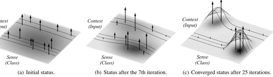
likeli-hood. If its ratio to the previous iteration is sufficiently small, or predetermined number of iterations has been reached, then terminate the iteration. Otherwise go back to Step 2. To visualize how it works, we applied the above EM algorithm to pseudo 2-dimensional data. The results are shown in Figure 2. It simulates WSD for anN = 5words dataset, whose contexts are

Context (Input)

Sense (Class)

(a) Initial status.

Context (Input)

Sense (Class)

(b) Status after the 7th iteration.

Context (Input)

Sense (Class)

(c) Converged status after 25 iterations.

Figure 2: Pseudo 2D data simulation to visualize the dynamics of the proposed simultaneous all-words WSD with ambiguous five words and twelve sense hypotheses. (There are twelve Gaussian kernels at the base of each arrow, though the figure shows just their composite distribution. Those kernels reinforce and compete one another while being fitted their affecting range, and finally settle down to the most consistent interpretation for the words with appropriate generalization. For the dynamics with an actual dataset, see Figure 5.)

which is rather broad and makes kernels strongly smoothed, thus the model captures general struc-ture of space. Figure 2(b) shows the status after the 7th iteration. Bandwidths are shrinking especially in context, and two context clusters, so to speak, two usages, are found. Figure 2(c) shows the sta-tus of convergence after 25 iterations. All the ar-row lengths incline to either 1 or 0 along with their neighbors, thus all the five words are now disam-biguated.

Note that this is not the conventional cluster-ing of observed data. If, for instance, the Gaus-sian mixture clustering of 2-mixtures is applied

to the positions of these hypotheses, it will find the clusters just like Figure 2(b) and will stop. The cluster centers are located at the means of hy-potheses including miscellaneous alternatives not intended, thus the estimated probability distribu-tion is, roughly speaking, offset toward the center of WordNet, which is not what we want. In con-trast, the proposed method proceeds to Figure 2(c) and finds clustersin the data after conflicting data is erased. This is because our method is aim-ing at modelaim-ing not the disambiguation of cluster-memberships but the disambiguation of senses for each word.

4 Metric Space Implementation

So far, we have dealt with general metrics for con-text and for sense. This section describes a spe-cific implementation of those metrics employed in the evaluation. We followed the previous study by McCarthy et al. (2004), (2007), and imple-mented a type-based WSD. The context of word

instances are tied to the distributional context of the word type in a large corpus. To calculate sense similarities, we used the WordNet similarity pack-age by Pedersen et al. (2004), version 2.05. Two measures proposed by Jiang and Conrath (1997) and Lesk (1986) were examined, which performed best in the previous study (McCarthy et al., 2004).

Distributional similarity (Lin, 1998) was computed among target words, based on the statistics of the test set and the background text provided as the official dataset of the SemEval-2 English all-words task (Agirre et al., 2010). Those texts were parsed using RASP parser (Briscoe et al., 2006) version 3.1, to obtain grammatical relations for the distributional similarity, as well as to obtain lemmata and part-of-speech (POS) tags which are required to look up the sense inventory of WordNet. Based on the distributional similarity, we just usedk-nearest neighbor words as the context of each target word. Although it is an approximation, we can expect reliability im-provement often seen by ignoring the lower part. In addition, this limitation of interactions highly reduces computational cost in particular when applying to larger-scale problems. To do this, the exhaustive sum ∑_{i, i}′:wi̸=wi′ in Equation (7)-(9) is altered by the local sum ∑_{i, i}′: (wi,wi′)∈PkNN,

where PkNN denotes the set of word pairs of

which either is a k-nearest neighbors of the other. The normalizing factors1,N, andN₋Ni

in Equation (7), (8)-(9), and (11) are altered by the actual sum of responsibilities within those neighbors as ∑_i′_{, j, j}′_{: (wi,wi′)∈P}

∑

i, i′_{, j, j}′_{: (wi,wi′)∈P}

kNNR ij

i′j′, and

∑

ι, i′_{, j, j}′_{: (wι,w}

i′)∈PkNN∧ι̸=iR ιj

i′j′, respectively.

To treat the above similarity functions of con-text and of sense as distance functions, we use the conversion: d(_·,_·) _{≡ −}αln(f(_·,_·)/fmax), where

ddenotes the objective distance function, i.e.,dx

for context anddsfor sense, whilef andfmax

de-note the original similarity function and its max-imum, respectively. α is a standardization co-efficient, which is determined so that the mean squared distance be1 in a dataset. According to

this standardization, initial values ofσx2,σs2 are

always1.

5 Evaluation

To confirm the effect of the proposed smoothing model and its combinatorial optimization scheme, we conducted WSD evaluations. The primary evaluations compare our method with conven-tional ones, in Section 5.2. Supplementary eval-uations are described in the subsequent sections that include the comparison with SemEval-2 par-ticipating systems, and the analysis of model dy-namics with the experimental data.

5.1 Evaluation Scheme

To make the evaluation comparable to state-of-the-art systems, we used the official dataset of the SemEval-2 English all-words WSD task (Agirre et al., 2010), which is currently the latest pub-lic dataset available with published results. The dataset consists of test data and background doc-uments of the same environment domain. The test data consists of 1,398 target words (1,032 nouns and 366 verbs) in 5.3K running words. The background documents consists of 2.7M running words, which was used to compute distributional similarity.

Precisions and recalls were all computed us-ing the official evaluation tool scorer2in fine-grained measure. The tool accepts answers either in probabilistic format (senses with probabilities for each target word) or in deterministic format (most likely senses, with no score information). As the proposed method is a probability model, we evaluated in the probabilistic way unless explicitly noted otherwise. For this reason, we evaluated all the sense probabilities as they were. Disambigua-tions were executed in separate runs for nouns and verbs, because no interaction takes place across POS in this metric implementation. The two runs’

results were combined later to a single answer to be input toscorer2.

The context metric space was composed by k -nearest neighbor words of distributional similarity (Lin, 1998), as is described in Section 4. The value ofkwas evaluated for_{2, 3, 5, 10, 20, 30, 50, 100, 200, 300}. As for sense metric space, we evalu-ated two measures i.e., (Jiang and Conrath, 1997) denoted asJCN, and (Lesk, 1986) denoted asLesk. In every condition, stopping criterion of iteration is always the number of iteration (500 times), irre-spective of the convergence in likelihood.

Primary evaluations compared our method with two conventional methods. Those methods differ to ours only in scoring schemes. The first one is the method by McCarthy et al. (2004), which determines the word sense based on sense simi-larity and distributional simisimi-larity to thek-nearest neighbor words of a target word by distributional similarity. Our major advantage is the combina-torial optimization framework, while the conven-tional one employs word-by-word scheme. The second one is based on the method by Patwardhan et al. (2007), which determines the word sense by maximizing the sum of sense similarity to the k immediate neighbor words of a target word. Thek words were forced to be selected from other target words of the same POS to the word of interest, so as to make information resource equivalent to the other comparable two methods. It is also a word-by-word method. It exploits no distributional simi-larity. Our major advantages are the combinatorial optimization scheme and the smoothing model to integrate distributional similarity. In the following section, these comparative methods are referred to asMc2004andPat2007, respectively.

5.2 Comparison with Conventional Methods

Let us first confirm our advantages compared to the conventional methods of Mc2004 and Pat2007. The comparative results are shown in Figure 3 in recall measure. Precisions are simply omitted be-cause the difference to the recalls are always the number of failures on referring to WordNet by mislabeling of lemmata or POSs, which is always the same for the three methods. Vertical range de-picts 95% confidence intervals. The graphs also indicate the most-frequent-sense (MFS) baseline estimated from out-of-domain corpora, whose re-call is 0.505 (Agirre et al., 2010).

Contextk-NN Contextk-NN 0.4

0.5

1 10 100 1000

0.4 0.5

1 10 100 1000

MFS

Re

ca

ll

(a) JCN (b) Lesk

Re

ca

ll

MFS Proposed

Mc2004

Pat2007

Proposed

Mc2004

Pat2007

Figure 3: Comparison to the conventional methods that differ to our method only in scoring schemes.

Table 1: Comparison with the top-5 knowledge-based systems in SemEval-2 (JCN/k= 5).

Rank Participants R P Rn Rv

- Proposed (best) 50.8 51.0 52.5 46.2 - MFS Baseline 50.5 50.5 52.7 44.3 1 Kulkarni et al. (2010) 49.5 51.2 51.6 43.4 2 Tran et al. (2010) 49.3 50.6 51.6 42.6 3 Tran et al. (2010) 49.1 50.4 51.5 42.5 4 Soroa et al. (2010) 48.1 48.1 48.7 46.2 5 Tran et al. (2010) 47.9 49.2 49.4 43.4

... ... ... ... ... ...

- Random Baseline 23.2 23.2 25.3 17.2

recalls are obtained in the order of the proposed method, Mc2004, and Pat2007 on the whole. Comparing JCN and Lesk, difference among the three is smaller in Lesk. It is possibly because Lesk is a score not normalized for different word pairs, which makes the effect of distributional sim-ilarity unsteady especially when combining many k-nearest words. Therefore the recalls are ex-pected to improve if proper normalization is ap-plied to the proposed method and Mc2004. In JCN, the recalls of the proposed method signif-icantly improve compared to Pat2007. Our best recall is 0.508 with JCN and k = 5. Thus we

can conclude that, though significance depends on metrics, our smoothing model and the optimiza-tion scheme are effective to improve accuracies.

5.3 Comparison with SemEval-2 Systems

We compared our best results with the participat-ing systems of the task. Table 1 compares the details to the top-5 systems, which only includes unsupervised/knowledge-based ones and excludes supervised/weakly-supervised ones. Those values

0.3 0.4 0.5

Recall

MFS Proposed (best) Rank

Figure 4: Comparison with the all 20 knowledge-based systems in SemEval-2 (JCN/k= 5).

0.5 1

0 100 200 300 400 500 1.08 1.09

S

ens

e P

roba

bi

li

ty

0 1

0 100 200 300 400 500

Iteration Context Bandwidth

Sense Bandwidth

σx2

σs2

πij

Figure 5: Model dynamics through iteration with SemEval-2 nouns (JCN/k= 5).

are transcribed from the official report (Agirre et al., 2010). “R” and “P” denote the recall and the precision for the whole dataset, while “Rn” and “Rv” denote the recall for nouns and verbs, re-spectively. The results are ranked by “R”, in ac-cordance with the original report. As shown in the table, our best results outperform all of the systems and the MFS baseline.

Overall rankings are depicted in Figure 4. It maps our best results in the distribution of all the 20 unsupervised/knowledge-based participat-ing systems. The ranges spreadparticipat-ing left and right are 95% confidence intervals. As is seen from the figure, our best results are located above the top group, which are outside the confidence inter-vals of the other participants ranked intermediate or lower.

5.4 Analysis on Model Dynamics

0.4 0.5

0 100 200 300 400 500

Recall

Iteration

JCN

Lesk

Probabilistic Deterministic

Probabilistic Deterministic

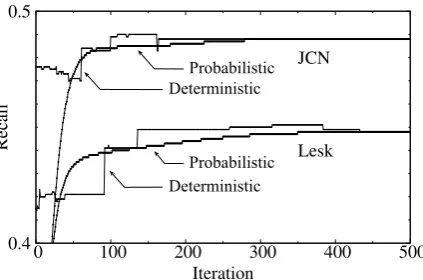
Figure 6: Recall improvement via iteration with SemEval-2 all POSs (JCN/k=30, Lesk/k=10).

with pseudo data in Section 3.2. Let us start by looking at the upper half of Figure 5, which shows the change of sense probabilities through itera-tion. At the initial status (iteration 0), the prob-abilities were all1/2for bi-semous words, all1/3

for tri-semous words, and so forth. As iteration proceeded, the probabilities gradually spread out to either side of 1 or 0, and finally at iteration 500, we can observe that almost all the words were clearly disambiguated. The lower half of Figure 5 shows the dynamics in bandwidths. Vertical axis on the left is for the sense bandwidth, and on the right is for the context bandwidth. We can ob-serve those bandwidths became narrower as iter-ation proceeded. Intensity of smoothing was dy-namically adjusted by the whole disambiguation status. These behaviors confirm that even with an actual dataset, it works as is expected, just as illus-trated in Figure 2.

6 Discussion

This section discusses the validity of the proposed method as to i) sense-interdependent disambigua-tion and ii) reliability of data smoothing. We here analyze the second peak conditions at k = 30

(JCN) andk= 10(Lesk) instead of the first peak

at k = 5, because we can observe tendency the

better with the larger number of word interactions.

6.1 Effects of Sense-interdependent Disambiguation

Let us first examine the effect of our sense-interdependent disambiguation. We would like to confirm that how the progressive disambigua-tion is carried out. Figure 6 shows the change of recall through iteration for JCN (k = 30) and

Lesk (k = 10). Those recalls were obtained by

evaluating the status after each iteration. The re-calls were here evaluated both in probabilistic for-mat and in deterministic forfor-mat. From the fig-ure we can observe that the deterministic recalls also increased as well as the probabilistic recalls. This means that the ranks of sense candidates for each word were frequently altered through itera-tion, which further means that some new infor-mation not obtained earlier was delivered one af-ter another to sense disambiguation for each word. From these results, we could confirm the expected sense-interdependency effect that a sense disam-biguation of certain word affected to other words.

6.2 Reliability of Smoothing as Supervision

Let us now discuss the reliability of our smoothing model. In our method, sense disambiguation of a word is guided by its nearby words’ extrapolation (smoothing). Sense accuracy fully depends on the reliability of the extrapolation. Generally speak-ing, statistical reliability increases as the number of random sampling increases. If we take suffi-cient number ofrandom words as nearby words, the sense distribution comes close to the true dis-tribution, and then we expect the statistically true sense distribution should find out the true sense of the target word, according to thedistributional hy-potheses (Harris, 1954). On the contrary, if we take nearby words that are biased to particular words, the sense distribution also becomes biased, and the extrapolation becomes less reliable.

We can compute the randomness of words that affect for sense disambiguation, by word per-plexity. Let the word of interest be w ∈ V. The word perplexity is calculated as2H|w, where H|w denotes the entropy defined as H|w ≡

−∑w′_∈V\{w}p(w′|w) log2p(w′|w). The

con-ditional probability p(w′|w) denotes the

proba-bility with which a certain word w′ _∈ V _\

{w_} determines the sense of w, which can be defined as the density ratio: p(w′|w) ∝

∑

i:wi=w

∑

i′:w_i′=w′

∑

j,j′Qi′j′(hij).

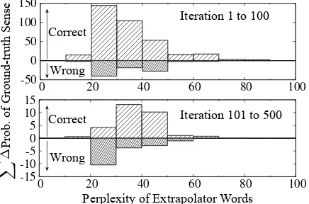
The relation between word perplexity and prob-ability change for ground-truth senses of nouns (JCN/k= 30) is shown in Figure 7. The upper

-15 -10 -5 0 5 10 15

0 20 40 60 80 100

-50 0 50 100 150

0 20 40 60 80 100

X

Iteration 1 to 100

Iteration 101 to 500

Perplexity of Extrapolator Words

P

rob. of G

round-t

rut

h S

ens

e

Correct

Wrong

Correct

Wrong

Figure 7: Correlation between reliability and per-plexity with SemEval-2 nouns (JCN/k= 30).

extend upward represent the sum of the amount raised (correct change), and the bars that extend downward represent the sum of the amount re-duced (wrong change). From these figures, we observe that when perplexity is sufficiently large (≥30), change occurred largely (79%) to the

cor-rect dicor-rection. In contrast, at the lower left of the figure, where perplexity is small (<30) and

band-widths has been narrowed at iteration 101-500, correct change occupied only 32% of the whole. Therefore, we can conclude that if sufficiently ran-dom samples of nearby words are provided, our smoothing model is reliable, though it is trained in an unsupervised fashion.

7 Related Work

As described in Section 1, graph-based WSD has been extensively studied, since graphs are favor-able structure to deal with interactions of data on vertices. Conventional studies typically consider as vertices the instances of input or target class, e.g. knowledge-based approaches typically regard senses as vertices (see Section 1), and corpus-based approaches such as (V´eronis, 2004) regard words as verticesor (Niu et al., 2005) regards con-text as vertices. Our method can be viewed as one of graph-based methods, but it regards input-to-class mapping as vertices, and the edges represent the relations both together in context and in sense. Mihalcea (2005) proposed graph-based methods, whose vertices are sense label hypotheses on word sequence. Our method generalize context repre-sentation.

In the evaluation, our method was compared to SemEval-2 systems. The main subject of the SemEval-2 task was domain adaptation, therefore

those systems each exploited their own adaptation techniques. Kulkarni et al. (2010) used a Word-Net pre-pruning. Disambiguation is performed by considering only those candidate synsets that be-long to the top-k largest connected components of the WordNet on domain corpus. Tran et al. (2010) used over 3TB domain documents acquired by Web search. They parsed those documents and extracted the statistics on dependency relation for disambiguation. Soroa et al. (2010) used the method by Agirre et al. (2009) described in Sec-tion 1. They disambiguated each target word us-ing its distributionally similar words instead of its immediate context words.

The proposed method is an extension of density estimation (Parzen, 1962), which is a construc-tion of an estimate based onobserved data. Our method naturally extends the density estimation in two points, which make it applicable to unsuper-vised knowledge-based WSD. First, we introduce stochastic treatment of data, which is no longer ob-servations but hypotheses having ambiguity. This extension makes the hypotheses possible to cross-validate the plausibility each other. Second, we extend the definition of density from Euclidean distance to general metric, which makes the pro-posed method applicable to a wide variety of corpus-based context similarities and dictionary-based sense similarities.

8 Conclusions

References

Eneko Agirre and Philip Edmonds. 2006. Word sense disambiguation: Algorithms and applications, vol-ume 33. Springer Science+ Business Media. Eneko Agirre and Aitor Soroa. 2009. Personalizing

pagerank for word sense disambiguation. In Pro-ceedings of the 12th Conference of the European Chapter of the Association for Computational Lin-guistics, pages 33–41.

Eneko Agirre, Oier Lopez De Lacalle, Aitor Soroa, and Informatika Fakultatea. 2009. Knowledge-based wsd on specific domains: performing better than generic supervised wsd. InProceedings of the 21st international jont conference on Artifical intel-ligence, pages 1501–1506.

Eneko Agirre, Oier Lopez de Lacalle, Christiane Fell-baum, Shu-Kai Hsieh, Maurizio Tesconi, Mon-ica Monachini, Piek Vossen, and Roxanne Segers. 2010. Semeval-2010 task 17: All-words word sense disambiguation on a specific domain. In Proceed-ings of the 5th International Workshop on Semantic Evaluation, pages 75–80.

Ted Briscoe, John Carroll, and Rebecca Watson. 2006. The second release of the rasp system. In Proceed-ings of the COLING/ACL on Interactive presenta-tion sessions, pages 77–80.

Arthur Pentland Dempster, Nan McKenzie Laird, and Donald Bruce Rubin. 1977. Maximum likelihood from incomplete data via the em algorithm. Journal of the Royal Statistical Society. Series B (Method-ological), pages 1–38.

Zellig Sabbetai Harris. 1954. Distributional structure. Word.

Jay J. Jiang and David W. Conrath. 1997. Semantic similarity based on corpus statistics and lexical tax-onomy. arXiv preprint cmp-lg/9709008.

Anup Kulkarni, Mitesh M. Khapra, Saurabh Sohoney, and Pushpak Bhattacharyya. 2010. CFILT: Re-source conscious approaches for all-words domain specific. In Proceedings of the 5th International Workshop on Semantic Evaluation, pages 421–426. Michael Lesk. 1986. Automatic sense disambiguation

using machine readable dictionaries: how to tell a pine cone from an ice cream cone. InProceedings of the 5th annual international conference on Systems documentation, pages 24–26.

Dekang Lin. 1998. Automatic retrieval and clustering of similar words. InProceedings of the 17th inter-national conference on Computational linguistics-Volume 2, pages 768–774.

Diana McCarthy, Rob Koeling, Julie Weeds, and John Carroll. 2004. Finding predominant word senses in untagged text. In Proceedings of the 42nd Annual Meeting on Association for Computational Linguis-tics, pages 279–286.

Diana McCarthy, Rob Koeling, Julie Weeds, and John Carroll. 2007. Unsupervised acquisition of pre-dominant word senses. Computational Linguistics, 33(4):553–590.

Rada Mihalcea. 2005. Unsupervised large-vocabulary word sense disambiguation with graph-based algo-rithms for sequence data labeling. InProceedings of the conference on Human Language Technology and Empirical Methods in Natural Language Pro-cessing, pages 411–418.

Roberto Navigli and Mirella Lapata. 2007. Graph connectivity measures for unsupervised word sense disambiguation. In Proceedings of the 20th inter-national joint conference on Artifical intelligence, pages 1683–1688.

Roberto Navigli. 2009. Word sense disambiguation: A survey. ACM Computing Surveys (CSUR), 41(2):10.

Zheng-Yu Niu, Dong-Hong Ji, and Chew Lim Tan. 2005. Word sense disambiguation using label prop-agation based semi-supervised learning. In Pro-ceedings of the 43rd Annual Meeting on Association for Computational Linguistics, pages 395–402.

Emanuel Parzen. 1962. On estimation of a probability density function and mode. The annals of mathe-matical statistics, 33(3):1065–1076.

Siddharth Patwardhan, Satanjeev Banerjee, and Ted Pedersen. 2007. UMND1: Unsupervised word sense disambiguation using contextual semantic re-latedness. Inproceedings of the 4th International Workshop on Semantic Evaluations, pages 390–393.

Ted Pedersen, Siddharth Patwardhan, and Jason Miche-lizzi. 2004. WordNet::Similarity: measuring the re-latedness of concepts. In Demonstration Papers at HLT-NAACL 2004, pages 38–41.

Aitor Soroa, Eneko Agirre, Oier Lopez de Lacalle, Monica Monachini, Jessie Lo, Shu-Kai Hsieh, Wauter Bosma, and Piek Vossen. 2010. Kyoto: An integrated system for specific domain WSD. In Pro-ceedings of the 5th International Workshop on Se-mantic Evaluation, pages 417–420.

Andrew Tran, Chris Bowes, David Brown, Ping Chen, Max Choly, and Wei Ding. 2010. TreeMatch: A fully unsupervised WSD system using dependency knowledge on a specific domain. InProceedings of the 5th International Workshop on Semantic Evalu-ation, pages 396–401.