Rich Prior Knowledge in
Learning for NLP
Gregory Druck, Kuzman Ganchev, João Graça
Why Incorporate Prior Knowledge?
have: unlabeled data
option: hire
Why Incorporate Prior Knowledge?
have: unlabeled data
option: hire
linguist annotators
This approach does not scale to every task and domain of interest.
However, we already know a lot about most problems of interest.
Example: Document Classification
•
Prior Knowledge:•
labeled features: information about the label distribution when word w is present--- --- --- -- -- --- ---- --- --- --- --- -- --- --- ---- --
--- --- --- -- -- --- ---- --- --- --- --- -- --- --- ---- --
--- --- --- -- -- --- ---- --- --- --- --- -- --- --- ---- --
--- --- --- -- -- --- ---- --- --- --- --- -- --- --- ---- --
--- --- --- -- -- --- ---- --- --- --- --- -- --- --- ---- --
--- --- --- -- -- --- ---- --- --- --- --- -- --- --- ---- --
Documents Labels
newsgroups classification
baseball Mac politics ...
hit Apple senate ...
Braves Macintosh taxes ...
runs Powerbook liberal ... sentiment polarity
positive negative
memorable terrible
perfect boring
Example: Information Extraction
•
Prior Knowledge:•
labeled features:•
the word ACM should be labeled either journal orbooktitle most of the time
•
non-Markov (long-range) dependencies:•
each reference has at most one segment of each typeW. H. Enright.Improving the efficiency of matrix operations in the numerical solution of stiff ordinary differential equations.ACM Trans. Math. Softw.,4(2),127-136,June 1978. extraction from
research papers:
Example: Part-of-speech Induction
•
Prior Knowledge:•
linguistic knowledge: each sentence should have a verb•
posterior sparsity: the total number of different POS tagsassigned to each word type should be small
Tags
A career with the European institutions must become more
Example: Dependency Grammar Induction
•
Prior Knowledge:•
linguistic rules: nouns are usually dependents of verbs•
noisy labeled data: target language parses should besimilar to aligned parses in a resource-rich source language
Example: Word Alignment
•
Prior Knowledge:•
Bijectivity: alignment should be mostly one-to-one•
Symmetry: source→target and target→sourcealignments should agree
Acareerwith theEuropeaninstitutionsmust becomemoreattractive.
This Tutorial
In general, how can we leverage such knowledge
and an unannotated corpus during learning?
Notation & Models
input variables (documents, sentences):
structured output variables (parses, sequences): unstructured output variables (labels):
input / output variables for entire corpus: probabilistic model parameters:
generative models: discriminative models: model feature function:
p
θ(
y
|
x
)
p
θ(
x
,
y
)
x
y
θ
f
(
x
,
y
)
X Y
Learning Scenarios
•
Unsupervised:•
unlabeled data + prior knowledge•
Lightly Supervised:•
unlabeled data + “informative” prior knowledge•
i.e. provides specific information about labels•
Semi-Supervised:•
labeled data + unlabeled data + prior knowledgeRunning Example #1:
Document Classification
•
model: Maximum Entropy Classifier (Logistic Regression)•
setting: lightly supervised; no labeled data•
prior knowledge:•
labeled features: information about the label distribution when word w is present•
label is often hockey or baseball when game is presentpθ(y|x) =
1
Running Example #2:
Word Alignment
•
model: first-order Hidden Markov Model (HMM)•
setting: unsupervised•
prior knowledge:•
Bijectivity: alignment should be mostly one-to-one1 1 2 3
we know the way sabemos el camino null
1 2 3 0
pθ(y,x) = pθ(y0) N
�
i=1
pθ(yi|yi−1)pθ(xi|yi)
Problem
This output does not agree with prior knowledge!
•
six target words align to source word animada•
five source words do not align with any target word game convivialvery
,
animated an was it
cordial
muy
y
animada
manera una de jugaban
model
data
output
x1 x2 x3
y1 y2 y3
Limited Approach: Labeling Data
limitation: Often unclear how to do conversion
•
Example #1: often (not always) game → {hockey,baseball}•
Example #2: alignment should be mostly one-to-oneprior knowledge --- --- --- -- -- --- ---- --- --- --- --- -- --- --- ---- -- --- --- --- -- -- --- ---- --- --- --- --- -- --- --- ---- -- --- --- --- -- -- --- ---- --- --- --- --- -- --- --- ---- -- --- --- --- -- -- --- ---- --- --- --- --- -- --- --- ---- -- --- --- --- -- -- --- ---- --- --- --- --- -- --- --- ---- -- --- --- --- -- -- --- ---- --- --- --- --- -- --- --- ---- --
approach: Convert prior knowledge to labeled data.
Prototypes (+ cluster features):
•
[Haghighi & Klein 06]Others:
•
[Raghavan & Allan 07]•
[Schapire et al. 02]Limited Approach: Bayesian Approach
approach: Encode prior knowledge with a prior on parameters.
limitation: Our prior knowledge is not about parameters! Parameters are difficult to interpret; hard to get desired effect.
•
Example #1: often (not always) game → {hockey,baseball}•
Example #2: alignment should be mostly one-to-onenatural: “ should be θ small (or sparse)”
( informative prior )
possible: “ should be close to ”θi θ˜i
p(θ)
specifying
x1 x2 x3 y1 y2 y3
θ α
Limited Approach: Augmenting Model
limitation: can be difficult to get desired effect
•
Example #1: often (not always) game → {hockey,baseball}limitation: may make exact inference intractable
•
Example #2: Bijectivity makes inference #P-completex1 x2 x3
y1
y2 y3 z1
approach: Encode prior knowledge with additional variables and dependencies.
This Tutorial
develop:
•
a language for directly encoding prior knowledge•
methods for learning with knowledge in this language•
( approximations to modeling this language directly )•
(loosely) these methods perform mappings for us:•
encoded prior knowledge parameters•
encoded prior knowledge labelingθ
--- --- --- -- --
--- ---- --- --- --- --- --- --- -- --
--- ---- --- --- ---
--- --- --- -- --
--- ---- --- --- ---
A Language for Encoding Prior Knowledge
Our prior knowledge is about distributions over latent output variables. (output variables are interpretable)
Specifically, we know some properties of this distribution:
•
Example #1: often (not always) game→{hockey,baseball}Formulation: know about the expectations of some functions under distribution over latent output variables
Constraint Features
•
constraint feature function:•
Example #1:•
for document x, returns a vector with a 1 in the lthposition if y is the lth label and the word w is in x
•
Example #2:•
returns a vector with mth value = number of target words in sentence x that align with source word mφ
(
x
,
y
)
φw(x, y) = 1(y = l)1(w ∈ x)
φ(x,y) =
N
�
i=1
Expectations of Constraint Features
•
Example #1: Corpus expectation:•
vector with expected distribution over labels for documents that contain w ( is the count of w)•
Example #2: Per-example expectation:•
vector with mth value = expected number of target words that align with source word mEpθ[φ(X,Y)] =
1
cw
�
x
�
y
pθ(y|x)φw(x, y)
Epθ[φ(x,y)] =
�
y
pθ(y|x)φ(x,y)
cw
Expressing Preferences
•
express preferences using target values:•
Example #1:•
label distribution for game is close to [40% 40% 20%]•
Example #2:•
expected number of target words that align with each source word is at most one˜
φ
Epθ[φw(X,Y)] ≈ φ˜
Preview: Labeled Features
User Experiments [Druck et al. 08]
0 100 200 300 400 500 600 700 800 0.4
0.5 0.6 0.7 0.8 0.9 1
labeling time in seconds
testing accuracy
GE ER ~2 minutes, 100
features labeled (or skipped): 82% accuracy
~15 minutes, 100 documents labeled
(or skipped): 78% accuracy
PC vs. Mac
complete set of labeled features
PC Mac
dos mac
ibm apple
hp quadra
dx
targetsset with simple heuristic: majority label gets
90% of mass
Preview: Word Alignment
[Graça et al. 10]
60 68.75 77.5 86.25 95
En-Pt Pt-En En-Es Es-En
Overview of the Frameworks
Running Example
Model Family:
conditional exponential models
are
model
features
p
θ(
Y
|
X
) =
exp(θ
·
f
(
X
,
Y
))
Z
(
X
)
Z
(
X
) =
�
Y
exp(θ
·
f
(
X
,
Y
))
Choosing parameters
Model Family
:
conditional exponential models
Objective
:
maximize observed data likelihood
Note:
Frameworks also suitable for
generative models (no labeled data necessary)
θ
p
θ(
Y
|
X
) =
exp(θ
·
f
(
X
,
Y
))
Z
(
X
)
max
θ
log
p
θ(
Y
L|
X
L) + log
p
(
θ
)
def
=
L
(θ;
D
L)
Visual Example: Maximum Likelihood
Model:
Objective:
-+
o
o
o
o
o
o
o
o
max
θ
log
p
θ(
Y
L|
X
L)
−
0.1
�
θ
�
2 2
p
(
Y
|
X
) =
�
i
exp(
y
ix
i·
θ
)
A language for prior information
The expectations of user-defined
constraint
features are close to some value
φ
(
X
,
Y
)
φ
˜
E
[
φ
(
X
,
Y
)]
≈
φ
˜
Running Example:
Want to ensure that 25% of unlabeled
documents are about politics
•
constraint
features
•
preferred expected value
•
Expectation w.r.t. unlabeled data
φ
(
x
,
y
) =
�
1 if
y
is “politics”
0 otherwise
˜
Constraint-Driven Learning
Motivation
:
Hard EM algorithm with preferences
Hard EM
:
Constraint Driven Learning
:
M-Step: set
θ
= arg max
θ
log
p
θ( ˆ
Y
|
X
)
E-Step: set ˆ
Y
= arg max
Y
log
p
θ(
Y
|
X
)
−
penalty(
Y
)
M-Step: set
θ
= arg max
θ
log
p
θ( ˆ
Y
|
X
)
E-Step: set ˆ
Y
= arg max
Y
log
p
θ(
Y
|
X
)
M. Chang, L. Ratinov, D. Roth (2007).
Constraint-Driven Learning
Motivation
:
Hard EM algorithm with preferences
Constraint Driven Learning
:
•
penalties encode similar information as
•
E-Step can be hard; use beam search
E-Step: set ˆ
Y
= arg max
Y
log
p
θ(
Y
|
X
)
−
penalty(
Y
)
M-Step: set
θ
= arg max
θ
log
p
θ( ˆ
Y
|
X
)
Visual Example: Constraint Driven Learning
where are “imagined” labels and
Y
ˆ
-+
o
o
o
o
o
o
o
o
φ[ ˆ
Y
] = count(+,
Y
ˆ
)
max
θ,Yˆ
log
p
θ(
Y
L|
X
L)
−
0
.
1
�
θ
�
22s.t.
φ
( ˆ
Y
) = 2
Posterior Regularization
Motivation
:
EM algorithm with
sane
posteriors
EM:
Constrained EM:
E-Step: set
q
(
Y
) = arg min
q
D
KL(
q
(
Y
)
||
p
θ(
Y
|
X
))
M-Step: set
θ
= arg max
θ
E
q(Y)[
p
θ(
Y
|
X
)]
E-Step: set
q
(
Y
) = arg min
q∈Q
D
KL(
q
(
Y
)
||
p
θ(
y
|
x
))
M-Step: set
θ
= arg max
θ
Posterior Regularization
Motivation
:
EM algorithm with
sane
posteriors
Idea:
provide constraints
Objective:
E
[
φ
]
≈
φ
˜
define
Q
: set of
q
such that
E
q[
φ
]
≈
φ
˜
max
θ
L
(
θ
;
D
L)
−
D
KL(
Q ||
p
θ(
Y
|
X
))
run EM-like procedure but use proposal
q
∈
Q
where
D
KLis Kullback-Leibler divergence
X
=
D
Uare the input variables for unlabeled corpus
Y
is label for
entire
unlabeled corpus
Posterior Regularization
Hard constraints:
Soft constraints:
max
θ
L
(θ;
D
L)
−
min
q∈QD
KL(
q
(
Y
)
||
p
θ(
Y
|
X
))
Q
=
�
q
(
Y
) :
�
�
�
E
q[
φ
(
Y
)] = ˜
φ
�
�
�
22
≤
�
�
max
θ
L
(
θ
;
D
L)
−
min
q�
D
KL(
q
(
Y
)
||
p
θ(
Y
|
X
)) +
α
�
�
�
E
q[
φ
(
Y
)] = ˜
φ
�
�
�
22
Visual Example: Posterior Regularization
where:
-+
o
o
o
o
o
o
o
o
max
θ
log
p
θ(
Y
L|
X
L)
−
0
.
1
�
θ
�
2
2
−
D
KL(
Q||
p
θ)
D
KL(
Q||
p
θ) = min
q
D
KL(
q
||
p
θ) s.t.
E
q[φ] = 2
Generalized Expectation Constraints
Motivation
:
augment log-likelihood with cost for “bad”
posteriors.
Objective:
where
is short-hand
Optimization:
gradient descent on
max
θ
L
(
θ
;
D
L)
−
�
�
�
E
pθ(Y|X)[
φ
]
−
φ
˜
�
�
�
β
E
pθ(Y|X)[
φ
] =
E
pθ(Y|X)[
φ
(
X
,
Y
)]
=
�
Y
p
θ(
Y
|
X
)
φ
(
X
,
Y
)
θ
A visual comparison of the frameworks
Objective:
Generalized Expectation Constraints
-+
o
o
o
o
o
o
o
o
max
θ
log
p
θ(
Y
L|
X
L)
−
0
.
1
�
θ
�
22
−
500
�
E
pθ[
φ
]
−
2
�
2 2
Types of constraints
Constraint Driven Learning:
Penalized Viterbi
•
Easy if decompose as the model.
and
•
Otherwise:
•
Beam search
•
Integer linear program
p
(
Y
|
X
) =
�
c
p
c(
y
c|
X
)
arg max
Y
log
p
θ(
Y
|
X
)
− �
φ
(
X
,
Y
)
−
φ
˜
�
β�
φ
(
X
,
Y
)
−
φ
˜
�
β�
φ
(
X
,
Y
)
−
φ
˜
�
β=
�
c
Types of constraints
Posterior Regularization:
KL projection
•
Usually easy if decompose as the model:
and
•
Otherwise: Sample
(e.g. K. Bellare, G. Druck, and A. McCallum, 2009)φ
(
Y
,
X
)
p(Y|X) = �
c
pc(yc|X)
q(Y|X) = �
c
qc(yc|X)
φ(X,Y) = �
c
φc(X,yc)
⇒
min
q
D
KL(
q
||
p
θ) s.t.
�
E
q[
φ
]
−
˜
φ
�
β≤
�
Types of constraints
Generalized Expectation Constraints:
Direct gradient
•
Usually easy if:
•
decomposes as the model
•
Can compute
•
Unstructured
•
Sequence, Grammar (semiring trick)
•
Otherwise: sample or approximate the gradient.
φ
(
Y
,
X
)
max
θ
L
(
θ
;
D
L)
−
�
�
�
E
pθ(Y|X)[
φ
]
−
φ
˜
�
�
�
β
φ(X,Y) = �
c
φc(X,yc)
A Bayesian View: Measurements
Objective:
mode of given observations
XL θ X
YL Y
φ(X,Y)
[image:22.612.74.540.54.772.2]b
Figure 4.1: The model used by Liang et al. [2009], using our notation. We have separated treatment of the labeled data (XL,YL)from treatment of the unlabeled data X.
and produce some value φ(X,Y), which is never observed directly. Instead, we observe some noisy version b ≈ φ(X,Y). The measured values b are distributed according to
some noise modelpN(b|φ(X,Y)). Liang et al. [2009] note that the optimization is convex
for log-concave noise and use box noise in their experiments, givingbuniform probability
in some range near φ(X,Y).
In the Bayesian setting, the model parameters θ as well as the observed measurement valuesbare random variables. Liang et al. [2009] use the mode of p(θ|XL,YL,X,b) as a
point estimate forθ:
arg max θ
p(θ|XL,YL,X,b) = arg max
θ
�
Y
p(θ,Y,b|X,XL,YL), (4.6)
with equality because p(θ|XL,YL,X,b) ∝ p(θ,b|XL,YL,X) =
�
Yp(θ,Y,b|X,XL,YL). Liang et al. [2009] focus on computingp(θ,Y,b|X,XL,YL). They define their model for this quantity as follows:
p(θ,Y,b|X,XL,YL) = p(θ|XL,YL) pθ(Y|X) pN(b|φ(X,Y)) (4.7)
where theY andXare particular instantiations of the random variables in the entire
unla-beled corpusX. Equation 4.7 is a product of three terms: a prior onθ, the model probability
pθ(Y|X), and a noise model pN(b|φ). The noise model is the probability that we observe
a value, b, of the measurement features φ, given that its actual value was φ(X,Y). The idea is that we model errors in the estimation of the posterior probabilities as noise in the measurement process. Liang et al. [2009] use a uniform distribution over φ(X,Y) ± �, which they call “box noise”. Under this model, observing b farther than � from φ(X,Y) has zero probability. In log space, the exact MAP objective, becomes:
max
θ L(θ) + logEpθ(Y|X)
�
pN(b|φ(X,Y))
�
. (4.8)
31
max
θ logp(θ) +
�
(x,y)∈DL
logpθ(y|x) = L(θ;DL)
θ
P. Liang, M. Jordan, D. Klein (2009)
Objective:
mode of given observations
A Bayesian View: Measurements
XL θ X
YL Y
φ(X,Y)
b
Figure 4.1: The model used by Liang et al. [2009], using our notation. We have separated treatment of the labeled data(XL,YL) from treatment of the unlabeled dataX.
and produce some value φ(X,Y), which is never observed directly. Instead, we observe some noisy version b ≈ φ(X,Y). The measured values b are distributed according to
some noise modelpN(b|φ(X,Y)). Liang et al. [2009] note that the optimization is convex
for log-concave noise and use box noise in their experiments, giving buniform probability
in some range near φ(X,Y).
In the Bayesian setting, the model parameters θ as well as the observed measurement
values bare random variables. Liang et al. [2009] use the mode ofp(θ|XL,YL,X,b)as a
point estimate forθ:
arg max θ
p(θ|XL,YL,X,b) = arg max
θ
�
Y
p(θ,Y,b|X,XL,YL), (4.6)
with equality because p(θ|XL,YL,X,b) ∝ p(θ,b|XL,YL,X) =
�
Y p(θ,Y,b|X,XL,YL). Liang et al. [2009] focus on computingp(θ,Y,b|X,XL,YL). They define their model for this quantity as follows:
p(θ,Y,b|X,XL,YL) = p(θ|XL,YL) pθ(Y|X) pN(b|φ(X,Y)) (4.7)
where the Y and X are particular instantiations of the random variables in the entire
unla-beled corpusX. Equation 4.7 is a product of three terms: a prior onθ, the model probability
pθ(Y|X), and a noise model pN(b|φ). The noise model is the probability that we observe
a value, b, of the measurement features φ, given that its actual value was φ(X,Y). The idea is that we model errors in the estimation of the posterior probabilities as noise in the measurement process. Liang et al. [2009] use a uniform distribution over φ(X,Y) ± �,
which they call “box noise”. Under this model, observing b farther than � from φ(X,Y) has zero probability. In log space, the exact MAP objective, becomes:
max
θ L(θ) + logEpθ(Y|X) �
pN(b|φ(X,Y))
�
. (4.8)
31 max
θ L(θ;DL) + logEpθ(Y|X) �
What's wrong with this picture?
Objective:
mode of given observations
Example:
Exactly 25% of articles are “politics”
What is the probability exactly 25% of the articles are
labeled ``politics''?
How do we optimize this with respect to ?
max
θ
L
(
θ
;
D
L) + logE
pθ(Y|X)�
p
( ˜
φ
|
φ
(
X,
Y
))
�
θ
θ
p( ˜
φ
|
φ
(
X
,
Y
)) =
1
�
φ
˜
=
φ
(
X
,
Y
)
�
E
pθ(Y|X)�
1
( ˜
φ
=
φ
(
X
,
Y
))
�
What's wrong with this picture?
Example:
Compute prob: 25% of docs are “politics”.
Naively:
in this case we can use a DP, but if
there are many constraints, that doesn’t
work.
Easier:
What is the expected number of “politics” articles?
Article p(“politics”)
1
0.2
2
0.4
3
0.1
4
0.6
0.2 + 0.4 + 0.1 + 0.6
Probabilities and Expectations
difficult to compute expectations of arbitrary functions
but
...
Usually:
decomposes as a sum
e.g.
25% of articles are “politics”
Idea:
approximate
φ(X,Y)
φ(X,Y) = �
instances
φ(x,y)
Epθ(Y|X)�p�φ˜
|
φ(X,Y)��≈ p�φ˜|
Epθ(Y|X)[φ(X,Y)]�Probabilities and Expectations
Approximation:
Objective:
Example:
is Gaussian
is
so for appropriate this is identical to GE!
Epθ(Y|X)
�
p�φ˜
|
φ�� ≈ p�φ˜|
Epθ(Y|X)[φ]�
max
θ
L
(
θ
;
D
L) + log
p
�
˜
φ
|
E
pθ(Y|X)[
φ
]
�
log
p
�
φ
˜
|
E
[φ]
�
⇒
p�φ˜
|
E[φ]�logp�φ˜
|
E[φ]�⇓
� �
�E[φ]−φ˜���2
Optimizing GE objective
GE Objective:
•
Gradient involves covariance
this can be hard because
and the usual dynamic programs (inside outside, forward
backward) can’t compute this.
Cov(
φ
,
f
) =
E
[
φ
×
f
]
−
E
[
φ
]
×
E
[
f
]
E
[
φ
×
f
] =
�
Y
p
(
Y
)
φ
(
Y
)
×
f
(
Y
)
O
GE= max
θ
L
(
θ
;
D
L)
−
�
�
�
E
pθ(Y|X)[
φ
(
X
,
Y
)]
−
φ
˜
�
�
�
β
Optimizing GE Objective
Maintaining both and in the DP is expensive
*
Semiring trick can help for some problems
*
x1 x2 x3 x3y1 y2 y3 y4
E[φ×f] =�
Y
p(Y)φ(Y)×f(Y)
φ(Y)×f(Y) =
� �
i
φ(yi)
�
×
�
j
f(yj)
y
iy
jA Variational Approximation
GE Objective:
•
Can be hard to compute in gradient.
Idea:
use variational approximation
*
Note: this is the PR objective
*
q
(
Y
)
≈
p
θ(
Y
|
X
)
maxθ,q(Y) L(θ;DL)−DKL�q(Y)
||
pθ(Y|X)�−� �
�Eq[φ(X,Y)] − φ˜
� � �
β
Cov(
φ,
f
)
O
GE= max
θ
L
(
θ
;
D
L)
−
�
�
�
φ
˜
−
E
pθ(Y|X)[
φ
(
X
,
Y
)]
�
�
�
β
Approximating with the mode
PR Objective:
sometimes minimizing the KL is hard.
Idea:
use hard assignment :
•
becomes
•
becomes
•
use EM-like procedure to optimize
Constraint Driven Learning Objective:
maxθ,q(Y) L(θ;DL)−DKL�q(Y)||
pθ(Y|X)�−� �
�Eq[φ(X,Y)] − φ˜
� � �
β
q
(
Y
)
≈
1
(
Y
= ˆ
Y
)
�
�
�
E
q[
φ
(
X
,
Y
)]
−
φ
˜
�
�
�
β
log
p
( ˆ
Y
)
D
KL�
q
(
Y
)
||
p
θ(
Y
|
X
)
�
log
p
( ˜
φ
|
φ
(
X
,
Y
ˆ
))
max
θ,Yˆ
L
Visual Summary
Measurements
Generalized
Expectation
Distribution Matching
Posterior
Regularization
Coupled Semi-Supervised
Learning
Constraint
Driven
Learning Distribution
Matching
variational approximation; Jensen’s inequality
variational approximation
MAP approximation
MAP approximation logE[pN( ˜φ|φ)]≈ logpN( ˜φ|E[φ])
Applications
•
Unstructured problems:•
Document Classification•
Sequence problems:•
Information Extraction•
Pos-Induction•
Word Alignment•
Tree problems:Document Classification
•
Model: Max. Entropy Classifier (Logistic Regression)•
Challenge:What if we have no labeled data?•
cannot use standard unsupervised learning:--- --- --- -- -- --- ---- --- --- --- --- -- --- --- ---- --
--- --- --- -- -- --- ---- --- --- --- --- -- --- --- ---- --
--- --- --- -- -- --- ---- --- --- --- --- -- --- --- ---- --
--- --- --- -- -- --- ---- --- --- --- --- -- --- --- ---- --
--- --- --- -- -- --- ---- --- --- --- --- -- --- --- ---- --
--- --- --- -- -- --- ---- --- --- --- --- -- --- --- ---- --
Documents Labels
pθ(y|x) =
exp(θ ·f(x, y))
�
yexp(θ ·f(x, y))
�
y
pθ(y|x) = 1
Labeled Features
•
often we can still provide some light supervision•
prior knowledge: labeled features•
formally: have an estimate of the distribution over labels for documents that contain word w: φ˜wnewsgroups classification
baseball Mac politics ...
hit Apple senate ...
Braves Macintosh taxes ...
runs Powerbook liberal ... sentiment polarity
positive negative
memorable terrible
perfect boring
Leveraging Labeled Features with GE
[Mann & McCallum 07], [Druck et al. 08]
•
constraint feature:•
for a document x, returns a vector with a 1 in the lthposition if y is the lth label and the word w is in x
•
expectation: label distribution for docs that contain w•
GE penalty: KL divergence from target distributionφw(x, y) = 1(y = l)1(w ∈ x)
1
cw
�
x
Epθ(y|x)[φw(x, y)]
DKL
�˜
φw||
1 cw
�
x
Epθ(y|x)[φw(x, y)]
�
User Experiments with Labeled Features
[Druck et al. 08]
0 100 200 300 400 500 600 700 800 0.4
0.5 0.6 0.7 0.8 0.9 1
labeling time in seconds
testing accuracy
GE ER ~2 minutes, 100
features labeled (or skipped): 82% accuracy
~15 minutes, 100 documents labeled
(or skipped): 78% accuracy
PC vs. Mac
complete set of labeled features
PC Mac
dos mac
ibm apple
hp quadra
dx
targetsset with simple heuristic: majority label gets
Experiments with Labeled Features
[Druck et al. 08]
60 65 70 75 80
sentiment (50) webkb (100) newsgroups (500) GE (model contains only labeled features) GE (model also contains unlabeled features)
15x
3.5x
6.5x
learning about “unlabeled features” through covariance improves generalization estimated speed-up over
labeling documents
Information Extraction: Example Tasks
•
citation extraction:•
apartment listing extraction:Detached single family house. 3 bedrooms 1 1/2 baths. Almost 1000 square feet in living area.1 car garage. New pergo floor and tile kitchen floor. New interior/exterior paint.Close to shopping mall and bus stop. Near 101/280.Available July 1, 2004.If you are interested, email for more details.
Cousot, P. and Cousot, R. 1978.Static determination of
Information Extraction: Markov Models
•
models for sequence labeling based IE•
Hidden Markov Model (HMM):•
Conditional Random Field (CRF):pθ(y,x) = pθ(y0) N
�
i=1
pθ(yi|yi−1)pθ(xi|yi)
pθ(y|x) = 1
Z(x) exp( N
�
i=1
θ·f(x, yi−1, yi))
expectation:
label distribution when q is true
model: Linear Chain CRF
note: Semiring trick makes GE O(L2) instead of O(L3) as in
[Mann & McCallum 08]
Information Extraction: Labeled Features
[Mann & McCallum 08], [Liang et al. 09]
ROOMMATES respectful
CONTACT *phone*
FEATURES laundry
apartments example labeled features:
1
cq
�
x
�
i
Epθ(yi|x)[φq(x, yi, i)]
constraint features:
vector with a 1 in the lth
position if y is the lth label and predicate q is true (i.e. w
is present at i)
Information Extraction: Labeled Features
[Haghighi & Klein 06], [Mann & McCallum 08], [Liang et al. 09]
apartment listing extraction
Prototype GE (KL)
Measurements/PR
650 700 750 800 850
0 labeled 10 labeled 100 labeled
supervised CRF (100) [MM08]
•
accurate with constraints alone•
outperform fully supervised withconstraints and labeled data
Limitations of Markov Models
•
predicted:•
prediction has two author and two title segments:•
error #1: Neuhold, Ed. should be editor•
error #2: North-Holland Pub. Co., should bepublisher
•
A Markov model cannot represent that at most one segmentof each type appears in each reference.
Long-Range Constraints
[Chang et al. 07] [Bellare et al. 09]
•
“Each field is a contiguous sequence of tokens and appears at most once in a citation.”•
constraint feature: counts the number of segments of each type•
constrained to be ≤ 1 using PR or CODL•
additional constraints: 10 labeled features such as:•
pages→pages•
proc.→booktitleLong-Range Constraints
[Chang et al. 07] [Bellare et al. 09]
constraints improve both CRF (PR) and HMM (CODL)
50 60 70 80 90
5 labeled 20 labeled
CRF CRF + PR
citation model method description
[Mann et al. 07] MaxEnt GE label marginalsconstraints on
[Druck et al. 09] CRF GE actively labeled features
[Bellare &
McCallum 09] alignment CRF GE labeled features
[Singh et al. 10] semi-Markov CRF PR labeled gazetteers
[Druck et al. 10] HMM PR constraints derived from labeled data
Other Applications in
Information Extraction
Pos Induction
Low Tag Ambiguity
[Graça et al. 09]
JJ
VB
NN
car object
romantic offensive
being E[degree] = 1.5 E[degree] = 10000
0 2 4 6 8 10
0 200 400 600 800 1000 1200 1400 1600 1800 L1
L!
rank of word by L1L! Supervised
HMM
N V ADJ Prep ADV 0.9 0.1 0 0 0 0.7 0.1 0.1 0 0.1 0.1 0.3 0 0.6 0 0.3 0.6 0 0 0.1 0.3 0.7 0 0 0
•
Pick a particular word type: run•
Stack all occurrences•
Calculate posterior probability•
Take the maximum for each tag•
Sum the maxesa run into town. of the mile run.
run gold.
run errands.
run for mayor.
Sum 1 Sum 1 1 1 1 1
0.9 0.7 0.1 0.6 0.2
Max
Sum
2.5
Measuring Tag Ambiguity
[Graça et al. 09]
φ
wti :Word type w has hidden state t at occurrence imin
cwt
E
q(y)[
φ
wti]
≤
c
wt�
1/
�
∞=
�
wt
c
wtTag Sparsity
[Graça et al. 09]
0 1.25 2.5 3.75 5
En Pt Es
Ambi gui ty di ffer ence HMM L1LMax Average ambiguity difference 0 2 4 6 8 10
0 200 400 600 800 1000 1200 1400 1600 1800 L1
L!
rank of word by L1L! Supervised
HMM HMM+Sp
Results
[Graça et al. 09]
50 57.5 65 72.5 80
En Pt Bg Es Dk Tr
HMM HMM+Sp
3.8 6.7
7.4
7.6 9.6
3.8
6.5 % Average Improvement
Word Alignments
[Graça et al. 10]
•
Bijectivity constraints:
•
Each word should align to at most one other word•
Symmetry constraints:Bijectivity Constraints
[Graça et al. 10] Bijective Constraints
0 1 2 3 4 5 6 7 8
0 � � ♣ ♣ ♣ ♣ ♣ ♣ ♣ jugaban �≤1 1 ♣ ♣ ♣ ♣ ♣ ♣ ♣ ♣ ♣ de �≤1 2 ♣ ♣ � ♣ ♣ ♣ ♣ ♣ ♣ una �≤1 3 � ♣ � ♣ ♣ ♣ ♣ ♣ ♣ manera �≤1 4 � ① ✇ ① ♣ ♣ ① ① ♣ animada �≤1 5 ♣ ♣ ♣ ♣ ① ♣ ♣ ♣ ♣ y �≤1 6 ♣ ♣ ♣ ♣ ♣ ① ♣ ♣ ♣ muy �≤1 7 ♣ ♣ ♣ ♣ ♣ � ♣ � ♣ cordial �≤1 8 ♣ ♣ ♣ ♣ ♣ ♣ ♣ ♣ ①. �≤1
it wa san animat
ed , very con
vivgaialme .
50 / 74
Bijective Constraints - After projection
0 1 2 3 4 5 6 7 8
0 � ♣ ♣ ♣ ♣ ♣ � � ♣ jugaban �≤1 1 � � ♣ ♣ ♣ ♣ ♣ ♣ �de �≤1 2 ♣ ♣ ① ♣ ♣ ♣ ♣ ♣ ♣ una �≤1 3 ♣ � ♣ ♣ ♣ ♣ ♣ ♣ ♣ manera �≤1 4 ♣ ♣ ♣ ③ ♣ ♣ ♣ ♣ ♣ animada �≤1 5 ♣ ♣ ♣ ♣ ① ♣ ♣ ♣ ♣ y �≤1 6 ♣ ♣ ♣ ♣ ♣ ③ ♣ ♣ ♣ muy �≤1 7 ♣ ♣ ♣ ♣ ♣ ♣ ① ✈ ♣ cordial �≤1 8 ♣ ♣ ♣ ♣ ♣ ♣ ♣ ♣ ✇. �≤1
it wa san animat
ed , very con
viv ial ga
me.
51 / 74
Feature: Constraint:
φ(x,y) =
N
�
i=1
1(yi = m)
Eq[φ(x,y)] ≤ 1
Symmetry Constraints
[Graça et al. 10]
Feature:
Constraint:
Symmetric - Original posteriors
0 1 2 3 4
− →pθt(z|x)
0 ① ♣ ♣ ♣ ♣ no
1 � ♣ � � ♣ hay
2 ♣ ① ① ① ♣ estad´ısticas
3 ♣ ♣ ♣ ♣ ①.
0 1 2 3 4
←−pθt(z|x)
0 ① ♣ ♣ ♣ ♣ no
1 � � ♣ � ♣ hay
2 ♣ ✇ � � ♣ estad´ısticas
3 ♣ ♣ ♣ ♣ ①. no sta
tistica l data exi
sts.
pθt q
←− pθt
−→
pθt
55 / 74
E
q[
φ
(
x
,
y
)] = 0
φ(x,y) =
+1 y ∈ −→y and −→y i = j
−1 y ∈ ←−y and ←−y j = i 0 otherwise
−
→pθ(y|x)
Symmetry Constraints
[Graça et al. 10]
Before projection: After projection:
Symmetric - After projection
E-Step qs(z) = arg min q(z)∈Qs
KL[qs(z)||pθt(z|xs)]
0 1 2 3 4
− →pθt(z|x)
0 ① ♣ ♣ ♣ ♣ no
1 � ♣ � � ♣ hay
2 ♣ ① ① ① ♣ estad´ısticas
3 ♣ ♣ ♣ ♣ ①.
0 1 2 3 4
←−pθt(z|x)
0 ① ♣ ♣ ♣ ♣ no
1 � � ♣ � ♣ hay
2 ♣ ✇ � � ♣ estad´ısticas
3 ♣ ♣ ♣ ♣ ①. no sta
tistica l data exi
sts.
0 1 2 3 4 0 ✉ ♣ ♣ ♣ ♣ no
− →q(z)
1 � ♣ ♣ ③ ♣ hay
2 ♣ ✇ ✇ ♣ ♣ estad´ısticas
3 ♣ ♣ ♣ ♣ ①.
0 1 2 3 4 0 ✉ ♣ ♣ ♣ ♣ no
←−q(z)
1 � ♣ ♣ ③ ♣ hay
2 ♣ ✇ ✇ ♣ ♣ estad´ısticas
3 ♣ ♣ ♣ ♣ ①. no sta
tistica l data exi
sts.
M-Step Does not change
56 / 74
−
→pθ(y|x)
←−pθ(y|x)
−
→
q
(
y
)
←
−
q
(
y
)
Results
[Graça et al. 10]
50 60 70 80 90 100
1000 10000 100000 1e+06
precision size S-HMM B-HMM HMM 50 60 70 80 90 100
1000 10000 100000 1e+06
precision
size
S-HMM B-HMM HMM Evolution with data size
50 60 70 80 90 100
1000 10000 100000 1e+06
precision size S-HMM B-HMM M4 HMM 50 60 70 80 90 100
1000 10000 100000 1e+06
precision size S-HMM B-HMM M4 HMM
� Specially useful for low data situations
61 / 74 Evolution with data size
50 60 70 80 90 100
1000 10000 100000 1e+06
precision size S-HMM B-HMM M4 HMM 50 60 70 80 90 100
1000 10000 100000 1e+06
precision size S-HMM B-HMM M4 HMM
� Specially useful for low data situations
Results
[Graça et al. 10]
60 65 70 75 80 85 90 95
En-Pt Pt-En Pt-Fr Fr-Pt En-Es Es-En Es-Fr Fr-Es Pt-Es Es-Pt En-Fr Fr-En Languages HMM 70.5 67.5 73.0 77.6 75.7 74.9 80.9 84.0 82.4 79.8 76.3 78.3 B-HMM 85.0 74.4 71.3 86.3 88.4 87.2 87.2 86.5 82.5 90.1 90.8 91.6 S-HMM 86.2 85.0 82.4 87.9 82.7 84.6 89.1 88.9 84.6 91.8 93.4 94.6
Dependency Parsing
DMV Model
[Graça et al. 04] Dependency model with valence
(Klein and Manning, ACL 2004)
x
y
RegularizationN createsV sparseADJ grammarsN
pθ(x,y) =θroot(V)
·θstop(nostop|V,right,false)·θchild(N|V,right)
·θstop(stop|V,right,true)·θstop(nostop|V,left,false)·θchild(N|V,left) . . .
Dependency Parsing
•
Transfer annotations from another language
•
[Ganchev et al. 09]•
Constrain the number of child/parent
relations
•
[Gillenwater et al. 11]•
Use linguistic rules
•
[Druck et al. 09] [Naseem et al. 10]Dependency Parsing
Transfer annotations
[Ganchev et al. 09]•
Use information from a resource rich
language
•
Make the annotation transfer robust
Dependency Parsing
Transfer annotations
[Ganchev et al. 09]E
q[φ(
x
,
y
)] =
1
|
C
x|
�
y∈Cx
q
(
y
|
x
)
E
q[φ(
x
,
y
)]
≥
b
Dependency Parsing
Transfer annotations
[Ganchev et al. 09]66 67 68 69 70
ES BG
Dependency Parsing
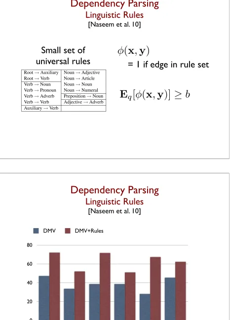
Posterior Sparsity
[Graça et al. 10]•
ML learns very ambiguous grammars
•
all productions have some probability
•
constrain the number of possible
productions
Dependency Parsing
Posterior Sparsity
[Gillenwater et al. 11] Measuring ambiguity on distributions over treesN → N V → N AD J → N N → V V → V AD J → V N → AD J V → AD J AD J → AD J
SparsityN is V
workingV 0.4
0.6 0 1 0
SparsityN is V
workingV 0.4
0.6 .4 .6 0
Use V good ADJ grammarsN 0.7
0.3 0 .7 .3
Use V good ADJ grammarsN 0.4 0.6
.4 .6 0
max↓
sum = 3.3← 0 1 .3 .4 .6 0 .4 .6 0
Dependency Parsing
Posterior Sparsity
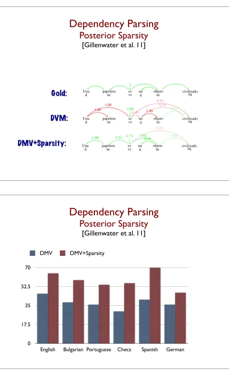
[Gillenwater et al. 11]GILLENWATER, GANCHEV, GRAÇA, PEREIRA, TASKAR
Una
d papeleranc esvs und objetonc civilizadoaq
Una
d papeleranc esvs und objetonc civilizadoaq
1.00 1.00 1.00 0.49 0.51 1.00 0.57 0.43 Una
d papeleranc esvs und objetonc civilizadoaq
1.00 0.83 0.75 0.920.99
0.35
[image:43.612.78.537.19.766.2]0.48
Figure 14: Posterior edge probabilities for an example sentence from the Spanish test corpus. Top
is Gold,middleis EM, andbottomis PR.
since then it does not have to pay the cost of assigning a parent with a new tag to cover each noun that does not come with a determiner.
Table 4 contrasts the most frequent types of errors EM, SDP, and PR make on several test sets where PR does well. The “acc” column is accuracy and the “errs” column is the absolute number
of errors of the key type. Accuracy for the key “parent POS truth/guess→child POS” is computed
as a function of the true relation. So, if the key ispt/pg →c, then accuracy is:
acc= # ofpt→cin Viterbi parses
# ofpt→cin gold parses . (25)
In the following subsections we provide some analysis of the results from Table 4.
7.1 English Corrections
Considering English first, there are several notable differences between EM and PR errors. Similar to the example for Spanish, the direction of the noun-determiner relation is corrected by PR. This is
reflected by the VB/DT→NN key, the NN/VBZ→DT key, the NN/IN→DT key, the IN/DT→
NN key, the NN/VBD→DT key, the NN/VBP→DT key, and the NN/VB→DT key, which for
EM and SDP have accuracy 0. PR corrects these errors.
A second correction PR makes is reflected in the VB/TO→VB key. One explanation for the
reason PR is able to correctly identify VBs as the parents of other VBs instead of mistakenly making TO the parent of VBs is that “VB CC VB” is a frequently occurring sequence. For example, “build and hold” and “panic and bail” are two instances of the “VB CC VB” pattern from the test corpus. Presented with such scenarios, where there is no TO present to be the parent of VB, PR chooses the first VB as the parent of the second. It maintains this preference for making the first VB a parent of the second when encountered with “VB TO VB” sequences, such as “used to eliminate”, because it would have to pay an additional penalty to make TO the parent of the second VB. In this manner,
PR corrects the VB/TO→VB key error of EM and SDP.
26 Gold: DVM: DMV+Sparsity:
Dependency Parsing
Posterior Sparsity
[Gillenwater et al. 11]0 17.5 35 52.5 70
English Bulgarian Portuguese Checz Spanish German
Dependency Parsing
Linguistic Rules
[Naseem et al. 10]Using Universal Linguistic Knowledge to Guide Grammar Induction
Tahira Naseem, Harr Chen, Regina Barzilay
Computer Science and Artificial Intelligence Laboratory Massachusetts Institute of Technology
{tahira, harr, regina} @csail.mit.edu
Mark Johnson
Department of Computing Macquarie University
Abstract
We present an approach to grammar induc-tion that utilizes syntactic universals to im-prove dependency parsing across a range of languages. Our method uses a single set of manually-specified language-independent rules that identify syntactic dependencies be-tween pairs of syntactic categories that com-monly occur across languages. During infer-ence of the probabilistic model, we use pos-terior expectation constraints to require that a minimum proportion of the dependencies we infer be instances of these rules. We also auto-matically refine the syntactic categories given in our coarsely tagged input. Across six lan-guages our approach outperforms state-of-the-art unsupervised methods by a significant mar-gin.1
1 Introduction
Despite surface differences, human languages ex-hibit striking similarities in many fundamental as-pects of syntactic structure. These structural corre-spondences, referred to assyntactic universals, have been extensively studied in linguistics (Baker, 2001; Carnie, 2002; White, 2003; Newmeyer, 2005) and underlie many approaches in multilingual parsing. In fact, much recent work has demonstrated that learning cross-lingual correspondences from cor-pus data greatly reduces the ambiguity inherent in syntactic analysis (Kuhn, 2004; Burkett and Klein, 2008; Cohen and Smith, 2009a; Snyder et al., 2009; Berg-Kirkpatrick and Klein, 2010).
1The source code for the work presented in this paper is
available at http://groups.csail.mit.edu/rbg/code/dependency/
[image:44.612.74.540.60.708.2]Root→Auxiliary Noun→Adjective Root→Verb Noun→Article Verb→Noun Noun→Noun Verb→Pronoun Noun→Numeral Verb→Adverb Preposition→Noun Verb→Verb Adjective→Adverb Auxiliary→Verb
Table 1: The manually-specified universal dependency rules used in our experiments. These rules specify head-dependent relationships between coarse (i.e., unsplit) syntactic categories. An explanation of the ruleset is pro-vided in Section 5.
In this paper, we present an alternative gram-mar induction approach that exploits these struc-tural correspondences by declaratively encoding a small set of universal dependency rules. As input to the model, we assume a corpus annotated with coarse syntactic categories (i.e., high-level part-of-speech tags) and a set of universal rules defined over these categories, such as those in Table 1. These rules incorporate the definitional properties of syn-tactic categories in terms of their interdependencies and thus are universal across languages. They can potentially help disambiguate structural ambiguities that are difficult to learn from data alone — for example, our rules prefer analyses in which verbs are dependents of auxiliaries, even though analyz-ing auxiliaries as dependents of verbs is also consis-tent with the data. Leveraging these universal rules has the potential to improve parsing performance for a large number of human languages; this is par-ticularly relevant to the processing of low-resource
Small set of
universal rules
= 1 if edge in rule set
E
q[φ(
x
,
y
)]
≥
b
φ
(
x
,
y
)
Dependency Parsing
Linguistic Rules
[Naseem et al. 10]0 20 40 60 80
English Danish Portuguese Slovene Spanish Swedish
Dependency Parsing:
Applications using Other Models
•
Tree CRF
•
[Druck et al. 09]•
MST Parser
•
[Ganchev et al. 09]Other Applications
•
Multi view learning:
•
[Ganchev et al. 08]•
Relation extraction:
Implementation Tips and Tricks
Off-the-Shelf Tools: MALLET
http://mallet.cs.umass.edu
•
off-the-shelf support for labeled features•
models: MaxEnt Classifier, Linear Chain CRF (one and two label constraints)•
methods: GE and PR•
constraintson label distributions for input features•
GE penalties: KL divergence, (+ soft inequalities)•
PR penalties: (+ soft inequalities)•
in development:Tree CRF, and other penalties�22
�22
Off-the-Shelf Tools: MALLET
http://mallet.cs.umass.edu
•
import data in SVMLight-like or CoNLL03-like formats•
import constraints in a simple text format:•
easily specify method options (i.e. SimpleTagger):positive interesting:2 film:1 ... negative tired:1 sequel:1 ... positive best:1 recommend:2 ...
U.N. NNP B-NP B-ORG official NN I-NP O heads VBZ B-VP O
tired negative:0.8 positive:0.2 best positive:0.9 negative:0.1
U.N. B-ORG:0.7,0.9 B-VP O:0.95,
java cc.mallet.fst.semi_supervised.tui.SemiSupSimpleTagger \ --train true --test lab --loss l2 --learning ge \
unlabeled.txt test.txt constraints.txt
New GE Constraints: MALLET
http://mallet.cs.umass.edu
•
Java Interfaces for implementing new GE constraints•
covariance computation implemented (MaxEnt, CRF)•
primarily need to write methods to:•
restriction:constraints must factor with model•
restriction:GE objective must be differentiablecompute constraint features and expectations compute GE objective value
New PR Constraints: MALLET
http://mallet.cs.umass.edu
•
Java Interfaces for implementing new PR constraints•
inference algorithms implemented (MaxEnt, CRF)•
primarily need to write methods for E-step (projection):•
restriction: constraints must factor with modelcompute constraint features and expectations compute scores under q for E-step
compute objective function for E-step compute gradient for E-step
GE Implementation Advice
•
computing covariance (required for gradient):•
trick: compute cov. of composite constraint feature•
example: penalty:•
result: only need to store vectors of size in computation, rather than covariance matrix•
trick: efficient gradient computation in hypergraphs•
use semiring algorithms of [Li & Eisner 09]•
result: same time complexity as supervised (w. both) φc(x,y) =�
φ
2( ˜φ−E[φ])φ(x,y)
�22
GE Implementation Advice
•
parameter regularization:•
regularization encourages bootstrapping by penalizing very large parameter values:•
optimization: non-convex•
usually L-BFGS still preferable (use “restart trick”)•
zero initialization usually works well•
other init: supervised, MaxEnt, GE in simpler model�22
>
Off-the-Shelf Tools: PR Toolkit
http://code.google.com/p/pr-toolkit/
•
off-the-shelf support for PR•
models:•
MaxEnt Classifier, HMM,DMV•
applications:•
Word Alignment, Pos Induction, Grammar Induction•
constraints:posterior sparsity, bijectivity, agreement•
No command line modePR Implementation example:
Word Alignment - Bijectivity
•
Learning:EM, PR• void eStep(counts, lattices);
• void mStep(counts);
• lattice constraint.project(lattice);
•
Model:HMM• lattice computePosteriors(lattice);
• void addCount(lattice, counts);
• void updateParameters(counts);
•
Constraints: Bijectivity• lattice project(lattice);
PR Implementation example:
EM
class EM {
model;
void em(n){
lattices= model.getLattices(); counts = model.counts();
for(i=0; i< n; i++) {
eStep(counts, lattices); mStep(counts);
} }
void eStep(counts, lattices) {
counts.clear();
for(l : lattices) {
model.computePosterior(l); model.addCount(l,counts); }
}
void mStep(counts) {
model.updateParameters(counts); }
...
PR Implementation example:
PR
class PR {
model;
constraint;
void em(n){
lattices= model.getLattices(); counts = model.counts();
for(i=0; i< n; i++) {
eStep(counts, lattices); mStep(counts);
} }
void eStep(counts, lattices) {
counts.clear();
for(l : lattices){
model.computePosterior(l); constraint.project(l);
model.addCount(l,counts); }
}
void mStep(counts) {
model.updateParameters(counts); }
...
}
PR Implementation example:
HMM
class HMM {
obsProb, transProbs,initProbs;
lattice computerPosteriors(lattice){ “Run forward backward”
}
void addCount(lattice,counts){
“Add posteriors to count table” }
void updateParams(counts){
“Normalize counts”
“Copy counts to params table” }
void getCounts(){
“return copy of params structures” }
void getLattices(){
“return structure of all lattices in the corpus”
}
...
PR Implementation example:
Bijective constraints
•
Constraint: returns a vector with mth value = number of target words in sentence x that align with source word mφ(x,y) =
N
�
i=1
1(yi =m) Q = {q : Eq[φ(x,y)] ≤ 1}
•
Primal:HardDKL(Q|pθ) = arg min
q DKL(q|pθ)
•
Dual:Easyarg max
λ≥0 −
bT ·λ−logZ(λ)−||λ||2
Z(λ) = �
y
pθ(y|x) exp(−λ·φ(x,y))
PR Implementation example:
Bijective Constraints
class BijectiveConstraints {
model;
lattice project(lattice){
obj = BijectiveObj(model,lattice); Optimizer.optimize(obj);
}
}
class BijectiveObj { lattice;
void updateModel(newLambda){
lattice_ = lattice*exp(newLambda); computerPosteriors(lattice)
}
double getObj(){
obj = -dot(lambda,b); obj -= lattice.likelihood; obj -= l2Norm(lambda); }
double[] getGrad(){
grad = lattice.posteriors - b; grad -= norm(lambda);
Other Software Packages
•
Learning Based Java:•
http://cogcomp.cs.illinois.edu/page/software_view/11•
support for Constraint-Driven Learning•
Factorie:Rich Prior Knowledge in Learning for Natural
Language Processing
Bibliography
For a more up-to-date bibliography as well as additional information about these methods, point your browser to: http://sideinfo.wikkii.com/
1 Constraint-Driven Learning
Constraint driven learning (CoDL) was first introduced in Chang et al. [2007], and has been used also in Chang et al. [2008]. A further paper on the topic is in submission [Chang et al., 2010].
2 Generalized Expectation
Generalized Expectation (GE) constraints were first introduced by Mann and McCallum [2007]1and were used to incorporate prior knowledge about the label
distribution into semi-supervised classification. GE constraints have also been used to leverage “labeled features” in document classification [Druck et al., 2008] and information extraction [Mann and McCallum, 2008, Druck et al., 2009b, Bellare and McCallum, 2009], and to incorporate linguistic prior knowledge into dependency grammar induction [Druck et al., 2009a].
3 Posterior Regularization
The most clearly written overview of Posterior Regularization (PR) is Ganchev et al. [2010]. PR was first introduced in Graca et al. [2008], and has been applied to dependency grammar induction [Ganchev et al., 2009, Gillenwater et al., 2009, 2011, Naseem et al., 2010], part of speech induction [Gra¸ca et al., 2009a], multi-view learning [Ganchev et al., 2008], word alignment [Graca et al., 2008, Ganchev et al., 2009, Gra¸ca et al., 2009b], and cross-lingual semantic alignment [Platt et al., 2010]. The framework was independently discovered by Bellare et al. [2009] as an approximation to GE constraints, under the name Alternating Projections, and used under that name also by Singh et al. [2010] and Druck and McCallum [2010] for information extraction. The framework was also independently discovered by Liang et al. [2009] as an approximation to
a Bayesian model motivated by modeling prior information as measurements, and applied to information extraction.
4 Closely related frameworks
Quadrianto et al. [2009] introduce a distribution matching framework very closely related to GE constraints, with the idea that the model should pre-dict the same feature expectations on labeled and undlabeled data for a set of features, formalized as a kernel.
Carlson et al. [2010] introduce a framework for semi-supervised learning based on constraints, and trained with an iterative update algorithm very similar to CoDL, but introducing only confident constraints as the algorithm progresses. Gupta and Sarawagi [2011] introduce a framework for agreement that is closely related to the PR-based work in Ganchev et al. [2008], with a slightly different objective and a different training algorithm.
References
K. Bellare, G. Druck, and A. McCallum. Alternating projections for learning with expectation constraints. InProc. UAI, 2009.
Kedar Bellare and Andrew McCallum. Generalized expectation criteria for boot-strapping extractors using record-text alignment. InEMNLP, pages 131–140, 2009.
Andrew Carlson, Justin Betteridge, Richard C. Wang, Estevam R. Hruschka Jr., and Tom M. Mitchell. Coupled Semi-Supervised Learning for Information Extraction. In Proceedings of the Third ACM International Conference on Web Search and Data Mining (WSDM), 2010.
M. Chang, L. Ratinov, and D. Roth. Guiding semi-supervision with constraint-driven learning. InProc. ACL, 2007.
Ming-Wei Chang, Lev Ratinov, and Dan Roth. Structured learning with con-strained conditional models. 2010. In submission.
M.W. Chang, L. Ratinov, N. Rizzolo, and D. Roth. Learning and inference with constraints. In Proceedings of the National Conference on Artificial Intelligence (AAAI). AAAI, 2008.
G. Druck, G. Mann, and A. McCallum. Learning from labeled features using generalized expectation criteria. InProc. SIGIR, 2008.
Gregory Druck and Andrew McCallum. High-performance semi-supervised learning using discriminatively constrained generative models. InProceedings of the International Conference on Machine Learning (ICML 2010), pages 319–326, 2010.
Gregory Druck, Burr Settles, and Andrew McCallum. Active learning by label-ing features. InEMNLP, pages 81–90, 2009b.
K. Ganchev, J. Gra¸ca, J. Blitzer, and B. Taskar. Multi-view learning over structured and non-identical outputs. InProc. UAI, 2008.
K. Ganchev, J. Gillenwater, and B. Taskar. Dependency grammar induction via bitext projection constraints. InProc. ACL-IJCNLP, 2009.
Kuzman Ganchev, Joo Graa, Jennifer Gillenwater, and Ben Taskar. Posterior sparsity in unsupervised dependency parsing. Journal of Machine Learn-ing Research, 11:2001–2049, July 2010. URLhttp://jmlr.csail.mit.edu/ papers/v11/ganchev10a.html.
Jennifer Gillenwater, Kuzman Ganchev, Joo Graa, Ben Taskar, and Fernando Pereira. Sparsity in grammar induction. In NIPS Workshop on Grammar Induction, Representation of Language and Language Learning, 2009.
Jennifer Gillenwater, Kuzman Ganchev, Joo Graa, Fernando Pereira, and Ben Taskar. Posterior sparsity in unsupervised dependency parsing. Journal of Machine Learning Research, 12:455–490, February 2011. URLhttp://jmlr. csail.mit.edu/papers/v12/gillenwater11a.html.
Joao Graca, Kuzman Ganchev, and Ben Taskar. Expectation maximization and posterior constraints. In J.C. Platt, D. Koller, Y. Singer, and S. Roweis, editors, Advances in Neural Information Processing Systems 20, pages 569– 576. MIT Press, Cambridge, MA, 2008.
J. Gra¸ca, K. Ganchev, F. Pereira, and B. Taskar. Parameter vs. posterior sparisty in latent variable models. InProc. NIPS, 2009a.
J. Gra¸ca, K. Ganchev, and B. Taskar. Postcat - posterior constrained alignment toolkit. InThe Third Machine Translation Marathon, 2009b.
Rahul Gupta and Sunita Sarawagi. Joint training for open-domain extraction on the web: exploiting overlap when supervision is limited. InProceedings of the Fourth ACM International Conference on Web Search and Data Mining (WSDM), 2011.
P. Liang, M. I. Jordan, and D. Klein. Learning from measurements in exponen-tial families. InProc. ICML, 2009.
G. S. Mann and A. McCallum. Generalized expectation criteria for semi-supervised learning of conditional random fields. InProc. ACL, 2008.
Tahira Naseem, Harr Chen, Regina Barzilay, and Mark Johnson. Using uni-versal linguistic knowledge to guide grammar induction. In Proceedings of the 2010 Conference on Empirical Methods in Natural Language Processing, pages 1234–1244, Cambridge, MA, October 2010. Association for Computa-tional Linguistics. URLhttp://www.aclweb.org/anthology/D10-1120. John Platt, Kristina Toutanova, and Wen-tau Yih. Translingual document
rep-resentations from
![Figure 4.1: The model used by Liang et al. [2009], using our notation. We have separatedObjective: mode of given observationsθ](https://thumb-us.123doks.com/thumbv2/123dok_us/227478.522136/22.612.74.540.54.772/figure-model-liang-using-notation-separatedobjective-given-observationsth.webp)