One parameter model of sterilisation process Heating and cooling period

One-parameter model of sterilisation process. Heating

and cooling period

M. Loučka, P. Veselý, F. Jaroš, J. Pavlík

Department of Mathematics, Faculty of Chemical Engineering, Institute of Chemical

Technology, Prague, Czech Republic

Abstract: The article deals with the simplification of the heat transfer model for food sterilisation in cans and jars. The one-parameter model was derived and identification procedures of its parameters were examined. It is shown that the concept of the first order dynamics satisfies the technological purposes but the common method of the least squares is not suitable for the calculation of model constants. A new computing method is presented and compared with statisti-cally evaluated experiments with wide range of stuffs and packages.

Keywords: sterilisation effect; thermal treating of foods; temperature profile; parameters evaluation; first order dynam-ics; preservation of foods; thermal processing

Technological requirements for heat treatment of foods need generaly the fulfillment of two con-ditions: first - it is necessary to reach a given tem-perature in a given geometric point; second - this temperature has to be maintained during a given time period. The temperature regime is determined by the regular value of F-effect defined by the for-mula

(1)

The fulfillment of analogical conditions is also required when other thermal operations are per-formed - cooking, roasting, smoking and even freez-ing, when solid or packed foods are processed.

Works concerning this engineering problem (Stumbo 1973; Leninger & Beverloo 1975; Loučka & Klein 1985) use the simplified classi-cal Fourier-Kirchhoff equations for long duration processes and they derive from the linear part of the logarithmic transformed temperature curve the empirical f and j factors, with the help of which the temperature curve can be predicted in similar cases. Many works in this field are based on this concept (Hayakawa 1977) and give satisfactory results in comparison with the numerical solution of the Fou-rier-Kirchhoff equations. Particularly the simplicity of the idea of f and j factors is the reason, why this method may be a starting point of more sofisticated considerations on the dynamics of sterilisation heat

transfer processes. Analogical characteristic was introduced (Videv & Tančev 1986) that a priori considers the heat transfer to a sterilized can to be a lumped parameter system with the dynamics of the first order. Unlike the above mentioned method, the Videv’s time constant does not depend on the course of the time temperature curve in the sterili-sation medium.

On the base of Stumbo and Ball-Ohlson theory there were designed computer programs for com-puting the sterilisation process parameters (Haya- kawa 1977). On the other hand, in some papers (Pečová et al. 1984), the nonparametric methods are used for the same purpose.

MATERIAL AND METHODS

Theory

In some works (Loučka & Kutal 1983; McKen- na & Holdsworth 1991) the mass transfer equa-tion for a cylindrical body supposing the thermal diffussivity being constant with the boundary conditions of the first or third kind is solved by the application of the Duhamell theorem. With the help of it there was derived a relation between the time-temperature course on the surface or in the neighbourhood of a body and in its geometric midpoint. By the way of generalization a lumped parameters model was costructed in which there

0

( )

10

z

t

F t

dt

³

appear no physical properties of the body except quantities that are possible to be determined by methods of experimental identification. The model is described by the following equations (Himmel-blau & Bischoff 1968):

0

( ) ( , ). ( )

t

Y t = ∫H t −τ P X τ dt (2)

The function H (τ, →P) is an impulse characteristic. Its explicite form can be found by the method of model transfer function known in the theory of regulation. The system is then described by an ordi-nary differential equation the order of which equals to the dimension of the vector of parameters:

(3)

The above explained procedure is not new and many former works follow this concept (Skinner 1984; Loučka & Klein 1985). Nevertheless, they differ in the recommended order of the system. In some papers (Loučka & Klein 1985; Videv & Tančev 1986) there is recommended the system of the first order, where H(τ, →P) is a solution of the equation

( , ) ( , ) . ( )

H t P′  +αH t P =α δ t (4)

with the condition

H(0, →P) = 0 (5)

while Skinner found the best agreement with the reality for the system of the fifth order.

Experimental

Identification of a dynamic system is a task that includes the measuring and monitoring of the time course input and output quantities and consequent evaluation of parameters and order of the system (see equation (3)). The output calculated from this equation ought to agree closely with the experi-mental data in accordance with the criterion set in advance.

The experiments were characterized by the sim-plicity of its technical arrangement. From two as minimum to sixteen as maximum temperature courses were measured and monitored. The input signals were chosen initially as a temperatue step change, later as a general pulse.

The step signal was realized by the laboratory equipment, which was composed from two vessels of different temperature and thermal capacity which were many times higher than those of the examined can. The cans were brought from one vessel over to the other. At first the step signal was supposed to be ideal and only the response – the temperature in each can was measured. In the case of the gen-eral input both the impulse and the response were measured and evaluated. The temperatures were measured by thermocouples and monitored in the time interval of 30 s by a data acquisition computer. The accuracy of measurement was guaranteed in the range of 20–120°C ± 0.1°C. The data were filtered with regard to any systematic errors as well as to the higher frequency noise. All realized experiments along with their results are presented in (8).

Evaluation of parameters

The obtained data were used for the following purposes:

(1) the confirmation of the hypothesis about validity of the first order dynamics;

(2) the verification of the fact that the parameters used for modelling the heating as well as the cooling period coincide;

(3) choice of a method of the identification of the parameters suitable for practical use.

In order to solve the problems (1) and (2) the sets of data represented by the records of responses to the step temperature change were used. On the basis of these results the data corresponding to the real courses of the bath and can temperature during the sterilisation were treated as responses to a general signal for the solution of the problem (3).

Mathematical formulation of the first problem is based on the fact that when the model of the first and second order dynamics is used, the hypothesis of the statistical equality of residual sum of squares can be accepted. The criterion used

Φ = S1 (r – 2) ₍₆₎

S2 (r – 1)

has the Snedecore distribution with the critical value F(r – 2), (r – 1), β. The critical domain of the test

(at the 1 – β level of significance with r – 1 and r – 2 degree of freedom) is given by:

P(Φ > Φ (r – 2), (r – 1), β)= β (7)

S₁ and S₂ are residual sums of squares of deviations from the theoretical curve given by the solution of

( ) ( 1) ( )

1 1 0 0

n n m

a Y_n a Y_n a Y a Y b Xc _m b X

( ) ( 1) ( )

1 1 0 0

n n m

the equation (3) for n = 1 and n = 2 respectively. In both cases there is X = 1 and m = 0. There are obtained the known formulas for dynamic response of a system of the first and second order on the step input (see (14)). The parameters of the models are consequently calculated by the method of the least squares principle. For the system of the first order there holds the equation

(8)

while for the system of the second order there holds the following one:

(9)

In case it is statistically proved e.g. on the basis of the criterion (6) that the consent of the model and the experiment does not improve when the model order increases, it would make no sense to consider a model with a higher number of parameters.

However, if the one-parameter model is consid-ered, there appears a new question about whether the values of the constants α_H and α_C for heating and cooling period are the same, because there may occur irreversible changes of a can content during the thermal treatment. Both constants α_H and α_C depend above all on the thermodynamical and rheological properties of the content of a can. In addition to it, they could change depending on the packing and on the conditions of the convection concerning the heating media. They have different values both in the stationary and the rotation retort, the difference being greater the more the convection participates in the inner heat transfer.

While the statistical distribution of estimated val-ues α is not generally normal, the non-parametric signum test (Freund & Walpole 1980) was used that compares two random choices from the same population of a not necessarily known distibution. There were calculated differences between the cou-pled values from a sample of the size r:

d_i= x_i – y_i, i = 1, …, r (10)

The null hypothesis supposes medians of both the samples being equal. Let us denote R₊ and R_– the numbers of the positive or the negative differences respectively and R₀ the number of differences equal to zero. Let us put

r₀ = R₊, r₁ = r –R₀ (11)

For a reliability level β chosen in advance the criti-cal values q₁(r₁) and q₂(r₁) for r < 20 are tabulated. The critical domain is given by the inequalities

r₀ < q₁(r₁) and r₀> q₂(r₁) (12)

When these conditions are fulfilled, the null hypothesis is rejected and the alternative one is accepted.

Identification of parameters in the general input

From the point of view of mathematics the prob-lem means to minimize the function

(13)

on the conditions the validity of the model of the first order according to equations (7), (8) and (9) is guaranteed. Numerical solution of one non-linear equation

(14)

gives reliable results. However, this conception of the criterion does not give satisfying results for the calculation of the F-value. The reason is, as it was already mentioned, that the most significant influ-ence on the value of the integral (1) has that part of the temperature curve, where the temperature of the contents of the can is very close to the reference temperature T_r.

This fact was taken into account when the values of the parameter α from responses to the step change were calculated. The method of weighted regression was used, the criterion having the form

(15)

In order the condition to be fulfilled that the weight functions have the highest values for the highest temperatures T_k they were chosen as in-creasing functions of the temperature with a con-stant s set in a suitable way:

W₁(t) = sT_exp(t), W₂(t) = sT 2

exp(t), W3(t) = esTexp(t) (16)

If F_mod are the values of the integral (1), calculated from the equation (2) with the corresponding pa-rameter and F_exp the value of sterilisation effect for an experimental course T_exp(t), then the function

(17)

1 exp

2

( ) ( ( ) 1 ) ,

1 i

ti n

G Y t e

i

D

D ¦

2 1

1 2

1 1 2 _exp

1 2

2

( , ) ( ) 1 .

1

i i

i

t t

n e e

G Y t

i Z Z Z Z Z Z Z Z ¦

§

·

¨

¸

¨

¸

©

¹

2 ( ) ( ( ) ( , ) ( ) ) 1 0 i i i t n

G Y t H t X d

i

D ¦ ³ W D W W

01( )

0 dG d D D 1 exp 2

( ) ( )( ( ) 1 ) ,

1 i i

ti

n

G W t T t e

reaches its minimal value at the point α_F, which is consistent with the requirement of agreement of the sterilisation effect. From the point of view of the microbiological quality the temperature profiles measured experimentally and calculated from the model have minimal differences.

RESULTS

The wide range of cans with different kinds of fill-ing and package were subject of the experimental observation.

The description of all experimental circumstances is presented in detail in the Table 5 along with the results of the evaluation of experiments. That means the determination of dynamics system order both for the heating and for the cooling period and the evaluation of the signum tests for the decision con-cerning differences between dynamic constant α for heating and cooling periods.

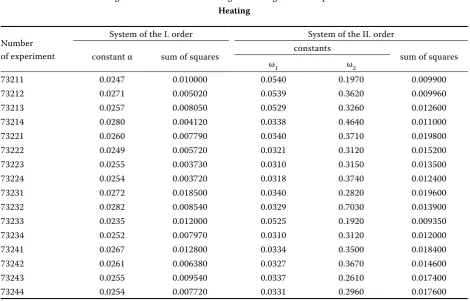
The Tables 1 and 2 describe the behaviour of a can (filled with Luncheon meat) which underwent step temperature change from 25–85°C. There was observed the dynamics of the first order as well as the agreement of constants α_H and α_C . The

evalu-ation was performed by the non-linear regression method and the criterions given by equations (8) and (9) were used. The results of another experiment having the same behaviour are in the Tables 3–4, when filling of the 500 g can was pea. The can was treated by the step temperature change and there was also confirmed the dynamics of the first order by the Snedecore test.

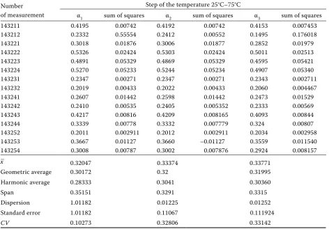
The results of the weighted regression using the criterion (17) are presented in the Table 4. Three different weight functions given by equations (18) were used consecutively. It can be seen in the sec-ond, fourth and sixth column of this table that the constants α_i calculated by this method differ very little and that they are in agreement with the con-stant α obtained by the use of the criterion (8) (to compare with the second column of the Table 3.). The similar agreement of results of the ordinary and weighted regression was observed in all cases. The Table 5. demonstrates that in most experiments just like those described in the Tables 1–4 the heating or cooling of a can have the first order dynamics. The results of the signum test that should evaluate the consent of the constants α for heating and cooling periods of sterilisation show another behaviour: the

Table 1. The example of the statistical test (Willcoxon’s test) for setting out the order of the heating process dynamics (see the third and the sixth columns of the table)

Filling: Luncheon meat Packeage: can 500 g Step: 25°C–85°C

Heating

Number of experiment

System of the I. order System of the II. order

constant α sum of squares constants sum of squares

ω₁ ω₂

73211 0.0247 0.010000 0.0540 0.1970 0.009900

73212 0.0271 0.005020 0.0539 0.3620 0.009960

73213 0.0257 0.008050 0.0529 0.3260 0.012600

73214 0.0280 0.004120 0.0338 0.4640 0.011000

73221 0.0260 0.007790 0.0340 0.3710 0.019800

73222 0.0249 0.005720 0.0321 0.3120 0.015200

73223 0.0255 0.003730 0.0310 0.3150 0.013500

73224 0.0254 0.003720 0.0318 0.3740 0.012400

73231 0.0272 0.018500 0.0340 0.2820 0.019600

73232 0.0282 0.008540 0.0329 0.7030 0.013900

73233 0.0235 0.012000 0.0525 0.1920 0.009350

73234 0.0252 0.007970 0.0310 0.3120 0.012000

73241 0.0267 0.012800 0.0334 0.3500 0.018400

73242 0.0261 0.006380 0.0327 0.3670 0.014600

73243 0.0255 0.009540 0.0337 0.2610 0.017400

73244 0.0254 0.007720 0.0331 0.2960 0.017600

values of these constants are significantly different in several cases (see Table 5).

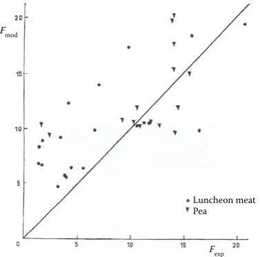
The most important criterion of sterilisation process control remains to be the F-value. Each procedure for the determination of any constants is justified only when it leads to the knowledge of this quantity with satisfactory precision. The F -val-ues were calculated with the use of the constant α obtained by the evaluation of experimental data. They were substituted to the equation (2) and com-pared with those which were calculated from the real experimental courses. The results obtained by both methods differ significantly (see Figure 1). That confirms the fact that there does not exist a simple way how to use the model constants determined by the standard regression method for description and prediction of a real process. The agreement of the sterilisation trajectories calculated in various ways is presented in the Figure 2. It is clear that there are

no great differences between these curves from the point of view of a qualitative similarity.

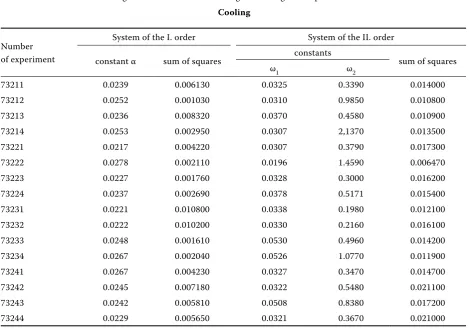
However, because the sterilisation effect (F-value) is most sensible with regard to that part of tempera-ture trajectory where the maximum is achieved, the standard regression methods fall down. That is why an algorithm for the determination of the constant α was developed that uses the criterion given by equation (17). In the Figure 3 there are shown the courses of the identification problem solution for two different cans made both by the standard re-gression method (continuous line) and developed algorithm procedure (dashed line). In both cases, the final results differ and the course describing the dependence between the value of the criterion and the constant α has always a distinguishable mini-mum value. From Figure 2 there can be seen that the agreement between the experimental curve and the curve calculated with the help of the criterion (17) Table 2. (1) The example of the statistical test (Willcoxon’s test) for setting ou the order of the cooling process dynamics (see the third and the sixth columns of the table); (2) The sign test(Willcoxon’s test) of agreement of alpha-constant from the Table 1 and the Table 2. It is to compare that for the heating as well as for the cooling period the same value alpha can be used

Filling: Luncheon meat Package: can 500 g Step: 85°C–25°C

Cooling

Number of experiment

System of the I. order System of the II. order

constant α sum of squares constants sum of squares

ω₁ ω₂

73211 0.0239 0.006130 0.0325 0.3390 0.014000

73212 0.0252 0.001030 0.0310 0.9850 0.010800

73213 0.0236 0.008320 0.0370 0.4580 0.010900

73214 0.0253 0.002950 0.0307 2,1370 0.013500

73221 0.0217 0.004220 0.0307 0.3790 0.017300

73222 0.0278 0.002110 0.0196 1.4590 0.006470

73223 0.0227 0.001760 0.0328 0.3000 0.016200

73224 0.0237 0.002690 0.0378 0.5171 0.015400

73231 0.0221 0.010800 0.0338 0.1980 0.012100

73232 0.0222 0.010200 0.0330 0.2160 0.016100

73233 0.0248 0.001610 0.0530 0.4960 0.014200

73234 0.0267 0.002040 0.0526 1.0770 0.011900

73241 0.0267 0.004230 0.0327 0.3470 0.014700

73242 0.0245 0.007180 0.0322 0.5480 0.021100

73243 0.0242 0.005810 0.0508 0.8380 0.017200

73244 0.0229 0.005650 0.0321 0.3670 0.021000

Dynamics of the first order

The result of the accomplished sign test: P = 0.035156

Table 3. The verification of the order of dynamics for another sort of food (pea)

Filling: Sterilized Green Peas Package: can 500 g Step: 25°C–75°C

Heating

Number of experiment

System of the I. order System of the II. order

constant α sum of squares constants sum of squares

ω₁ ω₂

143211 0.4195 0.00742 0.826574 0.82451 0.003762

143212 0.2332 0.5555 0.543216 0.54244 0.025054

143221 0.3018 0.01876 0.602344 0.60210 0.006996

143222 0.5326 0.02424 1.010310 1.01545 0.007279

143223 0.4891 0.05329 0.866366 0.86423 0.011179

143224 0.5270 0.05233 0.968369 0.97098 0.011198

143231 0.2347 0.00271 0.510141 0.50909 0.002912

143232 0.2019 0.00433 0.446285 0.44626 0.001872

143241 0.2607 0.01442 0.530169 0.52748 0.006399

143242 0.2410 0.00535 0.507826 0.50783 0.004607

143243 0.4217 0.00816 0.814009 0.81467 0.005107

143244 0.3339 0.00778 0.656725 0.65556 0.005183

143253 0.3667 0.01127 0.694231 0.69338 0.006167

143254 0.3008 0.00787 0.619143 0.62076 0.004450

Dynamics of the first order, P < 0.05

Table 4. Results of the weighted regression Using the weighted regression with the weight functions w₁,w₂,w₃ respectively for counting the constants α₁,α₂,α₃ .

Number of measurement

Step of the temperature 25°C–75°C

α₁ sum of squares α₂ sum of squares α₃ sum of squares

143211 0.4195 0.00742 0.4192 0.00742 0.4153 0.007453

143212 0.2332 0.55554 0.2412 0.00552 0.1495 0.176018

143221 0.3018 0.01876 0.3006 0.01877 0.2852 0.01979

143222 0.5326 0.02424 0.5303 0.02424 0.5011 0.02513

143223 0.4891 0.05329 0.4869 0.05329 0.4595 0.05421

143224 0.5270 0.05233 0.5244 0.05234 0.4907 0.05340

143231 0.2347 0.00271 0.2347 0.00271 0.2343 0.002711

143232 0.2019 0.00433 0.2022 0.00433 0.2060 0.004467

143241 0.2607 0.01442 0.2598 0.01442 0.2473 0.01529

143242 0.2410 0.00535 0.2405 0.005352 0.2333 0.00569

143243 0.4217 0.00816 0.4209 0.008165 0.4093 0.00844

143244 0.3339 0.00778 0.3332 0.007779 0.324 0.00807

143252 0.2011 0.002911 0.2012 0.002911 0.2034 0.002958

143253 0.3667 0.01127 0.3660 –0.01127 0.3559 0.011540

143254 0.3008 0.00787 0.3002 0.007876 0.2924 0.008157

–

x _{0.32047 0.33374 0.33771}

Geometric average 0.30172 0.32 0.31995

Harmonic average 0.28333 0.3041 0.30360

Span 0.35151 0.3291 0.3315

Dispersion 1.01182 0.01225 0.01252

Standard error 1.01182 0.11067 0.111924

CV 0.10273 0.32806 0.33142

When the values of the constants α₁,α₂,α₃ counted using the weighted regression with the weight functions w₁,w₂,w₃ respectively are compared it is evident that all the three ways give appreximately the same results

Table 5. Some experimental conditions and results

Filling Number of experiment Package Step Order of the system Sign test heating cooling

Country stew 521 S-460 25–65 II II I

522 S-460 25–85 I I I

Hungary stewt 622 S-460 25–85 II II I

731 P-500 25–65 I I I

Luncheon meat 732 P-500 25–85 I I I

832 P-500 25–85 I I I

VMVS 932 P-500 25–85 I I I

Meat cream 1041 P-80 25–65 I I I

Cabbage-S 1152 S 4/1 35–85 II II

Cabbage-D 1222 S-720 35–85 II II

Water

111 S-370 25–65 I I S

112 S-370 25–85 I I S

121 S-460 25–65 I I S

122 S-460 25–85 I I N

131 P-500 25–65 I I N

132 P-500 25–85 I I S

Beet

211 S-370 25–65 I I S

212 S-370 25–85 I I S

222 S-720 25–85 I I S

Pickles 311 S-370 25–65 II II S

321 S-370 25–85 I I N

Saussage with beens 421 S-460 25–65 II I S

422 S-460 25–85 II II S

P-value of the sign test and the Snedecore-Fisher test: P < 0.05

column “package”: S – jar, P – can, for example P-500 means a can with the filling of 500 gramm of stuff

column “sign test”: S – significant result of the sign test, zero hypothesis is rejected; N – nonsignificant results of the sign test, zero hypothesis can not be rejected

may not always be optimal in the sense of the least squares principle.

DISCUSSION

The experimental study of the thermal dynamic behaviour of one individual can or jar was com-pleted after experiments with five kinds of jars and two kinds of cans which were filled with fifteen kinds of real foodstuffs were performed and observed. A special attention was concentrated on the question of agreement of the F-value predicted from the model with its value determined from experimental data. For a wide range of the examined fillings there was confirmed that the process can be described by the first order dynamics model and that in many cases the same value of the constant α can be used Figure 1. The sterilization effect calculated from the model

(F_mod) and the experimental curve (F_exp) F_mod

F_exp

both for the increasing and the decreasing part of the sterilisation curve. However, the results of the calculated sterilisation effect differ when the real measured trajectory or the calculated trajectory of temperature is used. The practical use of the constants, calculated by the procedure, is therefore problematic. The reason of that is the fact that the

F-value depends mainly on the course of the steri-lisation curve near its maximum. In the prediction step the consent of heating and cooling parts of the curve is not so important, but it is significant during the temperature holding-up.

On the basis of this knowledge the criterion of data agreement was modified and the sterilisation

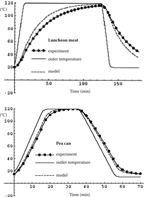
Figure 3. The comparison off the least squares method fitting (s-criterion) with the proposed method (phi-criterion) Figure 2. Examples of time-temperature courses in two different fillings with curve fitted by the model

Luncheon meat

experiment outer temperature

model

Pea can

experiment outlet temperature

model

Time (min)

Time (min) (°C)

(°C)

φ s

φ

s

φ

s

Pea can 0.5 kg 0.6 Luncheon meat 0.5 kg

0.5

0.4

0.3

0.2

0.1

0.7 0.6 0.5 0.4 0.3 0.2 0.1 0.08

0.06

0.04 0.03 0.02 0.01 0.4

0.3

0.2

0.1 ∑s_q

αφ = 0.0393

αs = 0.0308

∑s_q exp mod

exp

F F F

M exp mod

exp

F F F M

0.20 0.25 0.30 0.35 0.40

α (min–1₎

0.20 0.25 0.30 0.35 0.40

curve was substituted by the time-temperature course, which is not optimal in the common sense of the least squares of deviations but which is, with regard to the calculated F-value, in the best consent with the experimental curve. Then the method of weighted regression for the data obtained as a tem-perature step signal response was used with three different weight functions having their maximum value in the same range of the temperature as the ex-perimental curve. The method modified by this way turned out not to be satisfying and the treatment of the results by the step-response analysis despite of it significance for the understanding of the real process is not suitable for practical (e.g.industrial) implementation.

Despite the fact that for the dynamic constant α there holds the following expression

it is not possible to calculate its value from this formula. On the other side, this formula enables to consider the relations between this parameter and the quantities involved in the process. In addition to the rheological and thermophysical properties of the filling of a can the value of the constant α can be influenced by hydrodynamic relations, geometry of a can or a jar, the specific heat, weight and kind of the package. From this point of view the identi-fication experiment using a general input signal on an actual equipment seems to be the most suitable because it is in the best accordance with the real circumstances. The algorithm developed and tested in this paper may be used for such a purpose. It is based on the minimization criterion in the equation (17) and when used a very satisfactory agreement of F-values is reached.

If the parameters alpha identified for the whole range of production were known, two important problems could be solved. The first of them is the simple determination of the sterilisation effect F -value during the process on the basis of the bath temperature measuring. It is usually performed by the placement of the temperature sensor into the middle of the can, which may be in many cases difficult to realize not to mention the fact that it is always uncomfortable.

The second problem is more complicated and its technological significance is greater. The course of the temperature trajectory in the bath of the sterilisation unit is to be determined, especially the duration of the temperature holding-up and the residence time of cans in the cooling bath, when the

constant α and the F-value are known. An example of the solution of this problem was given in our previous paper (Loučka et al. 1987) with the ex-perimental confirmation of the proces prediction.

The values of constants for different products treated in preservation industry in Czech Repub-lic are summarized in our rewiev (Loučka et al. 1991).

Notation

A – area (m2₎

a_i, b_i – coefficients in the equation (3), constants c_P – heat capacity (J/kg/deg)

d – difference of the corresponding values in the signum test

F – sterilisation effect according to Ball-Ohlson (°C)

G – goal function of data fitting

H(τ, →P) – kernel function in a Volterra integral equation

k – total heat transfer coefficient (W/m2_/deg) M – mass (kg)

m – order of the input signal (see differential equation (3)

n – order of the output signal (see differential equation (3)

P – P-value, (the significance)

r – number of observations in statistical tests

→

P – vector of parameters

q – critical value of the sign test

S – summ of squares

T – temperature (°C)

t – time (sec)

W(t) – weight function

X(t) – general dynamic signal input

Y(t) – general dynamic signal output

z – slope of the thermoinactivation curve (°C)

Greek symbols

α – reciprocal value of the time constant (s–1₎

β – risk level in a statistical test 1 – β – significance level of a statistical test δ(t) – Dirac’s distribution

ω – parameters of the model of the second order (s–1₎

Ф – testing statistics of the Fischers’s test φ – criterion given by the equation (17)

Indices

C – cooling period H – heating period

mod – value, computed from the model exp – experimental value

r – reference value .

, . k A M c p

Abstrakt

Loučka M., Veselý P., Jaroš F., Pavlík J. (2006): Jednoparametrový model sterilačního procesu. Zahřívací a chladicí fáze. Res. Agr. Eng., 52: 97–106.

Práce se zabývá zjednodušením modelu přestupu tepla při sterilaci potravin v plechových nebo skleněných obalech. Byl odvozen jednoparametrový model a ověřen postup jeho identifikace. Ukazuje se, že model s dynamickým zpo-žděním prvního řádu vyhovuje technologickým požadavkům, avšak jinak používaná metoda nejmenších čtverců se pro stanovení parametrů modelu nehodí. Práce přináší metodu výpočtu potřebných dynamických veličin pro širokou škálu potravin a obalů.

Klíčová slova: sterilizační účinek; tepelné zpracování potravin; teplotní profil; vyhodnocení parametrů; dynamika prvního řádu; konzervace potravin

Corresponding author:

Ing. Miloslav Loučka, Vysoká škola chemicko-technologická Praha, Fakulta chemicko-inženýrská, Ústav matematiky, Technická 5, 166 28 Praha 6, Česká republika

tel.: + 420 606 557 379, fax: + 420 220 444 477, e-mail: [email protected] References

Freund J.E., Walpole R.E. (1980): Mathematical Statistics. Prentice-Hall Inc., Englewood Cliffs, New Jersey.

Hayakawa K.I. (1977): Mathematical methods for estimating proper thermal process and their computer implementa-tion. Food Research, 23: 64–101.

Himmelblau M., Bischoff B.K. (1968): Process Analysis and Simulation Deterministic Systems. John Wiley and Sons, Inc., New York-London-Sydney.

Leninger A., Bewerloo W.A. (1975): Food Processing En-gineering. D. Riedel Publication Company, Dordrecht. Loučka M., Klein S. (1985): Matematický model dynamiky

ohřevu a chlazení potravin konzervovaných sterilací. Potravinářské vědy,1: 43–52.

Loučka M., Kutal T. (1983): Solution of a problem con-nected with heat conduction in the solid finite cylinder. Scientific Papers of Prague Institute of Chemical Technol-ogy Mathematics M1, 233.

Loučka M., Caudrová J., Kysela J., Hrdlička J. (1987): Výpočet sterilačního účinku v konzervě na základě teploty v lázni. Potravinářské vědy, 5: 41–54.

Loučka M., Vinklárková M., Kysela J. (1991): Stanovení parametrů dynamiky procesu tepelného transportu při ster-ilaci potravin v obalech. Potravinářské vědy, 10: 81–95. Mc Kenna A.B., Holdsworth S.D. (1991): Sterilization and

cooking of food particulates. In: Rewiev Technical Bulletin No. 75, Campden Food and Drink Research Association, Chipping Campden, Gloucestershire, 301–310.

Pečová B., Loučka M., Klein S. (1984): Návrh sterilačního režimu na základě pokusné sterilační křivky. Průmysl potravin, 35: 283–241.

Skinner R.H. (1984): In: Control of Food Quality and Food Research. Elsevier, London and New York, 32–88. Stumbo C.R. (1973): Thermobacteriology in Food Processing.

Academic Press, New York.

Videv K.J., Tančev S.S. (1986): The Theory of Sterilization. Zemizdat, Sofia.