The model of oscillating system with coil and its validation
P. Kočárník, S. Jirků
Department of Mechanics and Materials Science, Faculty of Electrical Engineering,
Czech Technical University in Prague, Prague, Czech Republic
Abstract: This article demonstrates the solution of a dynamic system with a complex kinematical structure and rolling resistance in the Matlab-Simulink program. To validate the simulation, a physical model with an incremental sensor was established which allows us to measure the kinematical values while the system is in motion. The article also includes the simulation model block diagram and the calculated course of kinematical values. Numeric results were compared with the real model. The measurement proved good conformity in basic parameters such as the period time, amplitude decrease, stop time etc. Small deviations in the final phase may have been caused by fine unevenness of the plane dur-ing the experiment.
Keywords: dynamic systems; mathematical model; simulation; validation
Mathematical modelling and simulation of the dynamic systems have become an integral part of the machinery design and construction. To establish a functional and credible simulation model, it is nec-essary to create an alternative mechanical scheme consisting of preferably all features affecting the sys-tem behaviour, the creation of the motion equation system (i.e. mathematical model with the description of the active parts as well as passive resistances and mechanical structures), and the creation of the com-puterised simulation model ensuring the solution of the mathematical model for the system parameters and initial conditions given.
The mathematical model of the system is compiled by the equations of motion based on the New-ton’s second law, d’Alembert’s principle, free body methods or second Lagrangian equation (Beer & Johnston 1988; Bedford & Fowler 2005). The equations of motions are systems of non-linear differential equations a suitable instrument for the simulation of the mathematical model is e.g. pro-gram Matlab-Simulink. Samples of the solution of different mechanical, hydraulic or thermodynamic systems are e.g. in publications (Jirků & Kočárník 2004, 2005; Jirků &Vondřich 2002; Kočárník & Jirků 2006).
The correctness of the methods and procedures used should be advisably to be validated by physical models scanning the kinematical values and by comparison of the simulation results with the values measured.
This article shows the solution of a system with complex kinematical structure and rolling resist-ance. The system is that of a weight and a coil roll-ing down the inclined plane (Figure 1). It is set in motion due to the weight of both system elements. Depending on the α fibre angle, the moment of the inner force S1 (regarding the cylinder motion pole) changes its orientation. The system can thus perform muffled periodic motion.
MethodS of Modelling
The motion equations were derived from the free body method. Figure 1 shows the primary forces, the reactions in outer as well as inner structures and inertia forces, or moments. The rolling resist-ance is respected by displacing the reaction normal element between the cylinder and the plane by the rolling resistance arm ξ in the motion direction. The change of the arm position is respected by the sgn ·x function. The following motion equations are valid for each object:
Weight:
–S2 – m3ÿ + m3g = 0 (1)
Pulley:
Coil on inclined plane:
Rt – m·x – S1 sinα – m1g sinε = 0
Rn – m1g cosε + S1 cosα = 0 (3)
S1r1B – Rtr1A – Rnξ sgn ·x – I =0
The equations can be completed with kinematical relations. The following relation applies to the rolling of the cylinder
·
x = r1Aωrel = r1A ·φ1⇒ϕ·1 = ·x (4) r1A
The relation between the motion velocity of the coil ·x and the weight ·y can be derived from the projection of the P point resultant velocity cP
(given by the vector sum of drift and relative velocity
[image:2.595.68.542.57.419.2]cP = cPdrift + cPrel) to the fibre direction, see Figure 2.
[image:2.595.304.533.456.735.2]Figure 1. Mechanic scheme of the system
Figure 2. Kinematical structure
cPdrift = ·x, cPrel = r1Aωrel = r1B x ·⇒ c
Pα = ·y =
r1A
= cPrel – cPdrift sinα = x · r1B –sinα (5) r1A
After derivation of the last relation, we acquire
ÿ = ·x r1B
– sin α – ·x
d(sin α) =
r1A dt
=·x
r1B
– sin α – ·x2d(sin α) (6)
r1A dx
According to the figure geometry, the following relation applies for the angle α
tg α = sin α = x – (r1B – r2) cos α (7)
cos α h – r1A + (r1B + r2) sin α
which can be adjusted to
α(x) = arcsin x
√
x2 + (h – r1A)2 – (r1B + r2)2 –x2 + (h – r1A)2
– (h – r1A)(r1B + r1A) (8)
x2 + (h – r1A)2
After the elimination of the reactions and the inner forces from Eq. (1) to (3) and the establishment of derived kinematical Eq. (6), we obtain the following motion equation of the system
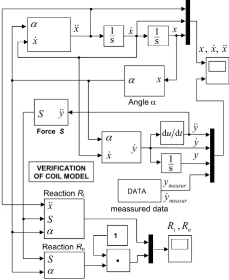
Figure 3. Simulation model scheme g
m3 y
H m3
x 1 S 1 S 2 M 2 2M I 2 I 1 1,I m 1 1x m n R t R B 1 r r1A 2 r 2 S 2 S 1 1M
I M1
H g m1 [ D D
Figure 1. Mechanic scheme of the system
P
cPrel
cP
x cPdrift
D D 1 M Zrel x y cPD
S
S
Figure 2 Kinematical structure
VERIFICATION OF COIL MODEL
DATA meassured data 1 D x x s 1 s 1
x x
D
Angle D
x
D x y
t u d d s 1 y y y measur y measur y x S
D Rt,Rn
S y
Reaction Rt
S D
Reaction Rn
x x x, ,
[image:2.595.95.258.564.740.2]With respect to the complexity of the relation for α(x), which is not a function of ·x, the derivation of the sin α function can be performed numerically in a simulation model.
[image:3.595.68.278.57.220.2]ReSultS
Figure 3 shows the model scheme in the Mat-lab-Simulink program. Figures 4 and 5 show time flows of kinematical values for the coil and weight motion.
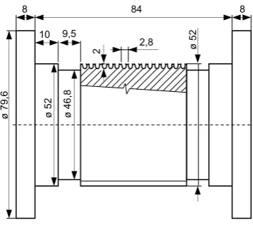
The physical model for the validation of the nu-merical model is shown in Figure 6 and the detail of coil is in Figure 7. The photo of the model is pre-sented in Figure 8.
The direct measurement of the coil position is technically difficult, so an indirect method was chosen which compares the weight position during the validation of the model characteristics. The x
coil position must be converted to the y weight posi-tion in the numerical model using the Eq. (5) with subsequent integration. The weight position relates to the pulley displacement, which is scanned by an incremental sensor.
The determination of the initial conditions value for the numerical model is rather complicated, so the problem of the coil position measurement cannot be avoided. However, the problem can be bypassed so that the coil passage through the optical gate is scanned in the known position of xopt = x(t = 0). The
Figure 6. Physical model arrangement -0,4 -0,2 0,0 0,2 0,4 0,6 0,8 1,0
0 5 10 15 20 25 30 35t(s) 40
x (m)
x (m.s-2)
x (m.s-1)
Figure 4. Coil distance, velocity and acceleration
-0,1 -0,1 0,0 0,1 0,1 0,2 0,2
0 5 10 15 20 25 30 35t(s)40
x (m.s-1) x(m)
[image:3.595.309.515.58.219.2]x (m.s-2)
Figure 5. Weight distance, velocity and acceleration
r2
xopt
Optical gate
for determination of initial conditions. Once shaded the logical input becomes 0
r1B
m1,,I1
+M2
m3
I2
Initial position of the coil
When released the coil is moving towards the pulley
Incremental sensor (2000 imp/rev) Scanning the pulley displacement
(angleM2)
ød
[image:3.595.62.493.257.332.2]H r1A
Figure 5. Weight distance, velocity and acceleration Figure 4. Coil distance, velocity and acceleration
m3g + ·x2 m
3 +I2 d(sinα) r1B – sinα + ξsgn
·
x cos α – m
1g sinε + ξsgn
·
x cosε
r22 dx r1A r1A r1A
·x = (9)
m
3 +
I2 r1B
– sinα) r1B– sinα + ξsgn ·x cos α + m 1 +
I1 r22
r1A r1A r1A r1A2
[image:3.595.117.471.576.734.2]coil velocity ·x(t = 0) can be determined in this posi-tion from the calculaposi-tion resulting from Eq. (5). The required velocity ·y can be determined from the nu-merical derivation of the measured position y. The physical model parameters (weights, moments of inertia, etc.) are set by measuring and weighing, the
8 84 8
10 9,5
ø
79
,6
ø
52
ø
46
,8
ø
52
2,8
[image:4.595.69.247.61.219.2]2
Figure 7. Detail of coil
0,10 0,12 0,14 0,16 0,18
0 5 10 15 20 25 30 35 40
t(s)
y
(m)
calculation measuring
-0,050 -0,025 0,000 0,025 0,050
0 5 10 15 20 25 30 35 40
t(s)
y
(m/s)
. calculation
[image:4.595.67.523.348.728.2]measuring Figure 8. Photo of coil model
Figure 8. Calculated and measured courses of the distance
y
and velocityy
unknown values for the ξ arm rolling resistance and ε plane inclination are determined from sequential optimisation so that the highest conformity of the compared courses is achieved (Figure 9).
ConCluSion
The measuring demonstrated a good conformity in basic parameters, such as the period time, amplitude decrease, stop time etc. Small deviations in the final phase of the motion were most probably caused by fine unevenness of the working plane because the task is very sensitive to its inclination.
The results of simulation shown in the experiment correspond to the exciting of the system by the moment of the motor drive (supplied with square wave voltage). The measured time-dependents of the truck position x, truck velocity v = ·x, amplitude
Figure 10. Comparison of measured and computed kinemat-ical quantities for model of the truck
-0,2 -0,10,0 0,1 0,2 0,3 0,4 0,5
0 2 4 6 8 10 12 14 16 18
x(m)
t(s)
-0,8 -0,6 -0,4 -0,20,0 0,2 0,4 0,6 0,8
0 2 4 6 8 10 12 14 16 t(s)18
v(m.s-1)
-30 -20 -10 0 10 20 30
0 2 4 6 8 10 12 14 16t(s)18
M0)
-3 -2 -1 0 1 2 3
0 2 4 6 8 10 12 14 16t(s)18
Z(rad.s-1)
gear truck
pendulum
motor
trolley x
H M
T
[image:5.595.69.287.260.578.2]M
Figure 9. Model of the truck
solution of the mathematical model (dashed line) are compared in Figure 10. A detailed description of this problem is in Vodřich et al. (2001).
The results prove the correctness of the mathemat-ical description, computer simulation, and adequate accuracy of the applied method identification of the system parameters.
The system described and checked in the article will probably not find direct use in practice. How-ever, the philosophy of mathematical simulation mentioned and the experimental verification of dynamic systems are usable in different engineering spheres, e.g. in the research, proposal, and construc-tion of agricultural machines.
References
Bedford A., Fowler W. (2005): Engineering Mechanics – Statics & Dynamics. 4th Ed. Pearson Education, Upper Saddle River, New Jersey.
Beer F.P., Johnston E.R. (1988): Vector Mechanics for Engineers (Statics, Dynamics). 5th Ed. Mc Graw-Hill Book Company, New York.
Jirků S., Vondřich J. (2002): Analysis of manufacturing systems with asynchronous motors. In: Proc. 12th Int. Conf. Flexible Automation and Intelligent Manufacturing. Oldenbourg Wissenschaftsverlag, München, 26–33. Jirků S., Kočárník P. (2004): Simulace dynamických soustav
s nelineárními odpory a vazbami. In: Proc. IX. Int. Conf. on the Theory of Machines and Mechanisms, Technical University of Liberec, Liberec, 403–408.
Jirků S., Kočárník P. (2005): Simulační model Stirlingova motoru. In: Sborník 46. mezinárodní konference kateder částí a mechanizmů strojů. Technická univerzita, Liberec, 125–128.
Kočárník P., Jirků S. (2006): Simulation of systems with mechanical, hydraulic and temodynamic elements. Jour-nal of Machine Engineering. Efficiency Development of Manufacturing Processes. 6: 104–114.
Vondřich J., Jirků S., Kočárník P. (2001): Identification and Optimization of Parameters of Machine. In: 16th Int. Conf. on Production Research. CTU, Prague, 143.
Received for publication April 4, 2007 Accepted after corrections June 6, 2007
Abstrakt
Kočárník P., Jirků S. (2007): Model kmitajícího systému s cívkou a jeho ověření. Res. Agr. Eng., 53: 182– 187.
Článek je ukázkou řešení dynamické soustavy se složitou kinematickou vazbou a s odporem valení v programu Mat-lab-Simulink. Pro ověření simulace byl zkonstruován fyzikální model s inkrementálním čidlem, které umožňuje snímání a měření kinematických veličin za pohybu soustavy. V příspěvku je uvedeno blokové schéma simulačního
of pendulum ϕ and angular velocity ω = ·ϕ with
modelu a vypočtené průběhy kinematických veličin. Numerické výsledky jsou porovnány s reálným modelem. Měře-ní prokazuje dobrou shodu v základMěře-ních parametrech, jako je doba periody, pokles amplitudy, doba zastaveMěře-ní apod. Malé odchylky v konečné fázi pohybu mohou být způsobeny drobnými nerovnostmi základové desky při experimen-tu. V závěru jsou stručně popsány i výsledky ověření simulace soustavy vozíku s kyvadlem.
Klíčová slova: dynamické soustavy; matematický model; simulace; ověření
Corresponding author:
Doc. Ing. Slavomír Jirků, CSc., České vysoké učení technické v Praze, Fakulta elektrotechnická, katedra mechaniky a materiálů, Technická 2, 166 27 Praha 6, Česká republika