Application of 3D cameras in agriculture when evaluating the quality of soil tillage

Application of 3D cameras in agriculture when evaluating

the quality of soil tillage

M. Kříž, M. Linda, J. Svatoš, M. Hromasová

Department of Electrical Engineering and Automation, Faculty of Engineering,

Czech University of Life Sciences Prague, Prague, Czech Republic

Abstract

Kříž M., Linda M., Svatoš J., Hromasová M. (2016): Application of 3D cameras in agriculture when evaluating

the quality of soil tillage. Res. Agr. Eng., 62: 39–49.

The paper deals with the evaluation of data collected by scanning the agricultural surface with a 3D Photonic Mixer Device (PMD) camera with IFM company electronics and a resolution of 64 × 50 pixels in different scanning modes. After short introduction various methods of measuring of soil surface characteristics are presented. These methods are laser, photogrammetric and radar measurement followed by experimental measurement by kinect system and O3D201 3D camera using the Photonic Mixer Device (PMD) technology. For 3D calibration measurements of the camera a quartered pyramid model was used. Measurement results before and after the field testing area soil tillage are presented.

Keywords: PMD sensor; picture; model; soil roughness; measurement

Electronic devices are used in modern precision agriculture techniques. The emphasis is to improve the soil condition of a field during soil tillage based on existing yield and application maps. In order to improve and maximise the effort in soil condition-ing of a field a simple and cost effective method to scan and analyse the existing soil condition is required. Compared to other systems (on board) camera systems have considerable advantages for this kind of use. They provide a contactless applica-tion and the possibilities of complex evaluaapplica-tion of the scanned area. They have, however, few signifi-cant disadvantages, for example: the sensitivity and the readability in various lighting conditions and significant ambient influences.

At present the available ways of setting up the re-quired parameters during the operation of soil till-age equipment, are limited. The influence of

differ-ent soil conditions causes that the equipmdiffer-ent does not perform the desired function correctly. The op-erator can however, make changes in the settings, but this is mostly a temporary and subjective so-lution. As a result, it can lead to uneven seedbed preparation, and a subsequent lack of crop germi-nation. Electronic systems can be used to perform a quality assessment of the soil tillage, either by con-tact or concon-tactless bearings approaches.

The situation described above gave rise to a re-quirement to develop a system that would enable the collection of data about the roughness surface of a field. On the basis of the measured data, the sys-tem would inform operators, whether it is necessary to optimise the settings of the equipment. The next step would be to link the system with the active parts of the working equipment, and thus to achieve auto-matic adjustment according to the current soil and

1 27

53 79

105 131

157

0 20 40 60 80 100 120 140 160

1

16

31

46

61

76

91

106

121

136

151

166

181

196

211

226

241

256

271

286

ambient conditions. At present the measurement of surface roughness is solved by a single-purpose portable instruments which are placed on the field before the passage of agricultural soil tillage equip-ment such as plough or harrows and after tillage. The role of the soil measurement coarseness and the related actuators control of agricultural machinery working parts have not been addressed in this paper.

At present for contactless measurement of the roughness and homogeneous character of the soil, laser, photo-gravimetrical and Synthetic Aperture Radar (SAR) systems are used.

Laser systems can be used to assess the impact

of the soil surface structure on the movement of the substrate due to water and wind erosion (Hau-brock et. al. 2009). Laser scanning was also previ-Fig. 1. An example of the Kinect application (a) depth image and (b) camera image

X, Y, Z – accelerometer data (Kinect sensors)

(a) (b)

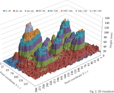
Fig. 2. 3D visualization of the Kinect data Pixe

l coor_dina

te Y (–) Pixel co

ordinate X (–)

H eight (mm)

ously used for the detection of height differences (Huang et al. 1990). High resolution in the hori-zontal and vertical direction is an undisputed ad-vantage of laser scanners and therefore these scan-ners, in comparison with other photogrammetric methods, are suitable for measuring fine structured regions (Flanagan et. al. 1995). In order to obtain a three-dimensional model of the scanned area by means a laser scanner, it is necessary to scan the surface of the land at 90° from the vertical gradient of the axis below the azimuth between 45° and 65°. After data processing, a three-dimensional model is created and then the roughness indexes are as-signed.

Photogrammetric measurement. In the area

of photogrammetric measurement (Jester, Klik 2005) two identical cameras placed perpendicu-larly to the measured area at a height of 1,200 mm are used. Photos are converted to black and white negatives by means of a photogrammetric scan-ner. To obtain three-dimensional data, negatives are further converted into digital points by means of a photogrammetric station using the Intergraph ISPM software. A three-dimensional model is then generated from these points. With this method, the time required for the measurement and evaluation can take up to 125 minutes.

Radar measurement. Radar measurements of

the soil surface are used to estimate soil moisture and granularity. Such mapping is carried out on a larger scale and the acquired data does not always have to correspond to the reality, because the radar signal is sensitive to the reflectance from the soil surface or other debris fragments. Another factor affecting the measurement is the fact that the radar signal penetrates the surface of the soil and partly, by the granularity of the surface measurements, may be distorted. Several models are used for the processing of data from radar measurements, most frequently an integral equation model (IEM) (Rah-man et. al. 2008).

Experimental measurement.An alternative

Ki-nect sensor can be possibly used for measuring the roughness character of soil. This sensor takes the role of a computer games control by means of the player´s body motion. The features of this sensor equal and, in some applications, exceed the camera systems. A disadvantage of Kinect is in its indoor use and in its higher demands for computing pro-cessing of collected data. Its disadvantage for agri-cultural use is the requirement for object

resolu-tion of at least 1 cm. Fig. 1 presents a sample system in the image of the testing area of the field. The sen-sor enables viewing the shot from the web camera Kinect together with data (of a distance vector) at a resolution of 640 × 480 pixels. The system also in-cludes microphones, 3-axes accelerometer, sensor directing in the horizontal axis, and the option of installing the “Skeleton stream” tool. Fig. 2 shows the processing and thresholding of the measured data. Presented data are shown in 3D graph. In Fig. 2 you can see the min. resolution of an object in the picture and the overall resolution of the pic-ture that is real.

The O3D201 camera system, which uses the PMD technology, has several sensors arranged in a matrix on a ½" chip. This arrangement enables to measure the whole scene in one moment. The light-ing of the scanned scene is ensured by the internal source of modulated infrared light. Reflected light rays are then captured through the optical system on the PMD matrix. The distance of the scene is then computed from the correlation between the emitted and reflected rays. This obtains a distance value for each pixel (Mlatecová et al. 2011).

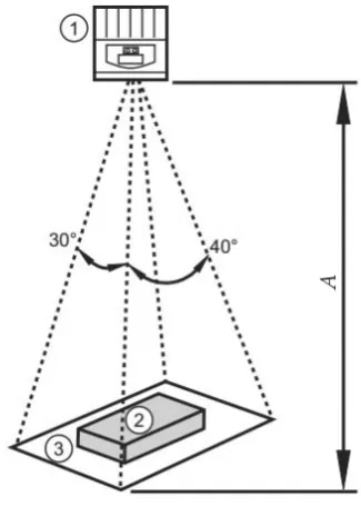
The 3D camera captures an image scene in both intensity and distance. For correct analysis, it is necessary to perform a calibration and detect the sensitivity and resolution of the camera due to the

Fig. 3. Schematic sketch of (1) camera, (2) measured object and (3) visual field arrangement during measurement, where A is the distance of the camera from the base of the measured object (ifm electronic 2013)

number of camera pixels being 64 × 50. Both the measurement and calibration is shown in Fig. 3, where the situation during the measurement and calibration is displayed.

MATERIAL AND METHODS

Measurements for the calibration of output data from the PMD camera (O3D223; ifm electronic gmbh, Essen, Germany) took place at three height levels: 500 mm, 1,000 mm and 1,500 mm. The cali-bration and entry of collected data were performed for each level. The calibration covered two modes of operation the intensity and the distance to the object. During the measurement, the exposure set-ting has been changed. The camera was equipped with an internal source of lighting, which is suffi-cient for our application; external lighting systems should be considered for add-on measurement ap-plications.

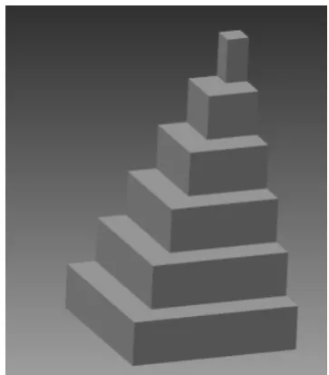
For analysis of the camera sensitivity and resolu-tion, a quartered pyramid model was created (Fig. 4). This features a defined rise of individual floors. Dimensions of the base of the model were 115  × 115  mm, height 180 mm, rising 30 mm and each floor was decreased by 20 mm in length and width. The rise of the model floors corresponds to the min. resolution required for possible measurement of soil roughness. The camera output data are presented in supplied software as the surface presentation of the

distance vector, distinguished by a colour or by a 3D chart of a shot of the visual field of the camera.

Catalogue parameters of the 3D camera for speci-fied measurement heights are listed in Tables 1 and 2. The specified measurement heights are selected for the possible application of the system in agricul-ture soil studies, such as determining the quality of processed soil following the passage of a soil tillage machine.

The software supplied with the camera is fully ca-pable for the calibration requirements. For meas-urement, this system lacks the sequential saving of images to create a 3D model. An application that Table 1. Image size parameters for experiments, visual field (ifm electronic 2013)

Measuring range (mm) Length (mm) Width (mm) Minimum object size (mm)

500 420 290 13 × 13

1,000 840 580 26 × 26

1,500 1,260 870 39 × 39

Table 2. Image size parameters for experiments, recommended exposure time (ifm electronic 2013)

Measuring range (mm) White 90% (ms) Grey 18% (ms) Black 6% (ms)

Recommended exposure

500 8 9 14

1,000 9 17 27

1,500 11 27 27

Repeatability of the distance depth measurement

500 ± 5 ± 8 ± 16

1,000 ± 5 ± 8 ± 16

1,500 ± 5 ± 9 ± 17

enables to perform basic camera settings and se-quential reading of data was therefore programmed using the Visual Basic 2010.net programme (Mi-crosoft, Redmond, USA).

Communication for settings was carried out on port 8080, IP address 192.168.0.69. Shot data were read from camera port 50002. The camera was set up by the XML-RPC protocol, which was based on the principle of remote procedure call. Requirement specification consisted of a header and a body. The data file from the camera had a similar structure. Precise specification and the format of the request were included in the documentation of the protocol and in the documentation for the 3D camera.

Calibration blocks (a), (b), (c) are presented in Fig. 5. Calibration blocks were used for the calibra-tion of the camera in the mode „intensity“. This en-ables un-thresholding of the output data according to the settings mode.

RESULTS AND DISCUSSION

The movement of the agricultural machinery was not taken into account within the experiment as the experiment is concerned with the application of static scanning. Real pictures of calibration pat-terns are shown in Fig. 6a. These shots represent Fig. 5. Calibration intensity blocks (a) Stasiuk (2013); (b) Šulc (2013); (c) ČVUT (2013)

(a) (b) (c)

Fig. 6. Recording for (a) dimensions of 75 mm × 4.5 mm at the height of 500 mm, exposure of 15.2 ms and (b) dimen-sions of 75 mm × 4.5 mm at the height of 1,000 mm, exposure of 17.3 ms (left image – perspective model, right image – mesh network); image on the left presents the output of intensity, the one in the right presents the shot distance vector and third shows the image converted into 3D view

(a)

(b)

1%

0% 50%

100% 95%

20% 40% 62% 80%

96% 97% 98% 99%

2% 3% 4% 5%

0 1 2

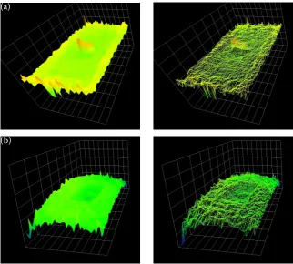
Fig. 8. Testing area of the field (a) before and (b) after the tillage (left image – top view, right image – skewed view) Fig. 7. Calibration picture of the model at the height of (a) 500 mm and of (b) 1,000 mm (left image – perspective model, right image – mesh network)

(a)

(b)

(a)

Fig. 9. 3D camera control inter-face and colour range of distances (resolution of 64 × 50 pixels)

Fig. 10. Testing area of the field before tillage; measured at the height of (a) 500 mm, (b) 1,000 mm and (c) 1,500 mm (left image – perspective model, right image – mesh network)

(a)

(b)

Fig. 11. 3D visualisation of the testing area of the field (a) before tillage and (b) after tillage at the height of 500 mm

Table 3. Exposure parameters for individual measurement heights

Height (mm) 500 1,000 1,500 Exposure 1 (ms) 15.70 17.30 22.40 Exposure 2 (ms) 16.50 18.20 19.20

Exposure 1 – exposure light in measuring area before tillage; Exposure 2 – exposure light in measuring area after tillage

1 4 7

10 13 16 19 22

25 28 31 34 _{37 40 43 46}

49 0 20 40 60 80 100 120 140 160 180 1 5 9 13 17 21 25 29 33 37 41 45 49 53 57 61

0–20 20–40 40–60 60–80 80–100 100–120 120–140 140–160 160–180

1 4 7

10 13 16 19 _{22 25 28 31}

34 37 40 43 _{46 49}

0 20 40 60 80 100 120 140 160 180 1 5 9 13 17 21 25 29 33 37 41 45 49 53 57 61

0-20 20-40 40-60 60-80 80-100 100-120 120-140 140-160 160-180

camera capacities to capture the colour intensity of objects.

Minimum resolution is simulated on an object with dimensions of 75 mm × 4.5 mm and 75 mm × 8 mm. Fig. 6b shows the output for the dimensions of 75 mm × 4.5 mm at a height of 500 mm. This should be compared with Fig. 7a where there is a noticeable difference in the loss of information about the object size. In Fig. 7a the dimensions are 75 mm × 4.5 mm at a height of 1,000 mm. The measurement was carried out identically for the height of 500 mm, 1,000 mm and 1,500 mm. In or-der to increase the contrast the object had to be placed on a white pad of 210 mm × 297 mm. For

the camera height of 1,500 mm the object cannot be detected.

Height and surface resolution is an important parameter for the application of the camera dur-ing soil tillage measurements. The followdur-ing images (a)

(b)

Pixel coordina_{te Y (–)}

Pixel coordina_{te Y (–)}

Pixel coordina te X (–)

Pixel coordina te X (–)

Heig ht (mm)

show the height resolution for defined measurement heights. It specifies the minimum object size that can be captured by the evaluation system. Camera images of the created quarter pyramid model (Fig. 4) are shown in Fig. 7. The bevel of edges in sharp cross-ing of the wall can be seen of these pictures. For the camera height of 1,500 mm quartered calibration pyramid was spatial deformed as seen in Fig 7b.

Testing area of the field before and after tillage

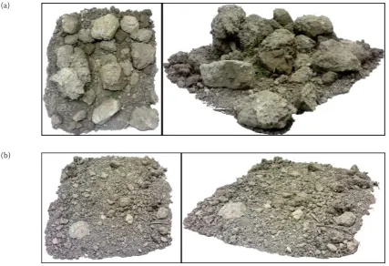
Fig. 8 shows the results of the application soil measurement. The scanned testing area of the field

before tillage has the dimensions of 500 × 600 mm, the highest point measures 167 mm and the point in the middle of the field measures 125 mm. This testing area of the field after tillage has the same di-mensions and the highest point of the scanned area measures 50 mm. The parameters of the scanned area before and after tillage are presented in Table 3.

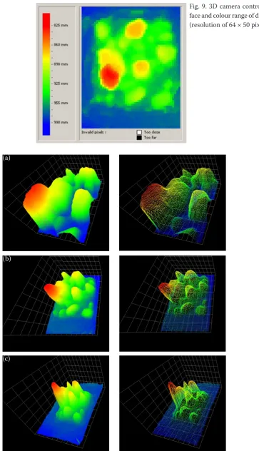
During the measurement, the 3D camera was placed on a tripod above the measured area. The output of the measurement included shots of the intensity, a 3D model with edge rendering and 3D network model. The images were exported from the 3D camera control interface. Grayscale colour-ing of the pictures corresponds to the distance from the scanner to the measured area. The application Fig. 12. Testing area of the field after tillage; measured at the height of (a) 500 mm, (b) 1,000 mm and (c) 1,500 mm (left image – perspective model, right image – mesh network)

(a)

(b)

for the recording of data from the IFM camera is shown in Fig 9.

Fig. 10a presents the non-processed soil meas-urement from the height of 500 mm. Compared to Fig. 10b and Fig. 10c there is a noticeable impact of the measurement height on the distortion of meas-ured data.

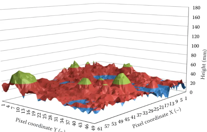
Fig. 11a and Fig. 11b shows data processing; the x and y axes show the picture resolution of the cam-era sensor and axis height (mm) shows the verti-cal verti-calibration of the measured surface height. This represents the basis for the application parts of the machine during the soil tillage. Fig. 11a shows data before tillage and Fig. 11b shows data after tillage.

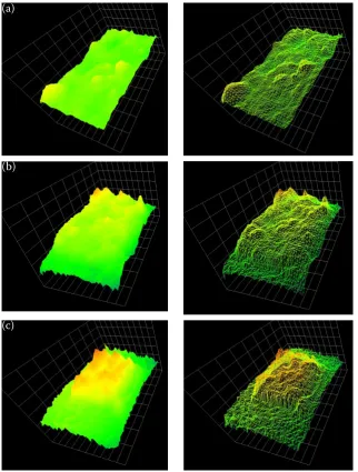
In order to represent the soil sample after tillage the sample was crushed and area re-scanned. There is an obvious difference in the images of the soil condition (Fig. 12) which were taken from the pre-defined heights. This figure should be compared with Fig 10.

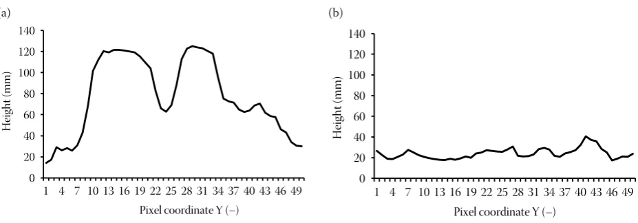
A longitudinal section profile in the middle of the testing area of the field was created to compare

both scanned areas. The results of the proxy soil tillage can be seen from the curves (Fig. 13). To es-tablish a soil tillage quality indicator of the testing area of the field before and after tillage was made using the percentage height differences. The pro-cessing ratio RP_n of the testing area was computed by Eq. (1).

RPn= An

−Bn

(

)

kmin−kmax ⎛

⎝⎜

⎞

⎠⎟×100 (%) (1) where:

k_min – min(A_n – B_n) (mm) k_max – max(A_n – B_n) (mm)

A_n – height of the soil in nth_{coordinate of y axis of the}

testing area before tillage (mm)

B_n – height of the soil in nth_{coordinate of y axis of the}

testing area after tillage (mm)

The resulting ratio of processing is shown in Fig 14.

CONCLUSION

The contribution of this paper was to assess the quality of information measured by an industrial 3D camera. From the measured data soil conditions before and after treatment can be determined. The system is easy to use and does not require specialist and additional expensive software. The calibration was carried out on the model and on the calibra-tion blocks. Subsequently, the measurements of static soil surface shot were carried out. The possi-bility of programming a 3D camera by the XML-PC protocol was also presented. The use of 3D cameras might be useful in determining the state of soil till-age and in a more objective setting that of machine Fig. 13. Sections profile of the testing area of the field (a) before and (b) after tillage from the height of 500 mm

1 4 7 10 13 16 19 22 25 28 31 34 37 40 43 46 49

H

ei

gh

t (

mm)

Pixel coordinate Y (–)

0 20 40 60 80 100 120 140

1 4 7 10 13 16 19 22 25 28 31 34 37 40 43 46 49

H

ei

gh

t (

mm)

Pixel coordinate Y (–)

1 4 7 10 13 16 19 22 25 28 31 34 37 40 43 46 49

H

ei

gh

t (

mm)

Pixel coordinate Y (–)

0 20 40 60 80 100 120 140

1 4 7 10 13 16 19 22 25 28 31 34 37 40 43 46 49

H

ei

gh

t (

mm)

Pixel coordinate Y (–)

(a) (b)

Fig. 14. Processing ratio of the testing area

0 10 20 30 40 50 60 70 80 90 100

1 4 7 10 13 16 19 22 25 28 31 34 37 40 43 46 49

Ra tio of p roc es sing (% )

Pixel coordinate Y (–)

Vol. 62, 2016 (2): 39–49 Res. Agr. Eng.

surface roughness from in-situ laser scanning. Catena, 79: 128–139.

Huang C.H., Bradford J.M. (1990): Portable laser scanner for measuring soil surface roughness. Soil Science Society of America Journal, 54: 1402–1406.

ifm electronic (2013): Datasheet catalog. Available at http:// www.ifm.com

Jester W., Klik A. (2005): Soil surface roughness measure-ment—methods, applicability, and surface representation. Catena, 64: 174–192.

Mlatecová H., Žalud L. (2011): Optical proximity sensor with time-of-flight measuring principle. In: Sborník prací konference a soutěže Student EEICT 2011. Available at http://www.feec.vutbr.cz/EEICT

Rahman M.M., Moran M.S., Thoma D.P., Bryant R., Holifield Collins C.D., Jackson T., Orr B.J., Tischler M. (2008): Map-ping surface roughness and soil moisture using multi-angle radar imagery without ancillary data. Remote Sensing of Environment, 112: 391–402.

Stasiuk G. (2013): Calibration picture. Available at http:// uofgts.com

Šulc V. (2013): Calibration picture. Available at http://www. viktorio.net

Received for publication March 17, 2014 Accepted after corrections June 7, 2014 parameters for soil tillage. These improvements

will lead to better soil tillage and help to achieve higher crop yields. Higher purchase of the camera and complicated operation may be a possible draw-back. Further research is needed which will involve full field trials and then mounting on agricultural machinery to determine the impact of movement and vibration on the camera images. In the future the other possibilities of detecting the soil using proprietary sensors or different methods of surface characterization will be done. The resulting sys-tems could find use even under dynamic measure-ment and the implemeasure-mentation of specific solutions.

References

ČVUT (2013): Calibration picture. Available at http://cmp. felk.cvut.cz/cmp/courses/Y33DIF/2009-2010LS

Flanagan D.C., Huang C., Norton L.D., Parker S.C. (1995): Laser scanner for erosion plot measurements. Transactions of the American Society of Agricultural and Biological Engineers, 38: 703–710.

Haubrock S.N., Kuhnert M., Chabrillat S., Guntner A., Kaufmann H. (2009): Spatiotemporal variations of soil

Corresponding author: