Economic aspects of rural areas sustainable development

INTRODUCTION

In the last ten years of transformation of the econo-my, Czech agriculture has been experiencing a number of positive changes in building up of background for efficient market agrarian sector. However, the present model of economy was formed in a different historical context, i.e. in different economic, social and civiliza-tion condiciviliza-tions – in times when there seemed to be enough resources and space for unlimited growth, for unlimited consumption of the resources and unlim-ited production of waste. According to the present knowledge, however, the mankind is already facing and exceeding the limits of the Planet bearing capacity which makes this economic system unsustainable and replacing it with an alternative system that respects sustainable development principles is an important

precondition for preserving diversity of life forms and favorable environment for life of the humans. More and more economists realize the limitation and finiteness of the resources that economy uses for growth of production, cash-flows and consumption. According to some economists, economy is interpreted as non-growing system and its quantitative growth cannot continue forever. It does not mean going back to simple civilization habits but efficient management of natural resources, taking from the nature only as much as it is able to regenerate, using eco-effective technologies, recycling wastes to the maximum extent and reducing useless consumption.

The state of natural resources is significantly influ-enced by agricultural activities which are not equally spread over the area of state, but differently in indi-vidual regions. Nevertheless, agricultural production is

Economic aspects of rural areas sustainable development

Ekonomické aspekty udržitelného rozvoje rurálních oblastí

J. TVRDOŇ

Czech University of Agriculture, Prague, Czech Republic

Abstract: The articles deals with problems of different development of rural areas and their factors. In usual analysis of rural

development, the position of agriculture is interpreted in broad range of opinions from the neglectable role to its non-substituta-bility in rural economics. The article follows strong sides of these concepts at simultaneous reduction of their weaknesses and is focused on problems of investigation of the mutual influence of endogenous as well as exogenous industries on rural regions. Applied approach leads to setting up model of economic base and deriving of multiplicators of rural development. It is obvious from the analysis that nonagricultural subsidy programs supporting development of the others industries in region have indirect influence upon its agriculture too. In different regions, this influence varies due to the factors investigated in the paper.

Key words: regional economics, economic base models, multiplicators of economic development, employment, inter industries

relationships

Abstrakt: Článek se zabývá problémy různého rozvoje venkovských oblastí a jejich faktory. V obvyklé analýze je pozice venkovského rozvoje zemědělství v široké paletě názorů od zanedbatelné role až k její nezastupitelnosti ve venkovské ekonomice. V práci jsou uvedeny silné stránky těchto pojetí při současné redukci jejich slabých stránek a je zaměřená na problémy výzkumu vzájemného vlivu endogenních a exogenních odvětví na venkovské regiony. Aplikovaný přístup vede k vytvoření modelu ekonomické báze a odvození multiplikátorů venkovského rozvoje. Z analýzy je zřejmé, že nezemědělské dotační programy podporující rozvoj jiných odvětví v regionu mají nepřímý vliv také na zemědělství. V různých regionech je tento vliv různý v závislosti na sledovaných faktorech.

a part of industries mix almost in every region. From this viewpoint, agriculture industry is in interactions with the other industries in each region. The types of those interactions are multidimensional, but for the limited scope of this article only two, but basic relationships will be analyzed.

AIMS AND METHODOLOGY

The main goal of the paper is to investigate mutual interdependency between agriculture and other in-dustries in different regions in the Czech Republic on the base theory of regional development (Tvrdoň 1994).

The working hypothesis follows these assump-tions:

– Rural areas are part of all administrative regions of the Czech Republic

– Economic and environmental performance of agri-culture is interlinked with the total region economic and environmental performance

– For explanation of this relationship, model of eco-nomic base can be used

– Level of employment in regions depends on the national rate of employment and structure of in-dustries in that region.

Joint background for these assumptions is explained by (Isard 1990) and others (Stillwell 1992) who suppose that growth in one regional industry is the function of growth of all industries in that region. If the rest of economy operates well, one industry in a role of input from those industries is predetermined to operate successfully too and vice versa. Due to the lack of data of rural regions, data published by the Czech Statistical Office for 13 administrative regions were used (Statistická ročenka 2003).

Applied methods were predetermined by investi-gated the problems which were according to the above mentioned structure, but in all parts it was dealt, even though in a different rate, with qualitative analysis, quantitative analysis, synthesis, comparison, method of analogical conclusions, norm method, interview-ing, elaboration of documents and others.

RESULTS OF ANALYSIS

Specification of Economic Base Model (EBM)

In the EBM, all industries of given region are devided into two groups on the hypothesis of high depend-ency of regional performance measured by income and employment upon the basic sector which delivers

its product and services to buyers of others regions. Non-basic sector provides products and services first of all inside of the given region. To this definition, agricultural industry fits the most.

To derive the multiplicator of economic base, total income of region can be devided into two parts:

T = S + B (1)

T = total income of region S = Income of non basic sector B = Income of basic sector

The amount of income created by non-basic sec-tor depends on income created by region as a total. The greater the income, the greater the demand for products and services provided in framework of given region.

S = sT (2)

From (1) and (2) it can be derived

(3)

where 1/(1 – s) is multiplicator of economic base. If for example T/B = 1.5, income increase in basic sec-tor by 100 CZK will stimulate total income increase of region by 150 CZK.

Multiplicator of employment can by derived simi-larly by substitution data of employment for data of income. Where considering also influence of other factor on the total region income, the previous model can be adjusted:

S = s₀ + s₁T (4)

From (1) and (4), it can be derived:

(5)

For deriving both multiplicators, regression models can be applied.

Specification of regional structure of employment analysis (RSEA)

Under the hypothesis that economic situation of region significantly influences its agriculture, the following analysis can specify the impact of industry structure upon employment development.

Application of the RSEA follows these relation-ships

B s s s

T �

� � � �

1 1 0

1 1 1

. 1

1 _B

s

T �

1. Regional employment growth (g_r)

(6)

r_i = regional employment in industry “i”

= number of employed in all industries in given region

t, o = last and reference year of analyzed time period

2. National employment growth (g_n)

(7)

Specification of variables and indices is the same as in (6) only instead of regional level, variables are from the macro level.

3. Regional employment growth in nationwide em-ployment growth rate

(8)

Variable (g_rn) expresses growth of regional employ-ment if each industry had the same growth rate as that on the nationwide scale.

From these relationships, it follows:

Regional employment growth = Growth induced by other factors + Growth following industry mix + Nationwide growth rate impact

g_r = (g_r – g_rn) + (g_rn – g_n) + g_n (9)

The higher the component g_n the higher the growth of employment in regions.

Expression (g_rn – g_n) manifests structural compo-nent impact of industry structure in given region on employment. If industry structure supports employ-ment, the expression is positive (g_rn > g_n). The op-posite means that industry structure is not suitable for employment development.

Expression (g_r – g_rn) manifests that part of growth which was induced by other factors not included in the model. Positive values mean that employment in region is faster than it would be if employment growth in every industry were the same as at the national level.

Deriving and analysis of the model’s parameters Impact analysis of regional economic

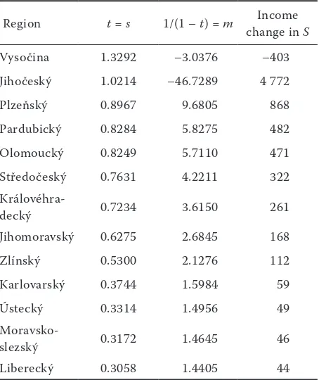
development on income level in agriculture For the analysis, models (2) and (4) were specified with parameters enabling to rank regions according to the influence of the total region income level upon the income level in agriculture considered as non-basic sector (Tvrdoň 2003). Table 1 presents the output.

Results of calculations are ranked up according to size of “t” at row 1. Figures at row 2 are multiplicators “m” according to equation 3 explaining total income change in the given region induced by unit change of income in basic sector. From it, row 3 is calculated and the results express what will induce income change by 100 CZK of basic enterprises in agriculture. In the region Vysočina for example, income will decrease by 403 CZK and it will increase income in agriculture of the Liberec region by 44 CZK. If regional economy improves, income level of agriculture industry goes up by t times – specially in the Vysočina and Jihočeský regions. The other results are documented by follow-ing Figure 1.

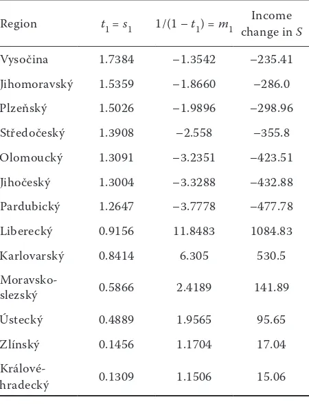
More reliable model is the relationship (4) which admits also other influences expressed by “t₀” values for individual regions. For the restricted size of the article, “t₀” values are not presented and only “t₁” parameters are analyzed according to Table 2.

�

r

100 0

0

� � �

�

�

�

i i i i i

t i r

r r r g

100 0

0

� � �

�

�

�

i i i i i

t i n

n n n g

100 /

0 0 0 0

� � � � � �

� � �

�

�

�

i i

i i i i

t i i rn

r r n n r g

Table 1. Structural parameter “t” of equation S = tT, multi-plicators and income changes

Region t = s 1/(1 – t) = m _{change in S}Income

Vysočina 1.3292 –3.0376 –403

Jihočeský 1.0214 –46.7289 4 772

Plzeňský 0.8967 9.6805 868

Pardubický 0.8284 5.8275 482

Olomoucký 0.8249 5.7110 471

Středočeský 0.7631 4.2211 322

Královéhra-

decký 0.7234 3.6150 261

Jihomoravský 0.6275 2.6845 168

Zlínský 0.5300 2.1276 112

Karlovarský 0.3744 1.5984 59

Ústecký 0.3314 1.4956 49

Moravsko-

slezský 0.3172 1.4645 46

The analysis of the results is analogical to model (2) but for all equations, R2 _{indicators is created to}

the level 0.75–0.95. Income increase by 100 CZK in basic industries has symmetrical impact upon income level in agriculture – aprox. half of regions manifest decrease of agricultural income whereas the second half shows income increase. For example in the region Vysočina, there is decrease of 235.4 CZK in agricul-tural income, whereas the region Královéhradecký and Zlínský manifest an increase of agricultural income by 15.06 CZK, respective Zlínský, 17.04 CZK.

Parameters “t₁” for all regions are presented in Fig-ure 2.

Income level m₀ = t₀/(1 – t₁) which remains on that level even though income level of basic sector will go up fall down. For explanation of changes in the region ranking, it would be necessary to analyze more comprehensive database than those which are available and a wider scope of the paper.

Impact analysis of regional industry structure upon employment development

Region economic performance can be analyzed ac-cording to many indicators but at least two of them

Table 2. Structural parameter “t₁” of equations S = t₀ + t₁T,

multiplicators, income changes

Region t₁ = s₁ 1/(1 – t₁) = m_{1 change in S}Income

Vysočina 1.7384 –1.3542 –235.41

Jihomoravský 1.5359 –1.8660 –286.0

Plzeňský 1.5026 –1.9896 –298.96

Středočeský 1.3908 –2.558 –355.8 Olomoucký 1.3091 –3.2351 –423.51 Jihočeský 1.3004 –3.3288 –432.88 Pardubický 1.2647 –3.7778 –477.78 Liberecký 0.9156 11.8483 1084.83

Karlovarský 0.8414 6.305 530.5

Moravsko-

slezský 0.5866 2.4189 141.89

Ústecký 0.4889 1.9565 95.65

Zlínský 0.1456 1.1704 17.04

Králové-

hradecký 0.1309 1.1506 15.06

Figure 2. Parameter t₁ of equation S = t₀ + t₁T

(asix x – gt, asix y – region) 0.0 0.2 0.4 0.6 0.8 1.0 1.2 1.4 V ys o � in a Jiho � es ký Plz e � sk ý K ra je - 20 02 Pa rd ub ic ký O lo m ou ck ý St � ed o � es ký K rá lo vé hr ad ec ký Jihomoravský Zl ín sk ý Karlovarský Ú st ec ký Moravskoslezský Li be re ck ý

Figure 1. Parameter t of equations S = tT (asix x – t, asix y – region)

play a non-substitutable role. One of them – income level – is investigated in previous chapter, second one – employment development during time period 1995–2002 and its determinants – are analyzed in the following part of the paper.

For that aim, indicators (6), (7), (8) were calculated and used for decomposition of employment growth according to model (9).

Specification of employment growth in regions

According to relation (6), indicator g_r for time period 1995–2002 was calculated and when ranked from the viewpoint of its size following results are presented.

From the Table 3, it is obvious that the number of employed people fell down in all regions but with large differences. In the Středočeský region for example,

employment decrease is 6.24% whereas in the Ústecký region it was 26.35%. Growth rates for all regions are presented in Figure 3.

Specification of potential employment growth in regions

According to relation (8) indicator g_rn in the given time period was calculated and when ranked from the viewpoint of its size following results are pre-sented.

The Table 4 illustrates significant differences in the potential region employment growth. In the region Karlovarský employment growth could be 27.55%, whereas in the Moravskoslezský only 5.65%.

Potential growth rates for all regions can be clearly seen in Figure 4.

Table 3. Regional growth rate g_r

Region g_r

Středočeský –6.2419

Jihomoravský –7.8611

Liberecký –11.9573

Zlínský –12.4435

Vysočina –12.8469

Královéhradecký –13.6574

Plzeňský –13.8605

Jihočeský –16.0283

Pardubický –18.6980

Moravskoslezský –21.2663

Karlovarský –22.7047

Olomoucký –22.9413

Ústecký –26.3589

-30 -25 -20 -15 -10 -5

0 St

�

ed

o

�

es

ký

Jihomoravský Libe

re

ck

ý

Zl

ín

sk

ý

V

ys

o

�

in

a

K

rá

lo

vé

hr

ad

ec

ký

Plz

e

�

sk

ý

Jiho

�

es

ký

Pa

rd

ub

ic

ký

Moravskoslezský Karlovarský Olo

m

ou

ck

ý

Ú

st

ec

ký

Figure 3. Region growth rates (asix x – gt, asix y – region)

Table 4. Potential employment growth

Region g_rn

Karlovarský 27.5500

Liberecký 19.9413

Vysočina 15.8528

Pardubický 15.7295

Královéhradecký 14.7680

Zlínský 14.3882

Plzeňský 14.3064

Olomoucký 12.9545

Jihočeský 12.9496

Ústecký 9.5637

Středočeský 8.3311

Jihomoravský 6.9369

Specification of national economy employment growth

According to relationship (7), indicator g_n was cal-culated in the given time period and its value is equal to –1.69%

When indicators (6), (7), and (8) were specified, determinants of employment growth according to relationship (9) can be analyzed. For that purpose, three components of growth rate were calculated and all of them are presented in the Table 5.

From the Table 5, it is obvious that industry restruc-turing in all regions has taken place successfully and, if

0 5 10 15 20 25 30

Karlovarský Li

be

re

ck

ý

V

ys

o

�

in

a

Pa

rd

ub

ic

ký

K

rá

lo

vé

hr

ad

ec

ký

Zl

ín

sk

ý

Plz

e

�

sk

ý

O

lo

m

ou

ck

ý

Jiho

�

es

ký

Ú

st

ec

ký

St

�

ed

o

�

es

ký

Jihomoravský

Moravskoslezský

Figure 4. Potential growth rates (asix x – grn, asix y – region)

Table 5. Decomposition of regional growth rates

Region

Regional employment

growth Growth induced by other factors + Growth following industry mix + Nationwide growth rate ímpact

g_r (g_r – g_rn) + (g_rn – g_n) + g_n

g_r = A + B + C

Středočeský –6.2419 –14.5730 10.0180 –1.6869

Pardubický –18.6980 –34.4276 17.4164 –1.6869

Liberecký –11.9573 –31.8986 21.6281 –1.6869

Vysočina –12.8469 –28.6996 17.5396 –1.6869

Jihomoravský –7.8611 –14.7980 8.6238 –1.6869

Ústecký –26.3589 –35.9225 11.2506 –1.6869

Plzeňský –13.8605 –28.1669 15.9933 –1.6869

Zlínský –12.4435 –26.8317 16.0751 –1.6869

Jihočeský –16.0283 –28.9780 14.6365 –1.6869

Karlovarský –22.7047 –50.2547 29.2369 –1.6869

Moravskoslezský –21.2663 –26.9171 7.3378 –1.6869

Královéhradecký –13.6574 –28.4254 16.4549 –1.6869

Olomoucký –22.9413 –35.8958 14.6414 –1.6869

no other negative factors comprehensively quantified in column A would operate, in all regions the rate of employment could be positive – see column B – and relatively at a very high level.

The weakest impact of the other factors is in the Stře- dočeský region (–14.57 %) whereas in the Karlovarský region is more than three times higher (–58.25 %).

Table 6. Growths of employment induced by other factor

Region g _r– g_rn Region g_r – g_rn

Středočeský –14.5730 Jihočeský –28.9780

Jihomoravský –14.7980 Liberecký –31.8986

Zlínský –26.8317 Pardubický –34.4276

Moravskoslezský –26.9171 Olomoucký –35.8958

Plzeňský –28.1669 Ústecký –35.9225

Královéhradecký –28.4254 Karlovarský –50.2547

Vysočina –28.6996

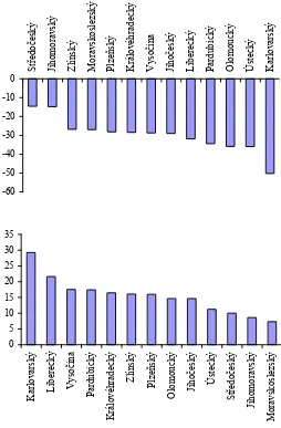
On the other hand in the Karlovarský region, there is relatively very suitable industry composition, but this potential is severely devaluated by other factors. The lowest potential growth due to industry structure is in the Moravskoslezský region. The following table brings results of calculation for all regions.

The data of the table bring more information in the graph form which follows.

In similar sequence of regions, it can be expected that agriculture growth in regions will follow. If growth

-60 -50 -40 -30 -20 -10

0 St

�

ed

o

�

es

ký

Jihomoravský Zlín

sk

ý

Moravskoslezský Plze

�

sk

ý

K

rá

lo

vé

hr

ad

ec

ký

V

ys

o

�

in

a

Jiho

�

es

ký

Li

be

re

ck

ý

Pa

rd

ub

ic

ký

O

lo

m

ou

ck

ý

Ú

st

ec

ký

Karlovarský

Figure 5. Growth of employment induced by other

factors (asix x – g_r – g_rn, asix y – region)

Figure 6. Growth induced by industry mix (asix x

– g_rn – g_n, asix y – region)

of employment brings income into the regions and if negative impact of the other factor is minimized, agricultural income, as it was proved in part 3, will rise as well.

DISCUSSION

Previous analyses documented that the position and economic results of agriculture depend upon the

0 5 10 15 20 25 30 35

Karlovarský Li

be

re

ck

ý

V

ys

o

�

in

a

Pa

rd

ub

ic

ký

K

rá

lo

vé

hr

ad

ec

ký

Zl

ín

sk

ý

Plz

e

�

sk

ý

O

lo

m

ou

ck

ý

Jiho

�

es

ký

Ú

st

ec

ký

St

�

ed

o

�

es

ký

Jihomoravský

Table 7. Growth following industry mix

Region g_rn – g_n

Karlovarský 29.2369

Liberecký 21.6281

Vysočina 17.5396

Pardubický 17.4164

Královéhradecký 16.4549

Zlínský 16.0751

Plzeňský 15.9933

Olomoucký 14.6414

Jihočeský 14.6365

Ústecký 11.2506

Středočeský 10.0180

Jihomoravský 8.6238

Moravskoslezský 7.3378

region economy as a total. The presented analysis is based on the hypothesis of high correlation between income level per labor force and real regional GDP. For further analysis, it will be necessary to have data for regional GDP and simultaneously of its splitting into basic and non-basic industries including labor force distribution into these two sectors. That data base enables also deriving input – output model and investigation of the components of GDP on their level and interactions.

CONCLUSION

The analysis documented high dependency of ag-riculture economic performance upon the region-wide development. If no negative factors operate,

the best condition for agriculture development are in the Karlovarský and Liberecký regions and the weakest are in the Jihomoravský and Moravskoslezský regions. The position of other regions in agricultural development fits to the Table 7 and it means that the best conditions for agriculture development fall down from the Karlovarský region to Liberecký, and after that in the following ranking. Regional agriculture future economic performance can be therefore clas-sified in this order: Region Kralovarský, Liberecký, Vysočina, Pardubický, Královéhradecký, Zlínský, Plzeňský, Olomoucký, Jihočeský, Ústecký, Středočeský, Jihomoravský and Moravskoslezský. Positive values of the potential growth rate diminished by the national economy growth mean that industry restructuring creates background for favorable development also in future and for sustainable agriculture in perspec-tives.

REFERENCES

Isard W. (1990): Method of Regional Analysis. MIT University Press, Boston.

Stillwell F. (1992): Regional Economic Policy. Mac-millan, London.

Tvrdoň J. (1994): Prostorová regionální ekonomika. In: Svatoš M. a kol.: Ekonomika agrárního sektoru, ČZU, Praha.

Tvrdoň J. (2003): Econometric Modelling. ČZU, Pra-ha.

Statistická ročenka 2003 krajů: Jihočeský, Jihomo-ravský, Karlovarský, Královéhradecký, Liberecký, Moravskoslezský, Olomoucký, Pardubický, Plzeňský, Středočeský, Ústecký, Vysočina, Zlínský (2003). ČZU, Praha.

Arrived on 2nd _{December 2004}

Contact address:

Prof. Ing. Jiří Tvrdoň, CSc., Česká zemědělská univerzita v Praze, Kamýcká 129, 165 21 Praha 6-Suchdol, Česká republika