Munich Personal RePEc Archive
Family Size, Household Shocks and
Chronic and Transient Poverty in the
Philippine Households
Bayudan-Dacuycuy, Connie and Lim, Joseph Anthony
Economics Department, Ateneo de Manila University, Economics
Department, Ateneo de Manila University
6 October 2013
Online at
https://mpra.ub.uni-muenchen.de/64739/
Family Size, Household Shocks and Chronic and Transient Poverty in the Philippine Households
A revised version of this paper appears in the Journal of Asian Economics, 29 (2013), 101–112.
Using panel data, this paper attempts to analyze the chronic and transient poverty in the Philippines. Results indicate that chronic poverty is the more substantial portion of the Philippine poverty with rural households and households in the Mindanao region as the more afflicted areas. This paper finds that both chronic and transient poverty are affected by negative shocks but negative labor market shocks affect chronic poverty while natural disasters affect transient poverty. Results also indicate that the number of dependent children positively affects chronic poverty but not transient poverty. Policies to lower both types of poverty in the Philippine context are suggested.
Keywords: chronic poverty, transient poverty, components approach, quantile regression, Philippines, Asia
JEL: I32
1. INTRODUCTION
The study of poverty dynamics has been at the forefront of research in recent years. This is due to the increasing awareness among researchers that the formulation of policies for poverty alleviation and eradication can be strengthened using a more dynamic approach. Poverty studies based on cross-section data identify the poor only at a given point in time and therefore fails to provide information on the chronic and transient poverty experienced by economic units. Understanding the extent of the chronic and transient components of poverty may help in formulating more long-run and permanent solutions to poverty reduction. Policies to combat poverty would be different if it is a one-time event that affects economic units without any systematic relation to their demographic, economic and social attributes (Jalan and Ravallion, 1998). If poverty is experienced by groups with systematic characteristics on a persistent basis, then poverty alleviation can be directed towards concrete long-term structural objectives such as the provision of infrastructure towards human capital accumulation and economic opportunities.
While poverty studies abound, the analysis within the dynamic context is limited in developing countries because panel data are difficult to come by. The only study that has
analyzed chronic and transient poverty in the Philippines is Reyes et al. (2010), which finds that
at least half of the households below the official poverty line are chronically poor. This makes the Philippines an interesting case for further study since chronic poverty in the country has become a major constraint in achieving high levels of sustained growth (Aldaba, 2009).
The Philippines has a long history of battle against poverty. This is reflected on the
namely, the Comprehensive Agrarian Reform, the Community Employment and Development
and the Tulong sa Tao (Help the People). Under the Ramos government (1992-1998), the Social
Reform Agenda has focused on countryside development by identifying the basic sectors and the
twenty poorest provinces. Under the Estrada administration (1998-2001), Lingap Para sa
Mahirap (Care for the Poor) program has identified the 100 poorest families in each local
government unit while the Arroyo administration has the Kapit Bisig Laban sa Kahirapan
(Linking Arms Against Poverty Program) that has aimed for the improvement of human development services, improvement of economic opportunities and accelerated asset reform among others.
Despite these government efforts, the country still has to achieve its Millennium Development Goal milestones in poverty reduction. Poverty reduction has been much slower in
the Philippines than in neighboring countries such as the People’s Republic of China, Indonesia,
Thailand, and Viet Nam (Aldaba, 2009). Given this backdrop, the Philippines will benefit from studies within a dynamic setting since these allow the formulation and implementation of programs that more permanently address poverty reduction. This research is motivated to analyze the chronic and transient poverty in the Philippines using the Annual Poverty Indicator Survey and the Family and Income Expenditure Survey collected by the National Statistics Office in the 2000s. Duclos, Araar and Giles (2010) methodology will be used to compute the national, regional and urban-rural chronic and transient components of poverty. Determinants of the chronic and transient poverty at the household level are also analyzed.
2.REVIEW OF LITERATURE
While research on poverty dynamics has been carried out in developed countries (Finnie and Sweetman, 2003; Jarvis, 1997; Jenkins, Schluter and Wagner, 2003), such research on developing economies still has to flourish because of data availability. Studies on poverty in the Philippines abound (Balisacan, 2003; Balisacan and Hill, 2003; Balisacan and Pernia, 2002) but these researches are done using cross-section data and as such only identify the poor at a given point in time. There is neither insight on the chronic and transient components of poverty nor on the characteristics of economic units experiencing these types of poverty.
The literature on chronic and transient poverty encompasses healthy debates on methodologies. The model-based approach involves the estimation of components-of-variance to derive the probabilities of time sequences of poverty (Duncan and Rodgers, 1991; Lillard and Willis, 1978). The spells approach involves the construction of transition matrix to track down
the movement of economic units into and out of poverty and effectively derives the ‘distribution
of time spent poor’ (Devicienti, 2002).
Using components approach, some studies show that transient and chronic poverty are explained by different sets of factors (Haddad and Ahmed, 2003; Jalan and Ravallion, 2000; Mccullough and Baulch, 2000).
To date, the only paper that has used panel data to analyze chronic and transient poverty
in the Philippines is Reyes et al (2010), which has tracked down entry to and exit from poverty.
Educational attainment of the household head, family size and percentage share of agriculture in
total household income are identified as contributing factors to household’s entry into and exit
from poverty. There is a need to update the analysis of chronic and transient poverty due to the availability of recent data and methodologies. The importance of further research on chronic poverty in the Philippines from a policy perspective is also highlighted in Aldaba (2009).
3.DATA AND PRELIMINARIES
3.1Data sources and samples
The datasets to be used will be the Annual Poverty Indicator Survey (APIS) in 2004, 2007 and 2008 and the Family Income and Expenditure Survey (FIES) in 2003 and 2006 conducted by the National Statistical Office (NSO) in the Philippines. APIS is a nationwide survey designed to provide impact indicators that can be used as inputs to the development of an integrated poverty indicator and monitoring system. APIS covers all 82 provinces of the country and collects household and member socioeconomic data. FIES is also a nationwide survey every three years by the NSO as rider to the Labor Force Survey and collects detailed expenditure and income data at the household level.
APIS and FIES can be merged to form a panel dataset. This can be done since there is a master sample based on the results of the Census of Population and Housing and a portion of the master sample is retained that the NSO re-surveys for some period. These samples will be replaced by another set of samples to be tracked again after some period. NSO has four replicates and each of these replicates possesses the properties of the master sample. Some of the samples in the second rotation of the 2003 FIES have been resurveyed at the same round of the 2006 FIES and the 2004 and 2007, 2008 APIS.
For the purpose of this research, NSO has provided the second rotation of replicate four of 2003 and 2006 FIES and 2004, 2007 and 2008 APIS. Merging of these datasets is done by creating a household identification number through the concatenation of various geographical
variables namely, region, province, municipality, barangay1, enumeration area, sample housing
unit serial number and household control number. There are 6701 samples that are common to the five datasets. The samples are further limited to households that satisfy two criteria. One, the sex of the household head should be the same throughout the period. Two, the age of the household head should be consistent as well. For example, the age difference of the household head in 2003 FIES and 2004 APIS should be either zero or one while the age difference of the household head between 2004 APIS and 2006 FIES should be either two or three. These criteria are set to ensure that tracking of the same families throughout the period. There are 2571 samples left when these additional restrictions have been imposed.
To make the results comparable across time and space, all incomes and expenditures are expressed in 2003 National Capital Region (NCR) prices. The provincial price data came from the National Statistical Coordination Board. In addition, all the relevant APIS incomes and expenditures are multiplied by two since the reference period of APIS is past six months while that of the FIES is one year.
3.2Poverty thresholds
The NSO in the Philippines releases the official poverty threshold which is made up of the
food and the non-food thresholds.2 No thresholds have been released by the National Statistical
Coordination Board for 2008. The 2008 poverty threshold is therefore projected using the poverty threshold in 2007 and the provincial consumer price index in 2008. Similar projection is done for the 2008 food threshold.
4.CHRONIC AND TRANSIENT POVERTY: THE COMPONENTS APPROACH
The components approach, pioneered by Jalan and Ravallion (2000, 1998), measures chronic and transient poverty in relation to the intertemporal mean of per capita welfare indicator. In this approach, transient poverty is the variability in consumption relative to the mean welfare indicator overtime. Chronic poverty is the poverty that persists in mean consumption overtime. Unlike in the spells approach, this method does not identify transient poverty as simply crossing the poverty line (Jalan and Ravallion, 1998) and it is possible to find a transient component to the living standards of economic units that are poor at all times. This approach has been applied by Jalan and Ravallion (2000) in China and by Haddad and Ahmed (2003) in Egypt. Both have found that transient and chronic poverty are explained by different sets of factors.
Later, Duclos, Araar and Giles (2010) (DAG) have noted some problems with the JR approach. Since the chronic poverty is the poverty that persists in mean consumption overtime, households who are poor most of the time cannot be chronically poor if these households have a very high income level in the one period they are non-poor. DAG improved on the JR approach by developing a new set of poverty measures that utilizes equally-distributed equivalent poverty
gap or the level of individual ill-fare which, if assigned equally to all individuals and in all
periods, would produce the same poverty measure as that generated by the normalized poverty gaps (Duclos, Araar and Giles, 2010). Similar to JR, DAG total poverty is the sum of chronic and transient poverty except that the poverty components increase with the aversion to poverty. In addition, DAG does not rely on the mean of the welfare indicator.
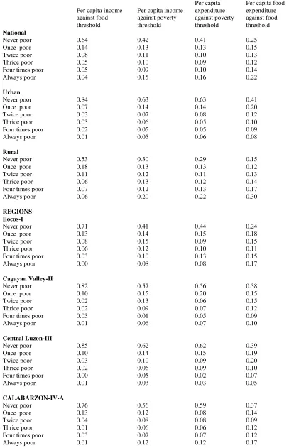
Table 1 presents the DAG chronic and transient components of total poverty for the national level and urban-rural disaggregation. At the national level, chronic poverty is the more substantial component of the total poverty ranging from 84 to 88 per cent of the total poverty. While the transient component ranges between 13 to 23 per cent of the total poverty in urban and rural areas, chronic poverty in rural areas is stable at around 85 per cent regardless of the welfare indicator and threshold used. Urban chronic poverty is lower at 77 per cent when the per capita food expenditure is compared against the food threshold.
2 For details of computation, readers are referred to the National Statistical Coordination Board (NSCB) website,
Based on the per capita food expenditure against the food threshold, NCR has the lowest
total poverty at 11 per cent, 77 per cent of which is attributed to the chronic poverty.3 Central
Luzon and Cagayan Valley also have low total poverty at around 15 to 16 per cent. In the Visayas Island, all regions have roughly the same total poverty at around 19 to 20 per cent, around 84 to 89 per cent is attributed to the chronic poverty. Mindanao Island have the highest total poverty at 24 to 32 per cent. It also has the most regions experiencing high poverty including the regions of CARAGA, ARMM, Zamboanga Peninsula, Davao, Northern Mindanao
and SOCCSKSARGEN4. Regardless of the welfare indicator and threshold used, NCR has the
lowest while CARAGA has the highest chronic poverty
Table 2 presents the mean chronic and transient poverty by characteristics at the household level. The mean chronic poverty is highest for households with heads having no grade completed. It is the lowest for households headed by people with college degree. Results indicate that the mean chronic poverty decreases with the age of the household head. Those headed by people between 18 to 30 years old have the highest while those headed by people above 60 have the lowest mean chronic poverty. Households headed by laborers and unskilled workers and those whose primary occupation is on agriculture, fishery and forestry have the highest mean chronic poverty while households headed by people working as professionals have the lowest mean chronic poverty.
The mean chronic poverty also decreases with the age of the spouse of the household head. Households have high mean chronic poverty when the spouses of the household heads work for private households and without compensation on own family-operated farm/business. Households have low mean chronic poverty when the spouses work for the government or an employer on own family-operated farm/business.
Results show that the mean chronic poverty is higher as the average number of younger members increases. The mean chronic poverty is highest for households with many children between one to 15 years old. Households with fewer members aged over 25 have lower mean chronic poverty, however. While this is the case, the mean chronic poverty of nuclear households is higher than those of extended households. These results are reflective of the findings of Orbeta
(2005) where additional children have regressive impacts on the mother’s earnings and labor
force participation and on the household savings rate. Results on the extended household echo the possibility that risk is shared among adult members.
Aggregate indicator of the household assets is constructed using the score generated by the principal component analysis. The household assets to generate the scores include car, personal computer, air conditioner, gas range, washing machine, refrigerator, television, telephone and radio. A binary variable for each year is created equal to zero for negative scores and one for positive scores. These binary variables are then summed up across the years generating values from zero to five. The value of zero represents households having consistently low socioeconomic status while five represents consistently high status for the five years they are observed. Using the per capita expenditure and poverty threshold, results indicate that households with consistently negative scores in all periods have slightly higher mean chronic
3 Results are not presented but are available upon request from the author.
poverty relative to those with high scores. When the per capita food expenditure is compared against the food threshold, both households have the same mean chronic poverty. The chronic poverty of home owners is lower than non-home owners, on the other hand.
Households that have indicated worse year have the highest mean chronic poverty. Households that have received remittances abroad have the lowest mean chronic poverty while those that have experienced natural calamities and income reduction have the highest chronic poverty. Households have lower chronic poverty when it has a member who has health insurance.
5.EMPIRICAL STRATEY
5.1Chronic and transient poverty
This section analyzes the determinants of poverty components. Following Jalan and Ravallion (2000) to address the many zeros representing the nonpoor, the quantile regression will
be used.5 Briefly, the quantile regression model is formulated as
i i
i i
j
i x Quant y x x
y , ( | ) where yis either the DAG transient or chronic
component and xi is a vector of socioeconomic variables such as the age and education of the
household head, household assets, household composition, geographical dummies to represent
conflict-ridden regions and access to credit and insurance. is the error term associated with a
particular quantile and Quant(yi |xi)xi denotes the th conditional quantile of y. By
using different values of , quantile regression allows the analysis of the relationship of y and
i
x along the different points of the distribution. Quantile regression on the total poverty in the
form of the squared poverty gap will also be implemented.
The regressions will be done using two welfare indicators namely, the per capita expenditure and the per capita food expenditure. The former will be compared against the poverty threshold while the latter will be compared to the food threshold.
5.2 Attrition Bias
Since the research will utilize panel data, there is a need to check for attrition bias. A common issue to the use of any longitudinal data is that the sample collected becomes smaller on succeeding resurvey. This problem becomes serious when non-participants have systematic characteristics that are related to the outcome being investigated. If poor households are more likely to drop out of the succeeding surveys, then estimates based on the remaining samples are likely to be biased. Using these estimates as basis for policy recommendations is likely to raise objections from an empirical standpoint.
Attrition bias is just a case of selection where the sample is limited by the non-participation of survey respondents. Miller and Hollist (2007) argue that attrition bias can affect the external and internal validities of multiwave studies. External validity is questionable when the characteristics of the resulting subsequent samples are not generalizable to the initial samples. Internal validity is questionable when the correlations among the variables are altered
5 As opposed to the tobit approach since this leads to estimators that that are biased in the presence of non-normal
as a result of samples dropping out of the succeeding survey waves. While the NSO has ensured that each replicate of the APIS and FIES possesses the properties of the master sample, we have imposed additional restrictions to ensure that the same families are tracked throughout the periods of observation. These restrictions could be a possible window for attrition bias.
To test for the presence of attrition bias, we follow Miller and Wright (1995) and run a
logit regression on ‘stayers’6
using the independent variables extracted from the first wave. Independent variables include the characteristics of the household head, household assets and geographical location dummies. These dependent variables should not be statistically significant to rule out attrition bias. Result indicates that the characteristics of the household head and some of the regional dummies are statistically significant determinants of participation in the entire
survey wave7. Another method to check for attrition bias is to test for the equality of the two
covariance matrices for the samples observed only in the first period and for the samples observed in all periods using the Box M-test. The null hypothesis using this test is that the two covariance matrices are equal indicating no threats to internal validity. The p-value computed using the Box M-test is 0.00 indicating rejection of the null hypothesis.
Since attrition bias is present in our sample, we follow Heckman (1979) and the inverse
Mills’ Ratio,
) (
) (
x x IMR
, is computed from the probit regression involving the ‘stayers’. IMR
will be included as explanatory variables in the quantile regressions
6.RESULTS AND DISCUSSION
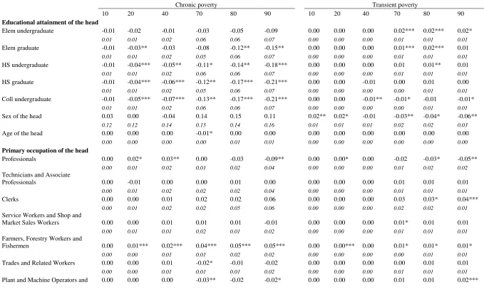
The estimates for the total poverty at various points of distribution are presented in table 3. Panel A contains the estimates from poverty computed using the per capita expenditure and the poverty threshold while panel B presents the estimates from poverty computed using the per capita food expenditure and food threshold. From panel A, the dependent variables do not have explanatory power in the lowest distribution of total poverty but have high explanatory power
from the 40th quantile and above. Results indicate the importance of the educational level of the
household head and its effect varies across the poverty distribution. At the 20th quantile,
households headed by persons with high school units will experience poverty four per cent
lower than households headed by people with no education at all. At the 90th quantile, it is 17
per cent lower. These trends can be observed across the different categories of the highest grade completed but those headed by people with college units have the lowest incidence of
experiencing poverty. At the 20th quantile, those headed by people with college units will
experience poverty six per cent lower than the reference category, 11 per cent lower at the 40th
quantile, 14 per cent lower at the 70th quantile, 15 per cent lower at the 80th quantile and 23 per
cent lower at the 90th quantile. The same trends can be noted in panel B.
From panel A of table 3, households headed by service and market/sales workers and plants/machine operators/assemblers are more likely to experience poverty. Those headed by professionals are more likely to experience poverty than households headed by government
officials and white-collared workers at the lower poverty distribution. At the 80th quantile and above, the trend is reversed. From panel B, households headed by laborers and unskilled workers and by those whose occupations are in the agriculture, fishery and resource sectors experience poverty higher than those headed by government officials and white-collared workers. Like in panel A, households headed by professionals also experience higher poverty at
the lowest distribution. At the 70th quantile, the trend is also reversed. However, it can be seen
that the effect of a professionally-headed households to lower poverty is higher when the basis of poverty computation is the food expenditure food threshold.
From panel A, the household member’s composition based on age categories reveals some points worth emphasizing. Results indicate that households with many young members have higher poverty. Households with many members from one to seven year old have the highest probability followed by households with many members that are less than one year-olds. Those that are composed of many members aged between 15-25 years old also experience higher poverty. Similar findings are noted on panel B as well.
Households with members having health insurance are more relevant in reducing poverty related to food expenditure. Results indicate that these households experience poverty by one to two per cent lower compared to households without. Results in panel A indicate that health insurance is not a significant predictor of poverty with households that experience negative shocks experience higher poverty especially those whose members have lost their jobs. Households receiving remittances abroad have lower poverty relative to households that have not experienced any positive shock.
The effect of remittance is highest on the highest poverty distribution. Better health and increased earnings also lower the poverty but only on selected poverty distribution. When the basis of poverty computation is food expenditure and food threshold, negative shocks do not significantly affect food poverty. Similar to panel A, remittance also negatively affect poverty but its effect is higher in reducing the percentage of experiencing food poverty.
Results also indicate that regions with armed conflicts are more likely to experience poverty. In panel A, households in war-torn regions experience poverty by one to four per cent higher than households in regions without armed conflicts. Households in the rural districts experience poverty by two to eight per cent higher than urban households. The same trends and similar magnitudes can be observed from panel B.
Table 4 presents the estimates of chronic and transient components of poverty computed based on the per capita expenditure and the poverty threshold. The dependent variables do not have explanatory power in the lowest distribution of chronic poverty but have high explanatory
power from the 40th quantile and above. Similar to total poverty, education is also a negative
show that households with more members between zero to one year old have chronic poverty of one to four per cent while those with more members between two to seven year old have chronic poverty of two to seven per cent. Among the negative shocks experienced by the household in 2004, job loss positively and significantly affects the higher chronic poverty distribution. Income reduction is positively and statistically significant in the mid-quantile. Households that receive remittances from abroad have chronic poverty lower by four to eight per cent than households with no positive shocks at all. It should be noted that the effect of remittances can be most felt in the highest quantile of the chronic poverty distribution. Households with at least one member having health insurance experience chronic poverty by one per cent lower than those without. Chronic poverty has a geographical dimension as well. Households in the regions and provinces
that experience armed conflict8 have higher chronic poverty while households in the rural areas
have higher chronic poverty than the urban districts. The effect of rural areas and regions/provinces with armed conflicts on chronic poverty is highest in the highest quantile of the chronic poverty distribution.
The results on transient poverty have a number of differences from the results on chronic poverty. From table 4, the dependent variables explain small variations in the transient poverty
as indicated by the low 2
R in the lower transient poverty distribution. Nine to 13 per cent can be
explained by the dependent variables in the 40th quantile and above. Unlike in the chronic
poverty, results indicate that households headed by people with at least an elementary diploma experience transient poverty by two per cent higher than those headed by people with no education at all. The importance of education to deflect transient poverty can only be observed for households with college units. While most occupations are statistically significant predictor of chronic poverty, professionals are the only occupations to negatively affect transient poverty. Households headed by service and market/sales workers and plant/machine operators have transient poverty that is one per cent higher than the households headed by government officials. Households that have experienced natural disasters such as drought have transient poverty that is three per cent higher than households that have not. Similar to the results on chronic poverty, households that are recipient of remittances from abroad have lower transient poverty but the effect of remittance on chronic poverty is higher. Rural households have higher transient poverty relative to urban households. The IMR is statistically significant, indicating
that the ‘stayers’ have transient poverty higher than the first wave samples only.
Table 5 presents the estimates of chronic and transient components of poverty computed based on the per capita food expenditure and the food threshold. Results have some similarities with table 4. One, the dependent variables do not have explanatory power in the lowest
distribution of chronic poverty. Education negatively affects chronic poverty and its effect is most felt by households headed by people who have college units especially on the highest chronic poverty distribution. Two, the effects of household demographic composition, educational attainment of the household head, job loss and geographic dimension follow the same trend and roughly similar magnitude as in table 4. Similar to table 4, households headed by farmers and workers in the agriculture, fisheries and resource sectors higher chronic poverty experienced by households headed by government officials. The degree of chronic poverty experienced by households headed by farmers and related workers is higher in table 5 where food expenditure and food threshold are the relevant parameters to assess poverty. Better health, increased earnings and remittance ward off chronic poverty arising from food needs. While remittance deflects chronic poverty arising from both food and non-food needs, its effect to lower poverty arising from food needs is higher.
Results on the transient poverty presented in table 5 have similarities in the transient
poverty in table 4 as well. One, the dependent variables explain very little variations in the 10th
quantile and explain around nine per cent in the 20th and 40th quantiles. Two, households headed
by professionals have lower transient poverty but its effect is higher in reducing transient poverty arising from food needs. Households headed by farmers, unskilled workers and plant/machine operators are the ones with higher transient poverty. Three, the effect of natural disasters also follows the same trend and roughly similar magnitude as in table 4. Transient poverty as defined by the food needs does not have geographical dimension. Neither the dummies for regions with conflict nor the urban-rural segregation significantly affects transient poverty in table 5.
7.SUMMARY AND CONCLUSIONS
This paper has attempted to analyze the trends and determinants of chronic and transient poverty in the Philippines. This is one of the few attempts to analyze poverty within the context of dynamic setting. This paper has used the recently developed method of identifying chronic and transient poverty proposed by Duclos, Araar and Giles (2010) and applies it to the 2003 and 2006 FIES and 2004, 2007 and 2008 APIS.
Chronic poverty is the more substantial component accounting for around four/fifths of total poverty at the national level. Households in the rural areas have higher chronic poverty relative to households in the urban districts. At the regional level, NCR has the lowest and CARAGA has the highest chronic poverty. Mindanao Island also has the most regions to have high chronic poverty. Simple cross-tabulations indicate that the mean chronic poverty is higher for households headed by people 18-30 years old, with no educational level completed or who are laborers and whose primary occupations are on the agriculture, fisheries and resource sectors. Households with many children and those that experienced negative shocks like drought and income reduction have high mean chronic poverty as well.
Based on the results from the quantile regressions, the dependent variables have low
explanatory power at the lowest poverty distribution but can explain significant variations from
the 40th quantile and above. In addition, total poverty and chronic poverty can be explained by
location. These variables can explain significant variations in the total poverty and total chronic poverty. While the signs are generally maintained, these variables either are insignificant or explain fewer variations in the total transient poverty.
Nevertheless, there are still some interesting results from the contrast between chronic and transient poverty. One, while education at all levels deflects chronic poverty, results indicate that transient poverty is higher for educational levels lower than college. This is possibly because educational attainment can dictate the types of work arrangements one will do in the labor market. For example, seasonal or temporary workers are typically those that are at most high school graduate. To the extent that these types of workers are not protected by contracts, slack
seasons can lead to substantial variations on the person’s ability to meet the food and non-food
basic needs of their households.
In addition, chronic and transient poverty are affected by different sets of shocks. Negative shocks related to the labor market, such as job loss or income reduction, increases chronic poverty while natural disasters, such as drought, increase transient poverty. This is possibly due to the fact that once retrenched, workers are faced by unemployment that may be prolonged depending on the state of the economy and the needs of the labor market. Job search
coupled by employer’s screening efforts will also lengthen the time of unemployment. Although
crippling, shocks originating from natural disasters can have immediate solutions through adequate provisions of infrastructure such as irrigation or deep-well water supply in cases of drought. Once infrastructures are correctly in place, households that are affected by the shock will be able to restore their capacity to meet their basic needs.
The paper also uses two ways in which the DAG poverty is computed: the per capita expenditure compared against the poverty threshold and the per capita food expenditure versus the food threshold. Regardless of the welfare indicator and the threshold used, results show that households headed by farmers and related-workers and by unskilled workers experience higher chronic poverty. However, chronic poverty arising from food needs is higher when the households are headed by people in these types of occupations. There are also more positive shocks, such as better health, increased earnings and remittance, which affect chronic poverty arising from food needs while chronic poverty arising from food and non-food basic needs is affected by remittance only. It can be noted that remittance lowers chronic poverty related to food needs more than it lowers chronic poverty related to both food and non-food basic needs. This is consistent with the findings of studies that to some extent, remittances are used to smooth consumption.
Results indicate that policies to address chronic and transient poverty require different targets. In the case of the Philippines, chronic poverty is the more substantial portion of the total
poverty and therefore requires more emphasis in the government’s efforts to eliminate poverty. This result echoes Duclos, Araar and Giles (2010) findings in China where transient poverty only accounts for around 23 per cent of the total poverty. To address chronic poverty, social safety nets should be in place to tackle negative shocks stemming from the labor market. This requires a more structural approach in the sense that the government should not only provide primary education to all but to ensure school progression especially in rural areas where chronic poverty
conditions that aim to provide long-run solutions to poverty and the government should complement this by providing adequate school and health infrastructures and facilities to ensure
that the program’s conditions are met. Two, social protection should be sustainable in the long
-run. This is an anti-poverty program that is growing in cost annually to meet the MDG commitment to reduce poverty by year 2015 and requires increasingly huge amount that can only be sustained by a well-functioning fiscal system and a wider tax base.
Strong link between developing technical/vocational skills and local livelihood opportunities is also needed to ensure that high school graduates who will not be able to afford college education will be equipped with skills that are valuable in the labor market. In this context, the government is highly commendable for establishing the Technical Education and Skills Development Authority. To sustain low poverty in the long-run, strong link between the academe and the industry is needed to ensure that the courses being offered in colleges and universities are relevant to the needs of the local labor market. Industries that have the potential to generate high value-added and job opportunities should be identified and developed to ensure continuous income stream.
Consistent with the findings in the literature (Bhide and Mehta, 2004; Herrera and Roubaud, 2005), results indicate that the higher number of dependent children positively affects chronic poverty but not transient poverty. This calls for a strong population and reproductive health program. While there is an effort to address the increasing population in the Philippines through the Reproductive Health (RH) Bill, it is still undergoing legislative deliberations and public debates and discourses that reflect the divided sentiments of the different sectors in the economy. In a nutshell, the RH Bill promotes the use of all family planning methods and age-appropriate sex education. Despite the volume of research that emphasizes the disadvantageous effect of an unchecked growing population, those opposed to the RH Bill find support from the religious teachings to value life. They also find support from economic researches conducted by well-respected international economist showing increased premarital sex and extramarital affairs among other social maladies resulting from the use of contraceptives. However, evidence closer to home should not be ignored such as Orbeta (2005, 2003) and the findings of the research at hand. At the minimum, the government should not be constrained to provide all the set of information necessary to make parents/adults responsible in the reproductive arena. Rather than an impasse, all concerned sectors should agree on the acceptable responsible parenthood practices that the government can integrate in their delivery of social health service.
References
Aldaba, F. (2009). Poverty in the Philippines: Causes, consequences and opportunities. ADB Report. Manila: Asian Development Bank.
Antolin, P., T. Dang and H. Oxley (1999). Poverty dynamics in four OECD countries. OECD Economics Department Working Paper No. 212. France: Organisation for Economic Co-operation and Development.
Balisacan, A. and H. Hill (2003). The Philippine economy: Development, policies, and challenges. New York: Oxford University Press.
Balisacan, A. (2003). Poverty comparison in the Philippines: Is what we know about the poor robust? In C. Edmonds (ed.). Reducing poverty in Asia: Emerging issues in growth, targeting, and measurement. Cheltenham, UK: Edward Elgar.
Balisacan, A. and E. Pernia, (2002). The rural road to poverty reduction: Some lessons from the Philippine experience, Journal of Asian and African Studies. 37(2), pp. 147-167.
Bhide, S. and A. Mehta (2004). Chronic poverty in Rural India: Issues and findings from panel data. Journal of Human Development, 5(2), pp. 195-209.
Devicienti, F. (2002). Estimating poverty persistence in Britain. CES Working Paper Series No. 1. Italy: Centre for Employment Studies.
Duclos, J., A. Araar, and J. Giles (2010). Chronic and transient poverty: Measurement and estimation, with evidence from China. Journal of Development Economics, 91(2), pp. 266-277.
Duncan, G. and W. Rodgers (1991). Has children’s poverty become more persistent? American Sociological Review. 56(4), pp. 538-550.
Finnie, R. and A. Sweetman (2003). Poverty dynamics: Empirical evidence for Canada. The Canadian Journal of Economics, 36(2), pp. 291-325.
Foster, J., J. Greer and E. Thorbecke (1984). A class of decomposable poverty measures. Econometrica, 52(3), pp. 761–765.
Haddad, L. and A. Ahmed (2003). Chronic and transitory poverty: Evidence for Egypt, 1997-99. World Development, 31(1), pp. 71-85.
Heckman, J. (1979). Sample selection bias as a specification error. Econometrica, 47(1), pp. 153–161.
Herrera, J. and F. Roubaud (2005). Urban poverty dynamics in Peru and Madagascar, 1997-99: A Panel Data Analysis. International Planning Studies, 10(1), pp. 21–48.
Jalan, J. and M. Ravallion (1998). Transient poverty in postreform Rural China. Journal of Comparative Economics, 26(2), pp. 338-357.
Jalan, J. and M Ravallion (2000). Is transient poverty different? Evidence for Rural China. Journal of Development Studies, 36(6), pp. 82-100.
Jenkins, S., C. Schluter and G. Wagner (2003). The dynamics of child poverty in Britain and Germany compared. Journal of Comparative Family Studies, 34(3), pp. 337-353.
Lillard, L. and R. Willis (1978). Dynamic aspects of earnings mobility. Econometrica, 46(5), pp. 985-1012.
McCulloch, N. and B. Baulch (2000). Simulating the impact of policy upon chronic and transient poverty in Rural Pakistan. Journal of Development Studies, 36(6), pp. 100-130.
Miller, R. and C. Hollist (2007). Attrition bias. In N. Salkind (ed.). Encyclopedia of measurement and statistics, 3 volumes (57-60). Thousand Oaks: Sage Reference.
Miller, R. and W. Wright (1995). Detecting and correcting attrition bias in longitudinal family research. Journal of Marriage and Family, 57(4), pp. 921-929.
Orbeta, A. (2005). Poverty, vulnerability and family size: Evidence from the Philippines. PIDS Discussion Paper Series No. 2005-19. Manila: Philippine Institute for Development Studies.
Orbeta, A. (2003). Population and poverty: A review of the evidence, links, implications for the Philippines. Philippine Journal of Development, XXX(2), pp. 198–227.
Table 1: Proportion of households moving in and out of poverty for the 5-year period, APIS and FIES
Per capita income against food threshold
Per capita income against poverty threshold Per capita expenditure against poverty threshold
Per capita food expenditure against food threshold National
Never poor 0.64 0.42 0.41 0.25
Once poor 0.14 0.13 0.13 0.15
Twice poor 0.08 0.11 0.10 0.13
Thrice poor 0.05 0.10 0.09 0.12
Four times poor 0.05 0.09 0.10 0.14
Always poor 0.04 0.15 0.16 0.22
Urban
Never poor 0.84 0.63 0.63 0.41
Once poor 0.07 0.14 0.14 0.20
Twice poor 0.03 0.07 0.08 0.12
Thrice poor 0.03 0.06 0.05 0.10
Four times poor 0.02 0.05 0.05 0.09
Always poor 0.01 0.05 0.06 0.08
Rural
Never poor 0.53 0.30 0.29 0.15
Once poor 0.18 0.13 0.13 0.12
Twice poor 0.11 0.12 0.11 0.13
Thrice poor 0.06 0.13 0.12 0.14
Four times poor 0.07 0.12 0.13 0.17
Always poor 0.06 0.20 0.22 0.30
REGIONS Ilocos-I
Never poor 0.71 0.41 0.44 0.24
Once poor 0.13 0.14 0.15 0.18
Twice poor 0.08 0.15 0.09 0.15
Thrice poor 0.06 0.12 0.10 0.11
Four times poor 0.03 0.10 0.13 0.15
Always poor 0.00 0.08 0.08 0.17
Cagayan Valley-II
Never poor 0.82 0.57 0.56 0.38
Once poor 0.10 0.15 0.20 0.15
Twice poor 0.02 0.13 0.06 0.15
Thrice poor 0.02 0.09 0.07 0.12
Four times poor 0.03 0.01 0.05 0.09
Always poor 0.01 0.06 0.07 0.10
Central Luzon-III
Never poor 0.85 0.62 0.62 0.39
Once poor 0.10 0.14 0.15 0.19
Twice poor 0.03 0.10 0.09 0.20
Thrice poor 0.02 0.06 0.09 0.10
Four times poor 0.00 0.05 0.02 0.07
Always poor 0.01 0.03 0.03 0.05
CALABARZON-IV-A
Never poor 0.76 0.56 0.59 0.37
Once poor 0.13 0.12 0.08 0.14
Twice poor 0.04 0.08 0.08 0.09
Thrice poor 0.01 0.06 0.06 0.12
Four times poor 0.03 0.07 0.07 0.12
MIMAROPA-IV-B
Never poor 0.48 0.29 0.29 0.13
Once poor 0.20 0.13 0.10 0.10
Twice poor 0.14 0.13 0.14 0.11
Thrice poor 0.08 0.12 0.11 0.14
Four times poor 0.06 0.14 0.11 0.20
Always poor 0.05 0.20 0.26 0.33
Bicol-V
Never poor 0.31 0.31 0.33 0.17
Once poor 0.16 0.16 0.12 0.17
Twice poor 0.10 0.10 0.13 0.17
Thrice poor 0.12 0.12 0.10 0.06
Four times poor 0.13 0.13 0.12 0.23
Always poor 0.19 0.19 0.20 0.21
Western Visayas-VI
Never poor 0.70 0.43 0.43 0.26
Once poor 0.12 0.14 0.13 0.16
Twice poor 0.05 0.08 0.09 0.10
Thrice poor 0.02 0.14 0.12 0.13
Four times poor 0.07 0.06 0.09 0.12
Always poor 0.03 0.15 0.15 0.23
Central Visayas-VII
Never poor 0.61 0.41 0.40 0.24
Once poor 0.21 0.19 0.18 0.17
Twice poor 0.08 0.12 0.08 0.13
Thrice poor 0.04 0.11 0.11 0.14
Four times poor 0.06 0.10 0.14 0.13
Always poor 0.01 0.06 0.10 0.19
Eastern Visayas-VIII
Never poor 0.56 0.38 0.34 0.23
Once poor 0.23 0.15 0.14 0.13
Twice poor 0.04 0.09 0.16 0.14
Thrice poor 0.05 0.15 0.11 0.11
Four times poor 0.09 0.07 0.10 0.19
Always poor 0.03 0.15 0.15 0.21
Zamboanga Peninsula-IX
Never poor 0.51 0.30 0.29 0.16
Once poor 0.11 0.17 0.13 0.15
Twice poor 0.06 0.08 0.10 0.11
Thrice poor 0.09 0.06 0.03 0.13
Four times poor 0.08 0.07 0.11 0.08
Always poor 0.16 0.33 0.35 0.38
Northern Mindanao-X
Never poor 0.57 0.38 0.34 0.19
Once poor 0.11 0.15 0.17 0.13
Twice poor 0.10 0.07 0.10 0.12
Thrice poor 0.07 0.09 0.05 0.12
Four times poor 0.05 0.07 0.11 0.13
Always poor 0.09 0.25 0.24 0.30
Davao-XI
Never poor 0.54 0.35 0.32 0.15
Once poor 0.12 0.10 0.11 0.14
Thrice poor 0.06 0.10 0.12 0.21
Four times poor 0.07 0.18 0.16 0.15
Always poor 0.05 0.18 0.20 0.24
SOCCSKSARGEN-XII
Never poor 0.54 0.39 0.36 0.22
Once poor 0.14 0.10 0.15 0.12
Twice poor 0.15 0.13 0.10 0.15
Thrice poor 0.07 0.08 0.09 0.12
Four times poor 0.07 0.12 0.09 0.14
Always poor 0.04 0.17 0.20 0.25
National Capital Region
Never poor 0.99 0.79 0.76 0.56
Once poor 0.01 0.11 0.13 0.21
Twice poor 0.04 0.06 0.12
Thrice poor 0.04 0.03 0.06
Four times poor 0.02 0.02 0.03
Always poor 0.00 0.01
Cordillera Administrative Region
Never poor 0.54 0.34 0.07 0.09
Once poor 0.22 0.15 0.09 0.16
Twice poor 0.15 0.14 0.11 0.12
Thrice poor 0.04 0.18 0.25 0.18
Four times poor 0.02 0.11 0.32 0.19
Always poor 0.02 0.08 0.16 0.26
Autonomous Region of Muslim Mindanao
Never poor 0.48 0.08 0.05 0.03
Once poor 0.21 0.08 0.13 0.05
Twice poor 0.12 0.23 0.12 0.07
Thrice poor 0.12 0.24 0.23 0.17
Four times poor 0.05 0.19 0.21 0.29
Always poor 0.02 0.19 0.26
CARAGA-XIII
Never poor 0.33 0.16 0.17 0.06
Once poor 0.16 0.10 0.12 0.10
Twice poor 0.16 0.12 0.11 0.10
Thrice poor 0.14 0.12 0.12 0.14
Four times poor 0.08 0.16 0.13 0.15
Table 2: Total poverty and its components at the national level and at the urban-rural segregation using JR and DAG approach
1 2 3 4
Per capita income against food threshold
Per capita income against poverty threshold
Per capita food expenditure against poverty threshold
Per capita expenditure against food threshold
National Obs JR DAG % of DAG total
poverty Obs JR DAG
% of DAG total
poverty Obs JR DAG
% of DAG total
poverty Obs JR DAG
% of DAG total poverty
Total Poverty 915 0.05 0.22 1502 0.08 0.29 2571 0.04 0.21 1940 0.08 0.28
Total Chronic 0.02 0.16 0.75 0.05 0.24 0.82 0.03 0.18 0.88 0.05 0.23 0.84
Total Transient 0.03 0.05 0.25 0.03 0.05 0.18 0.01 0.03 0.12 0.03 0.05 0.16
Urban
Total Poverty 143 0.03 0.19 343 0.05 0.23 920 0.02 0.13 539 0.05 0.21
Total Chronic 0.01 0.14 0.73 0.03 0.18 0.78 0.01 0.11 0.87 0.02 0.17 0.77
Total Transient 0.02 0.05 0.27 0.03 0.05 0.22 0.01 0.02 0.13 0.02 0.05 0.23
Rural
Total Poverty 772 0.05 0.22 1159 0.09 0.30 1171 0.08 0.28 1401 0.09 0.30
Total Chronic 0.02 0.17 0.76 0.06 0.25 0.83 0.06 0.24 0.85 0.06 0.25 0.85
Table 3: Total poverty and its components at the regional level using DAG approach
1 2 3 4
Per capita income against
food threshold
Per capita income against poverty
threshold
Per capita expenditure against
poverty threshold
Per capita food expenditure against food threshold Obs DAG poverty components
% of total poverty
DAG poverty components
% of total poverty
DAG poverty components
% of total poverty DAG poverty components % of total poverty Ilocos-I
Total Poverty 160 0.04 0.18 0.16 0.2
Total Chronic 0.02 0.62 0.15 0.83 0.14 0.84 0.16 0.83
Total Transient 0.01 0.38 0.03 0.17 0.03 0.16 0.03 0.17
Cagayan Valley-II
Total Poverty 163 0.02 0.13 0.12 0.16
Total Chronic 0.01 0.64 0.11 0.85 0.11 0.87 0.13 0.83
Total Transient 0.01 0.36 0.02 0.15 0.02 0.13 0.03 0.17
Central Luzon-III
Total Poverty 191 0.02 0.12 0.1 0.15
Total Chronic 0.01 0.58 0.1 0.83 0.08 0.82 0.12 0.78
Total Transient 0.01 0.42 0.02 0.17 0.02 0.18 0.03 0.22
CALABARZON-IVA
Total Poverty 275 0.02 0.16 0.16 0.2
Total Chronic 0.02 0.64 0.15 0.9 0.14 0.9 0.18 0.88
Total Transient 0.01 0.36 0.02 0.1 0.02 0.1 0.03 0.12
MIMAROPA-IVB
Total Poverty 133 0.08 0.26 0.24 0.28
Total Chronic 0.06 0.67 0.22 0.85 0.21 0.87 0.24 0.86
Total Transient 0.03 0.33 0.04 0.15 0.03 0.13 0.04 0.14
Bicol-V
Total Poverty 205 0.07 0.24 0.21 0.25
Total Chronic 0.05 0.69 0.2 0.86 0.19 0.86 0.21 0.85
Total Transient 0.02 0.31 0.03 0.14 0.03 0.14 0.04 0.15
Western Visayas-VI
Total Poverty 220 0.05 0.2 0.19 0.23
Total Chronic 0.04 0.72 0.18 0.88 0.17 0.89 0.2 0.87
Total Transient 0.01 0.28 0.02 0.12 0.02 0.11 0.03 0.13
Central Visayas-VII
Total Poverty 125 0.06 0.2 0.2 0.25
Total Chronic 0.04 0.66 0.17 0.83 0.17 0.85 0.21 0.84
Total Transient 0.02 0.34 0.03 0.17 0.03 0.15 0.04 0.16
Eastern Visayas-VIII
Total Poverty 123 0.08 0.23 0.21 0.25
Total Chronic 0.05 0.69 0.19 0.84 0.18 0.85 0.22 0.87
Total Transient 0.02 0.31 0.04 0.16 0.03 0.15 0.03 0.13
Zamboanga Peninsula-IX
Total Poverty 104 0.13 0.33 0.31 0.32
Total Chronic 0.11 0.82 0.3 0.91 0.28 0.91 0.29 0.89
Northern Mindanao-X
Total Poverty 151 0.09 0.27 0.26 0.29
Total Chronic 0.07 0.76 0.24 0.89 0.23 0.89 0.26 0.88
Total Transient 0.02 0.24 0.03 0.11 0.03 0.11 0.03 0.12
Davao-XI
Total Poverty 136 0.1 0.27 0.26 0.29
Total Chronic 0.07 0.68 0.23 0.85 0.22 0.85 0.24 0.83
Total Transient 0.03 0.32 0.04 0.15 0.04 0.15 0.05 0.17
SOCCSKSARGEN-XII
Total Poverty 106 0.07 0.23 0.21 0.24
Total Chronic 0.05 0.68 0.2 0.87 0.18 0.88 0.2 0.86
Total Transient 0.02 0.32 0.03 0.13 0.03 0.12 0.03 0.14
National Capital Region
Total Poverty 141 0 0.06 0.06 0.11
Total Chronic 0 0.45 0.05 0.82 0.05 0.82 0.08 0.77
Total Transient 0 0.55 0.01 0.18 0.01 0.18 0.02 0.23
Cordillera Administrative Region
Total Poverty 85 0.07 0.24 0.23 0.27
Total Chronic 0.05 0.62 0.19 0.8 0.19 0.82 0.22 0.83
Total Transient 0.03 0.38 0.05 0.2 0.04 0.18 0.05 0.17
Autonomous Region of Muslim Mindanao
Total Poverty 118 0.06 0.23 0.22 0.29
Total Chronic 0.04 0.62 0.19 0.81 0.19 0.84 0.25 0.86
Total Transient 0.02 0.38 0.04 0.19 0.04 0.16 0.04 0.14
CARAGA-XIII
Total Poverty 135 0.14 0.33 0.31 0.34
Total Chronic 0.11 0.75 0.29 0.88 0.27 0.88 0.3 0.87
Table 4: Mean chronic and transient poverty using DAG approach, by socioeconomic characteristics
1 2 3 4
Per capita income against food threshold Per capita income against poverty threshold Per capita expenditure against poverty threshold
Per capita food expenditure against food threshold Educational Attainment of the household head (FIES 2003)
No grade completed 0.12 0.03 0.12 0.03 0.24 0.03 0.3 0.03
Elem undergraduate 0.08 0.03 0.08 0.03 0.17 0.04 0.21 0.04
Elem graduate 0.05 0.02 0.05 0.02 0.13 0.03 0.18 0.04
HS undergraduate 0.04 0.02 0.04 0.02 0.1 0.03 0.14 0.04
HS graduate 0.02 0.01 0.02 0.01 0.07 0.02 0.11 0.03
College undergraduate 0.02 0.01 0.02 0.01 0.04 0.01 0.07 0.02
Age of the household head (FIES 2003)
Between 18 to 30 0.06 0.02 0.06 0.02 0.14 0.03 0.18 0.04
Between 31 to 40 0.06 0.02 0.06 0.02 0.14 0.03 0.17 0.03
Between 41 to 50 0.03 0.02 0.03 0.02 0.09 0.02 0.14 0.03
Between 51 to 60 0.03 0.01 0.03 0.01 0.08 0.02 0.12 0.03
Above 60 0.02 0.01 0.02 0.01 0.06 0.02 0.09 0.03
Primary occupation of the household head (FIES 2003)
Special Occupations 0.03 0 0.03 0 0.08 0.02 0.14 0.03
Officials of Government and Special-Interest
Organizations, Corporate Executives, Managers, Managing Proprietors and
Supervisors 0.01 0 0.01 0 0.03 0.01 0.05 0.02
Professionals 0 0 0 0 0 0 0.02 0.01
Technicians and Associate
Professionals 0 0 0 0 0.02 0.01 0.05 0.02
Clerks 0.01 0.01 0.01 0.01 0.04 0.02 0.05 0.03
Service Workers and Shop
and Market Sales Workers 0.02 0.01 0.02 0.01 0.06 0.02 0.1 0.03
Farmers, Forestry Workers
and Fishermen 0.07 0.03 0.07 0.03 0.15 0.03 0.19 0.04
Trades and Related Workers 0.02 0.01 0.02 0.01 0.07 0.02 0.11 0.03
Plant and Machine Operators
and Assemblers 0.02 0.01 0.02 0.01 0.06 0.02 0.1 0.04
Laborers and Unskilled
Workers 0.06 0.02 0.06 0.02 0.15 0.03 0.19 0.04
Age of the spouse (APIS 2004)
Between 18 to 30 0.06 0.03 0.06 0.03 0.15 0.04 0.19 0.04
Between 31 to 40 0.06 0.02 0.06 0.02 0.14 0.03 0.18 0.03
Between 41 to 50 0.05 0.02 0.05 0.02 0.11 0.03 0.15 0.04
Between 51 to 60 0.03 0.02 0.03 0.02 0.08 0.02 0.12 0.03
Above 60 0.02 0.01 0.02 0.01 0.05 0.02 0.08 0.03
Class of work of spouse (APIS 2004)
Worked for private household 0.06 0.02 0.06 0.02 0.14 0.03 0.18 0.04
Worked for private
establishment 0.05 0.02 0.05 0.02 0.12 0.03 0.15 0.03
Worked for gov't/gov't corp 0.02 0.01 0.02 0.01 0.05 0.02 0.09 0.02
Self Employed w/out any
employee 0.04 0.02 0.04 0.02 0.1 0.03 0.14 0.03
Employer in own family
operated farm or business 0.01 0 0.01 0 0.02 0.01 0.05 0.02
family operated farm or business
Worked w/out pay on own family operated farm or
business 0.07 0.03 0.07 0.03 0.14 0.03 0.17 0.04
Mean number of household members aged <=1 yo (APIS and FIES)
0 0.03 0.02 0.03 0.02 0.09 0.02 0.13 0.03
Between 0 and 1 0.08 0.03 0.08 0.03 0.16 0.03 0.2 0.04
Between 1 and 2 0.1 0.01 0.1 0.01 0.18 0.03 0.22 0.04
Mean number of household members aged <=7 yo (APIS and FIES)
0 0.02 0.01 0.02 0.01 0.05 0.02 0.09 0.03
Between 0 and 1 0.04 0.02 0.04 0.02 0.1 0.03 0.14 0.04
Between 1 and 2 0.08 0.03 0.08 0.03 0.18 0.03 0.22 0.04
Between 2 and 3 0.14 0.04 0.14 0.04 0.26 0.04 0.3 0.04
Between 3 and 4 0.15 0.05 0.15 0.05 0.34 0.04 0.38 0.03
Between 4 and 5 0.23 0.07 0.23 0.07 0.33 0.07 0.29 0.07
Mean number of household members aged <=15 (APIS and FIES)
0 0.02 0.01 0.02 0.01 0.05 0.02 0.08 0.03
Between 0 and 1 0.03 0.02 0.03 0.02 0.07 0.03 0.11 0.04
Between 1 and 2 0.05 0.02 0.05 0.02 0.13 0.03 0.17 0.04
Between 2 and 3 0.1 0.03 0.1 0.03 0.2 0.03 0.25 0.04
Between 3 and 4 0.13 0.04 0.13 0.04 0.26 0.04 0.31 0.03
Between 4 and 5 0.13 0.03 0.13 0.03 0.26 0.03 0.31 0.03
Mean number of household members aged <25 (APIS and FIES)
0 0.05 0.02 0.05 0.02 0.11 0.02 0.14 0.03
Between 0 and 1 0.04 0.02 0.04 0.02 0.1 0.03 0.14 0.03
Between 1 and 2 0.04 0.02 0.04 0.02 0.1 0.03 0.14 0.04
Between 2 and 3 0.05 0.02 0.05 0.02 0.12 0.03 0.17 0.04
Between 3 and 4 0.04 0.02 0.04 0.02 0.11 0.03 0.17 0.04
Mean number of household members aged >25 (APIS and FIES)
0 0.07 0.02 0.07 0.02 0.16 0.03 0.23 0.03
Between 0 and 1 0.05 0.02 0.05 0.02 0.11 0.03 0.15 0.03
Between 1 and 2 0.03 0.02 0.03 0.02 0.08 0.02 0.12 0.03
Between 2 and 3 0.01 0.01 0.01 0.01 0.05 0.02 0.09 0.03
Between 3 and 4 0.02 0.02 0.02 0.02 0.07 0.02 0.12 0.04
Changes in the type of household (APIS and FIES)
Nuclear all 5 periods 0.05 0.02 0.05 0.02 0.12 0.03 0.15 0.03
Once extended 0.05 0.02 0.05 0.02 0.1 0.03 0.14 0.04
Twice extended 0.04 0.02 0.04 0.02 0.1 0.03 0.14 0.03
Thrice extended 0.03 0.02 0.03 0.02 0.08 0.03 0.12 0.04
Four times extended 0.03 0.02 0.03 0.02 0.08 0.02 0.13 0.03
Extended all 5 periods 0.02 0.01 0.02 0.01 0.07 0.02 0.11 0.03
Changes in home ownership (APIS) No change in hh ownership:
does not own in 3 periods 0.04 0.02 0.04 0.02 0.11 0.03 0.15 0.03
Owned once 0.05 0.02 0.05 0.02 0.09 0.02 0.12 0.03
Owned twice 0.02 0.01 0.02 0.01 0.05 0.01 0.09 0.03
No change in hh ownership:
own in 3 periods 0 0 0 0 0.03 0.01 0.08 0.02
Without parents in the 3-yr pd 0.04 0.02 0.04 0.02 0.1 0.03 0.14 0.03
With parents in the 3-yr pd 0.05 0.02 0.05 0.02 0.11 0.03 0.15 0.04
Change in asset ownership (PCA score using APIS and FIES)
Low score in all periods 0.01 0.01 0.01 0.01 0.04 0.02 0.09 0.04
High score once 0.02 0.01 0.02 0.01 0.07 0.03 0.12 0.04
High score twice 0.07 0.03 0.07 0.03 0.16 0.03 0.2 0.04
High score thrice 0 0 0 0 0.02 0.01 0.04 0.02
High score four times 0.01 0.01 0.01 0.01 0.04 0.02 0.09 0.04
High score in all periods 0.02 0.02 0.02 0.02 0 0 0.09 0.05
Changes in welfare (APIS 2004)
Better-off 0.04 0.02 0.04 0.02 0.09 0.02 0.12 0.03
Worse-off 0.05 0.02 0.05 0.02 0.12 0.03 0.16 0.04
The same 0.04 0.02 0.04 0.02 0.1 0.03 0.14 0.03
Positive shocks (APIS 2004)
New job with higher salary 0.03 0.02 0.03 0.02 0.08 0.03 0.11 0.04
Abundant harvest 0.07 0.03 0.07 0.03 0.13 0.03 0.16 0.03
Better Health 0.02 0.02 0.02 0.02 0.06 0.02 0.1 0.03
More Earnings 0.04 0.02 0.04 0.02 0.09 0.02 0.13 0.03
More Remittances Abroad 0 0.01 0 0.01 0.01 0.01 0.03 0.02
Inheritance 0 0 0 0 0.05 0.07 0.07 0.09
Others 0.06 0.03 0.06 0.03 0.12 0.03 0.16 0.04
Negative shocks (APIS 2004)
Lost Job/Work 0.04 0.02 0.04 0.02 0.11 0.03 0.15 0.04
Natural Disaster, Drought 0.08 0.05 0.08 0.05 0.16 0.05 0.19 0.05
Increased Food Prices 0.04 0.02 0.04 0.02 0.11 0.03 0.15 0.04
Poor Health 0.04 0.01 0.04 0.01 0.09 0.03 0.13 0.03
Reduced Income 0.07 0.02 0.07 0.02 0.14 0.03 0.18 0.04
No Savings 0.04 0.02 0.04 0.02 0.1 0.02 0.15 0.03
Others 0.03 0.02 0.03 0.02 0.1 0.02 0.14 0.03
Any one in the household member with health insurance (APIS 2004)
No one 0.05 0.02 0.05 0.02 0.12 0.03 0.16 0.04
Table 5: Check for attrition bias using logit on the “stayers”
Coef. Std. Err. P>|z|
Age, household head -0.01 0.00 0.00
Sex, household head -2.63 0.53 0.00
Urban 0.09 0.07 0.21
Region II 0.17 0.18 0.32
Region III -0.21 0.16 0.19
Region V 0.67 0.18 0.00
Region VI 0.25 0.16 0.13
Region VII -0.45 0.17 0.01
Region VIII -0.22 0.18 0.22
Region IX -0.22 0.19 0.25
Region X 0.43 0.19 0.02
Region XI 0.00 0.19 0.98
Region XII -0.31 0.18 0.09
Region XIII -0.15 0.18 0.42
Region XIV -0.11 0.20 0.57
Region XV -0.29 0.18 0.11
Region XVI 0.51 0.19 0.01
Region IV-A 0.45 0.16 0.01
Region IV-B 0.20 0.19 0.28
Number of members aged up to 1 yo -0.03 0.10 0.74
Number of members aged up to 7 yo -0.09 0.04 0.01
Number of members aged up to 15 yo -0.03 0.03 0.19
Number of members aged up to 25 yo -0.04 0.03 0.15
Number of members aged greater than 25 yo -0.03 0.04 0.51
Owned radio -0.03 0.07 0.63
Owned TV -0.06 0.08 0.49
Owned Ref -0.11 0.09 0.22
Owned Washing machine -0.17 0.10 0.08
Owned Aircon -0.19 0.17 0.26
Constant 4.68 0.67 0.00
LR Chi^2 204.19
Prob>Chi^2 -2963.25
Pseudo R^2 0.03
Number of observations 2251
Table 6: Quantile regression estimates on total poverty based on DAG approach
Panel A Panel B
Per capita expenditure against poverty threshold Per capita food expenditure against food threshold
10 20 40 70 80 90 10 20 40 70 80 90
Educational attainment of the head
Elem undergraduate -0.02 -0.01 -0.01 -0.02 -0.03 -0.08 -0.07*** -0.07*** -0.03* 0.00 -0.04 -0.07
0.02 0.02 0.02 0.04 0.04 0.06 0.02 0.02 0.02 0.03 0.03 0.05
Elem graduate -0.02 -0.03 -0.04* -0.06 -0.09* -0.13** -0.09*** -0.10*** -0.06*** -0.04 -0.07*** -0.11*
0.02 0.02 0.02 0.05 0.05 0.06 0.02 0.02 0.02 0.03 0.03 0.06
HS undergraduate -0.02 -0.04** -0.07*** -0.10** -0.10*** -0.17*** -0.10*** -0.11*** -0.09*** -0.07* -0.10*** -0.15***
0.02 0.02 0.02 0.04 0.04 0.06 0.03 0.02 0.02 0.04 0.03 0.06
HS graduate -0.03 -0.05** -0.08*** -0.12*** -0.14*** -0.19*** -0.11*** -0.14*** -0.11*** -0.09*** -0.12*** -0.16***
0.02 0.02 0.02 0.04 0.04 0.06 0.03 0.02 0.02 0.03 0.03 0.06
Coll undergraduate -0.03* -0.06*** -0.11*** -0.14*** -0.15*** -0.23*** -0.13*** -0.16*** -0.14*** -0.12*** -0.16*** -0.20***
0.02 0.02 0.02 0.04 0.04 0.06 0.02 0.02 0.02 0.04 0.03 0.05
Sex of the head 0.06 0.01 -0.03 0.12 0.10 0.16 0.11* 0.04 -0.03 0.06 0.05 0.01
0.11 0.12 0.13 0.14 0.14 0.14 0.06 0.04 0.10 0.11 0.11 0.11
Age of the head 0.00 0.00 0.00 -0.01 0.00 0.00 0.00 0.01* 0.00 0.00 -0.01 0.00
0.00 0.00 0.01 0.01 0.01 0.01 0.00 0.00 0.00 0.01 0.01 0.00 Primary occupation of the head
Professionals 0.00 0.03* 0.04* -0.02 -0.07* -0.12** 0.05* 0.04 -0.01 -0.09** -0.12** -0.18*
0.01 0.02 0.02 0.02 0.04 0.06 0.03 0.03 0.01 0.05 0.06 0.10 Technicians and Associate
Professionals 0.00 -0.02 0.00 0.00 0.00 0.02 -0.03 0.01 0.00 0.00 0.03 0.04
0.00 0.02 0.02 0.03 0.03 0.03 0.03 0.03 0.02 0.03 0.04 0.05
Clerks 0.00 0.00 0.02 0.03 0.03 0.03 0.01 0.01 0.01 0.02 0.04 0.03
0.00 0.02 0.03 0.03 0.04 0.08 0.03 0.03 0.04 0.05 0.05 0.05 Service Workers and Shop and
Market Sales Workers 0.00 0.01 0.01 0.01 0.00 -0.01 0.01 0.03 0.03 0.04* 0.04 0.02
0.00 0.01 0.02 0.02 0.02 0.02 0.01 0.02 0.02 0.02 0.02 0.03 Farmers, Forestry Workers and
Fishermen 0.00 0.02*** 0.03** 0.05*** 0.06*** 0.07*** 0.03*** 0.04*** 0.04*** 0.06*** 0.08*** 0.09***
0.00 0.01 0.01 0.02 0.02 0.02 0.01 0.01 0.01 0.02 0.02 0.02
Trades and Related Workers 0.00 0.00 0.01 -0.01 -0.02 0.00 0.01 0.01 0.00 0.01 0.01 0.02
0.00 0.01 0.01 0.01 0.02 0.01 0.01 0.02 0.01 0.01 0.02 0.02 Plant and Machine Operators
and Assemblers 0.00 -0.01 -0.01 -0.02 -0.01 0.00 0.00 0.00 0.00 0.01 0.03 0.04
0.00 0.01 0.01 0.01 0.01 0.02 0.01 0.01 0.02 0.02 0.02 0.03