Mann Whitney Test with Adjustments to Pre treatment Variables for Missing Values and Observational Study

Munich Personal RePEc Archive

Mann-Whitney Test with Adjustments to

Pre-treatment Variables for Missing

Values and Observational Study

Chen, Songxi and Qin, Jing and Tang, Chengyong

January 2013

Mann-Whitney Test with Adjustments to

Pre-treatment Variables for Missing Values and Observational Study

Song Xi Chen1, Jing Qin2 and Cheng Yong Tang3

1 _{Guanghua School of Management and Center for Statistical Science, Peking University and}

Department of Statistics, Iowa State University

2 _{National Institute of Allergy and Infectious Diseases, National Institute of Health}

Email: [email protected]

3 _{Department of Statistics and Applied Probability, National University of Singapore}

Email: [email protected]

SUMMARY

The conventional Wilcoxon/Mann-Whitney test can be invalid for comparing treatment effects in the presence of missing values or in observational studies. This is because the missingness of the outcomes or the participation in the treatments may depend on certain pre-treatment variables. We propose an approach to adjust the Mann-Whitney test by correcting the potential bias via consistently estimating the conditional distributions of the outcomes given the pre-treatment variables. We also propose semiparametric extensions of the adjusted Mann-Whitney test which leads to dimension reduction for high dimensional covariate. A novel bootstrap procedure is devised to approximate the null distribution of the test statistics for practical implementations. Results from simulation studies and an economic observational study data analysis are presented to demonstrate the performance of the proposed approach.

Key Words: Dimension reduction; Kernel smoothing; Mann-Whitney statistic; Missing out-comes; Observational studies; Selection bias.

1. Introduction

In statistical, epidemiological and economic literature, the average treatment effect is a widely employed measure to evaluate the impact of a treatment. There has been a re-cent surge in econometric and epidemiological studies focusing on estimating and comparing treatment effects under various scenarios; see for example Hahn (1998); Korn and Baumrind (1998); Hirano et al. (2003) and Imbens (2004). If the outcome distributions are symmetric, the difference between the average effects is a good measure (Imbens, 2004) for comparison.

1_{Address for Correspondence: Song X Chen, Guanghua School of Management and Center for Statistical}

If, in particular, the outcomes are normally distributed with equal variances, the t-test is preferred for comparing univariate outcomes. However, if the observed outcome distributions are quite away from the normal distributions, nonparametric Wilcoxon/Mann-Whitney tests may be the choice.

Missing values are commonly encountered in survey sampling, medical, social and eco-nomic studies; see Rubin (1976) and Little and Rubin (2002) for comprehensive discussions. In particular, the outcome variables can be missing, which may be influenced by a set of covariates. A popular but misguided method is to use only the observed portion of the data. This method might cause the t-test and the Wilcoxon/Mann-Whitney tests to be invalid if the missingness is contributed by certain covariate (pre-treatment variables). A similar issue occurs in observational studies (Rosenbaum, 2002) where the choice of treatment or control on an individual is not purely random and depends on certain pre-treatment variables.

items associated missing values were not utilized. This can lead to a loss of efficiency since the response variable is correlated with the covariate in general.

In this paper, we propose an adjusted Mann-Whitney test to compare outcome dis-tributions between treatment and control that can accommodate both missing values and observational studies. The adjustment is carried out by a nonparametric kernel estimation to the conditional distributions of the outcomes given the pre-treatment variables. This leads to estimators of the marginal outcome distributions which then produces a Mann-Whitney type statistic. Semiparametric adjustments are also proposed which give rise to a general working model based smoothed Mann-Whitney statistic that reduces the impacts of high di-mensional covariate. We show that both approaches are model robust and are able to utilize the data information in the common pre-treatment baseline covariates. The efficiency gains of both proposed adjustments are quantified by reductions in the variances of the test statis-tics. How to approximate the null distribution of the adjusted Mann-Whitney statistic is a challenge in the conditional setting we face. We propose a novel bootstrap approach which respects the underlying conditional distributions of the outcomes given the pre-treatment covariates while maintaining the null hypothesis.

This paper is organized as follows. The adjusted Mann-Whitney statistic is proposed in Section 2, whose asymptotic distribution is evaluated in Section 3. Semiparametric ex-tensions of the adjusted Mann-Whitney test are discussed in Section 4. Section 5 outlines and justifies the bootstrap resampling approach in approximating the critical values of the adjusted test. Results from simulation experiments are reported in Section 6. An empirical study on a dataset from an economic observational study is presented in Section 7. All the technical details are relegated to the Appendix.

2. A Covariate Adjusted Mann-Whitney Statistic

We first introduce the proposed adjusted Mann-Whitney statistic when outcome variables can be missing. Later in this section, we will illustrate how to extend it for observational studies. In a randomized clinical trial, patients are randomly assigned to a treatment arm and or a placebo. For each patient, one can observe ad-variate baseline covariate X. This gives rise toX11, ..., X1n1 for one group andX21, ...., X2n2 for the other. Due to the randomization, X1i (i = 1,2, ..., n1) and X2j (j = 1,2, ..., n2) have the same marginal distribution Fx.

After starting the trial, patients are followed for a period of time, the outcome variables Y11, ..., Y1n1 and Y21, ...., Y2n2 are respectively observed for the two groups. Let Fm be the

are interested in testing

H0 :F1 =F2.

If there is no missing value for the outcome variable Y, one may directly compare the Y1i’s (i= 1,2, ..., n1) andY2j’s (j = 1,2, ..., n2) distributions to evaluate the treatment effect.

Both thet-test and the Wilcoxon/Mann-Whitney tests are popular methods for this purpose. However, often in practice some Ys are missing during the follow-up.

Let (Xm1, Sm1, Ym1), ....,(Xmnm, Smnm, Ymnm),for m = 1 and 2, be two independent

ran-dom samples, where the d-variate baseline covariate Xmi is always observed, and Smi is

a retention indicator such that Smi = 1 if Ymi is observed, and 0 otherwise. We assume

completely ignorable missing at random (MAR), a notion introduced in Rubin (1976), such that

P(Smi = 1|Xmi, Ymi) = P(Smi= 1|Xmi) =πm(Xmi) (1)

where πm(x) is the missing (selection) propensity function in the m-th sample. The MAR

implies that the conditional distribution of Ymi given Xmi and Smi is the same as that of

Ymi given Xmi, which is denoted by Fm(y|x). If one makes inference based only on the

so-called complete data (those withSmi = 1), biased results may occur (Breslow, 2003) since

the distribution of the complete data may have been distorted away from the truth of the underlying population, which is the case if πm is not a constant function of the covariateXi.

To avoid this distortion, we propose an approach via estimating Fm(y|x) to filter out the

potential bias caused byXi.

We propose using the kernel method to estimate the conditional distribution function Fm(y|x) based on them-th sample{(Xmi, Ymi, Smi)}ni=1m. Specifically, letKbe ad-dimensional

kernel function which is a symmetric (in each dimension) probability density function with finite second moment σ2

K inRd and Khm(t) =h

−_d

m K(t/hm) where hm is a smoothing

band-width. The kernel estimator ofFm(y|x) is

ˆ

Fm(y|x) = n

−₁

m nm

∑

i=1

I(Ymi≤y)Khm(Xmi−x)Smi

ˆ ηm(x)

, (2)

where ˆηm(x) = _n1_m∑n_i=1m SmiKhm(Xmi−x) is a kernel estimator ofηm(x) =πm(x)fx(x) and

fx is the common density of the covariate Xmi. AsFm(y) =

∫

Fm(y|x)dFx(x),Fm(y) can be

estimated by

ˆ

Fm(y) =

∫ ˆ

Fm(y|x)dFnx(x) =

1 nnm

n

∑

j=1 nm

∑

i=1

I(Ymi≤y)Khm(Xmi−Xj)Smi

ˆ ηm(Xj)

where Fnx is the empirical distribution function based on the pooled covariates {Xi}ni=1 =

(X11, ...X1n1, X21, ...., X2n2) with n =n1+n2. The adjusted Mann-Whitney statistic is

Wn =

∫ ˆ

F1(y)dFˆ2(y)

= 1

n2_n 1n2

n

∑

l=1 n2 ∑

k=1 n

∑

j=1 n1 ∑

i=1

I(Y1i ≤Y2k)Kh1(X1i−Xj)Kh2(X2k−Xl)S1iS2k

ˆ

η1(Xj)ˆη2(Xl)

. (4)

To reduce the bias of the kernel estimator, one can also adapt the cross-validated estimator so that in obtaining ˆηm(Xj), theXj is not used.

The test statistic Wn in (4) can be readily modified to compare treatment effects in

observational studies. Our discussion three paragraphs earlier on potential bias induced by the pre-treatment variables and the need for correction in the context of missing values remains intact. We can understand an observational study as follows. Let (Y1, Y0, S, X)

be the treatment outcome, control outcome, treatment indicator and baseline covariate, where Y1 is observed if S = 1 but Y0 is missing, whereas Y0 is observed if S = 0 but Y1

is missing. Clearly, Y1 and Y0 are correlated since they come from the same individual.

The basic assumption in casual inference is that P(S = 1_|x, y1, y0) = P(S = 1|x) i.e. the

propensity score only depends on the observable baseline covariate, which is similar to the notion of MAR in (1). Moreover, the conditional densities of Y1 and Y0 given covariate X

and treatment assignment S satisfy

f1(y1|x, S) =f1(y1|x), f0(y0|x, S) = f0(y0|x).

namely given covariateX, the treatment or control outcomes does not depend on the choice of treatment or control. Let F1(y) and F2(y) be the marginal distributions of Y1 and Y0

respectively. Since Y1 and Y0 are not available for each individual simultaneously, it is

impossible to estimate the joint distribution of (Y1, Y0). We get around the problem by

adopting our early strategies used in formulating theWn statistic. Specifically, we treat Y1’s

as missing for those individuals who had made the choice of controls (S = 0), and similarly Y0’s are regarded as missing for those who had made the choice of ”treatment”. And the

common baseline covariate X is available for each individual. Then, all we need to do is to change the missing indicatorSmito be the indicator for a treatment, andF1 andF2 represent

the marginal distributions of the two outcome variables.

3. Properties of the Adjusted Test Statistic

To analyze the adjusted Mann-Whitney statistic Wn, we apply the projection method

(Hoeffding, 1948; Serfling, 1980) to approximateWn. Letn =n1+n2andθ =

∫

F1(y)dF2(y).

C1: The conditional distribution functionsFm(y|x) have continuous second order

deriva-tives with respect tox andy for all (x, y) in their support_Sx,y ⊂Rp+1; the density function

fm(x) of the covariate X and the propensity functions πm(x) have continuous second order

derivatives for allx in its support _Sx ⊂Rp, and are both bounded away from zero.

C2: As min_{n1, n2} → ∞, n/n1 →ρ1 and n/n1 →ρ2.

C3: The kernel function K is a symmetric probability density function in Rp _{such that}

∫

u2_{K(u)du <∞ and} ∫

K2_{(u)du <∞; the smoothing bandwidthh}

m satisfies thathm →0,

nmhdm → ∞ and √nmh2m →0 as n→ ∞.

We note that the latter part of Condition C3 prescribes undersmoothing in the kernel estimation for the purpose of bias reduction. It rules out situations whered _≥4, namely X having four or more covariates. For d _≥4, we advocate a semiparametric adjustment that we will propose in Section 4. Let ¯F(y) = 1₋F(y) be the survival function and

ξ1(X) =

∫ ¯

F2(y)dF1(y|X) and ξ2(X) =

∫

F1(y)dF2(y|X)

be, respectively, the conditional expectations of ¯F2(Y1i) and F1(Y2k). Furthermore, define

the conditional variances of ¯F2(Y1i) and F1(Y2k)

v2 1(X) =

∫ ¯ F2

2(y)dF1(y|X)−ξ12(X) andv22(x) =

∫ F2

1(y)dF2(y|X)−ξ22(X). (5)

LetOmi= (Xmi, Ymi, Smi),i= 1, . . . , nm, the following lemma provides an approximation to

Wn−θ by projecting it onto the space of all {Omi}ni=1m form = 1 and 2.

Lemma 1. Under Conditions C1-C3, as min_{n1, n2} → ∞,

Wn−θ =n

−₁

1 n1 ∑

i=1

[ S1i

π1(X1i)

{¯

F2(Y1i)−ξ1(X1i)

} ]

+n−₁

2 n2 ∑

k=1

[ S2k

π2(X2k){

F1(Y2k)−ξ2(X2k)}

]

+n−₁

n

∑

j=1

{ξ1(Xj) +ξ2(Xj)−2θ}+op(n

−_1/2

). (6)

It can be checked that the first three terms on the right of (6) are mutually un-correlated. The asymptotic normality of Wn is now readily available by applying the central limit theorem

and the Slutsky’s theorem.

Theorem 1. Under Conditions C1-C3, as min_{n1, n2} → ∞, √n(Wn−θ) d

→ N_{0, v2_(θ)}

where

v2(θ) = E[ ρ1π

−₁

1 (X)v12(X) +ρ2π

−₁

2 (X)v22(X) +{ξ1(X) +ξ2(X)−2θ}2

]

Remark 1. Despite the covariates can be multivariate such thatd_≥1, the kernel smoothing leaves no first order impacts on the asymptotic distribution of Wn. This is due to the

averaging inWnwith respect to the pre-treatment covariates as well as the under-smoothing

by requiring √nh2 m →0.

Remark 2. Let us consider the classical Mann-Whitney test, in the absence of missing values, defined by

W0n= (n1n2)

−₁

n1 ∑

i=1 n2 ∑

j=1

I(Y1i < Y2j). (8)

By carrying out similar projection to that in Lemma 1, we have

W0n−θ =n

−₁

1 n1 ∑

i=1

{F¯2(Y1i)−ξ1(X1i)}+n

−₁

2 n2 ∑

j=1

{F1(Y2j)−ξ2(X2j)}

+n−1

1 n1 ∑

i=1

{ξ1(X1i)−θ}+n

−2

2 n2 ∑

j=1

{ξ2(X2j)−θ}+op(n

−1/2

). (9)

Hence the asymptotic variance ofW0n is

lim

n→∞nvar(W0n) =E

[

ρ1v12(X) +ρ2v22(X) +ρ1{ξ1(X)−θ}2+ρ2{ξ2(X)−θ}2

]

. (10)

As ρ−1

1 +ρ

−1

2 = 1, (ρ1 −1)(ρ2−1) = 1. Thus, in the absence of missing data,

lim

n→∞n{var(W0n)−var(Wn)}=E

[_√

ρ1−1{ξ1(X)−θ} −

√

ρ2−1{ξ2(X)−θ}

]2

≥0.

This implies thatWnhas smaller limiting variance than the classical Mann-Whitney statistic

when all observations are complete. This also illustrates the benefit by incorporating data information from the covariates. If X is not informative in the conditional expectations of ¯F2(Y1) and F1(Y2) so that ξ1(X) = ξ2(X) = θ, the limiting variances of Wn and W0n

are identical. When ξ1(X) and ξ2(X) are not constant, Wn can improve on W0n, which

demonstrates an advantage of the proposed approach. Our discussion above and elsewhere in the paper is footed on a fact that is if two test statistics are both asymptotically normal with the same asymptotic mean, the test based on the statistic with smaller asymptotic variance is more powerful asymptotically.

Remark 3. We can also compare Wn with

Qn =n

−1

1 n

−1

2 n1 ∑

i=1 n2 ∑

j=1

I(Y1i ≤Y2j)S1iS2j

ˆ

π1(X1i)ˆπ2(X2j)

which adjusts the Mann-Whitney statistic via the kernel estimated propensity functions ˆ

πm(x) = ∑n_j=1m Khm(Xmi−x)Si/

∑nm

j=1Khm(Xmi−x). By conducting a similar analysis as

that in Remark 2, we can show that

lim

n→∞{var(Qn)−var(Wn)} ≥0.

This confirms again the benefit of incorporating common covariates in Wn. The covariate

adjusted Mann-Whitney test by parametrically estimating πm(x) will be discussed in the

next section.

An α-level adjusted Mann-Whitney test rejects H0 : F1 = F2 if |√n(Wn −1/2)| ≥

z(1−_α)/2

√

v(1/2) where zα is theα quantile of N(0,1). The power of the test is produced by

the fact that θ _̸= 1/2 if H0 is violated and hence √n(Wn− 1₂) has a mean that diverges to

either +_∞ or _−∞. Let Φ be the distribution function of N(0,1). Then Theorem 1 implies that the asymptotic power of the test is

1₋Φ{√

n(1_{2 −}θ)v(θ)−₁

+v(1₂)v−₁

(θ)z(1−_α)/2

}

+ Φ{√

n(1_{2 −}θ)v(θ)−₁

−v(1₂)v−₁

(θ)z(1−_α)/2

}

which converges to 1 as n _{→ ∞} regardless of θ < 1/2 or θ > 1/2. Hence, the test is consistent.

4. Semiparametric Extensions to the Multiple Covariate Situation

In the proposed adjusted Mann-Whitney test, the averaging with respect toX as well as the undersmoothing can alleviate some impacts of the dimensionality ofX. However, if the covariates’ dimensionality is high, a semiparametric extension of (4) will reduce the impacts of the dimensionality in X and hence improve the performance of the test.

We note that conditioning on πm(Xm), Sm and Ym are independent (Rosenbaum and

Rubin, 1983). Thus, a dimension reduction can be achieved by replacing Xmi by univariate

tmi=πm(Xmi) in the formulation of the adjusted Mann-Whitney test statisticWn. Suppose

that it is reasonable to assume parametric modelsπm(x;βm), for instance the logistic models,

for the propensity functions, where βm are unknown parameters. Let ˆβm be the maximum

likelihood estimates (MLE) based on the binary log-likelihood

ℓm(βm) = nm

∑

i=1

[

Smilog{πm(Xmi, βm)}+ (1−Smi) log{1−πm(Xmi, βm)}

]

. (12)

Let ˆtmi =πm(Xi; ˆβm) for pooled covariates {Xi}ni=1 and m = 1,2 respectively, then a

semi-parametric version of the adjusted Mann-Whitney statistic (4) is

Tn=

1 n2_n

1n2 n

∑

l=1 n2 ∑

k=1 n

∑

j=1 n1 ∑

i=1

I(Y1i ≤Y2k)Kh1(ˆt1i−ˆt1j)Kh2(ˆt2k−ˆt2l)S1iS2k

ˆ

η1(ˆt1j)ˆη2(ˆt2l)

where ˆηm(t) = n−m1

∑nm

i=1SmiKhm(tmi−t) is a kernel estimator of πm(x)fm(t), fm(t) is the

density of the transformed random variable t = πm(X) and K is now a univariate kernel

function with bandwidthhm. We assume in this section the following condition:

C4: The missing propensity function takes the parametric form P(Smi = 1|Xmi, Ymi) =

πm(Xmi, βm) that is bounded away from 0 and twice continuously differentiable in βm.

We note that theory for maximum likelihood estimate implies that ˆβm by maximizing

(12) is √n-consistent (Newey and McFadden, 1994). We define two projections of the sec-ond sample survival function and the first sample distribution function with respect to the conditional distributions given the propensity functions as

ψ1(X) =

∫ ¯

F2(y)dF1{y|π1(X;β01)} and ψ2(X) =

∫

F1(y)dF2{y|π2(X;β02)}. (14)

The first order approximation of Tn is presented in the following lemma, which resembles

that in Lemma 1 forWn.

Lemma 2. Under Conditions C1 - C4, as min_{n1, n2} → ∞,

Tn−θ =n

−₁

1 n1 ∑

i=1

[ S1i

π1(X1i)

{¯

F2(Y1i)−ψ1(X1i)

} ]

+n−₁

2 n2 ∑

k=1

[ S2k

π2(X2k){

F1(Y2k)−ψ2(X2k)}

]

+n−1

n

∑

j=1

{ψ1(Xj) +ψ2(Xj)−2θ}+op(n−1/2). (15)

Since Smi and Ymi are conditionally independent given πm(Xmi) (Rosenbaum and Rubin,

1983), all terms in (15) are uncorrelated. Define

u2₁(X) = ∫

¯

F₂2(y)dF1(y|X)−ψ12(X) andu22(X) =

∫

F₁2(y)dF2(y|X)−ψ22(X).

Let

v_p2(θ) =E[ ρ1π

−₁

1 (X)u21(X) +ρ2π

−₁

2 (X)u22(X) +{ψ1(X) +ψ2(X)−2θ}2

]

. (16)

The following theorem provides the asymptotic normality ofTn.

Theorem 2. Under Conditions C1-C4, as min_{n1, n2} → ∞, √n(Tn−θ) d

→N_{0, v2 g(θ)}.

We can compare Tn given by (13) to propensity adjusted Mann-Whitney test statistic

Rn=n

−₁

1 n

−₁

2 n1 ∑

i=1 n1 ∑

j=1

I(Y1i ≤Y2j)S1iS2j

ˆ t1iˆt2j

. (17)

Though both Tn and Rn utilize estimated propensity functions from parametric models,

Tn is more active in pursuing such information, whileas Rn is more passive, only through

the missing propensities. A variance comparison between Rn and Tn is not attainble in the

presence of missing values, sine Rn has a leading variance contribution from the estimated

parameters in the propensity function (Cheung, 2005) while Tn does not have such terms

due to the kernel smoothing. However, a comment can be made in the absence of missing values, whereRn is equivalent to W0n. By replicating Remark 1 to Theorem 1, we can show

thatTn is more efficient than W0n(Rn when there is no missing data), indicating the benefit

by incorporating common baseline covariate information. The simulation studies reported in Section 6 contain numerical comparisons between the two tests, which lend support to this view.

The semiparametric statistic Tn in (13) is attractive in reduced covariate dimensionality,

and hence it overcomes the difficulty of Wn with the dimensionality of X in the presence of

missing values or observational studies. However we note that v2

p(θ)≥ v2(θ) by comparing

(16) and (7), because ξ1(X) and ξ2(X) are the minimum variance unbiased predictors of

¯

F2(Y1) and F1(Y2) conditioning on X respectively. This illustrates the connection between

the nonparametric adjusted test (4) and the semiparametric extension (13). Having said these, we would like to voice caution. It should be emphasized that the result is asymptotic, for n being sufficiently abundant so that the dimensionality is not an issue for the fully nonparametricWn. As we will demonstrate in the simulation study, in finite sample situation,

the dimensionality is an issue for the fully nonparametric test based on Wn.

The above discussion suggests room for improving the propensity function based semi-parametric extension (13). How to obtain a better projection thanψm(x) in (14) motivates us

to consider working towardsFm(y|gm(X;γm)) for a proper general index functiongm(X;γm)

with parameter γm. The index function can be a working regression model postulated on

the complete data. We provide examples of such working models in the simulation section. We note that the idea here is related to approximating conditional distribution function by dimensional reduction considered in Hall and Yao (2005); see also Hu et al. (2010) and Hu et al. (2011) for dimensional reduction via the kernel smoothing for inference on the mean and the distribution function with missing data incorporating parametric models for the propensities. The parameters γm in the index functions can be estimated based on the

m-th sample via several methods, including the maximum likelihood estimation (Newey and McFadden, 1994), general methods of moments (Hansen, 1982), and the minimum distance approach in Hall and Yao (2005).

This leads us to a new semiparametric test statistic by incorporating ˆzmi = gm(Xi; ˆγm)

gm(X;γm), it is necessary to modify the definition (2) with propensity weighting. Let ˆπmi=

πm(Xmi,βˆm), then

ˆ

Fm(y|z) = ˆfm−1(z)

{

n−1

m nm

∑

i=1

I(Ymi ≤y)Khm(z−zmi)

Smi

ˆ πmi

}

(18)

estimates the conditional distributionFm(y|z) consistently, where ˆfm(z) =n−m1

∑n

i=1K(z−

zmi)Smi/πˆmi. Then following the same steps constructing Wn, we define

Zn=n

−₂

n−₁

1 n −₁ 2 n ∑ l=1 n2 ∑ k=1 n ∑ j=1 n1 ∑ i=1

I(Y1i ≤Y2k)Kh1(z1i−z1j)Kh2(z2k−z2l)S1iS2k

ˆ

f1(z1j) ˆf2(z2l)ˆπ1iˆπ2k

. (19)

We assume the following additional condition for the general semiparametric extension using.

C5: There exist limits γ01 and γ02 such that the estimator ˆγm based on the m-th sample

is√n-consistent to γ0m. And gm(x;γm),m = 1,2, is continuously twice differentiable in γm

with bounded first partial derivative in a neighborhood ofγ0m.

We note that the √n-consistency of ˆγm in Condition C4 is a mild requirement that is

satisfied by a range of estimation approaches including the maximum likelihood (Newey and McFadden, 1994), general methods of moments (Hansen, 1982), and the minimum distance approach in Hall and Yao (2005). Denote the conditional expectations analogous to (14) by

ϕ1(X) =

∫ ¯

F2(y)dF1{y|g1(X;γ01)} and ϕ2(X) =

∫

F1(y)dF2{y|g2(X;γ02)}.

The first order approximation of Zn is presented in the following lemma.

Lemma 3. Under Conditions C1 - C5,

Zn−θ =n

−1 1 n1 ∑ i=1 [ S1i

π1(X1i)

{¯

F2(Y1i)−ϕ1(X1i)

} ]

+n−1

2 n2 ∑ k=1 [ S2k

π2(X2k){

F1(Y2k)−ϕ2(X2k)}

]

+n−₁

n

∑

j=1

{ϕ1(Xj) +ϕ2(Xj)−2θ}+op(n

−_1/2

). (20)

If Smi and Ymi are conditionally independent given gm(Xmi), then all terms in (20) are

uncorrelated. The conditional independence holds whengm(X) is chosen to be the propensity

function (Rosenbaum and Rubin, 1983); otherwise correlations among terms in (20) generally exist. Define

w2₁(X) = v₁2(X) +_{ξ1(X)−ϕ1(X)}2 and w22(X) =v22(X) +{ξ2(X)−ϕ2(X)}2

where v2

1(X) andv22(X) are given in (5). Let

v_g2(θ) =E[

ρ1π−11(X)w12(X) +ρ2π2−1(X)w22(X) +{ϕ1(X) +ϕ2(X)−2θ}2

]

(21)

The following theorem provides the asymptotic normality ofZn.

Theorem 3. Under the conditions C1-C5, as min_{n1, n2} → ∞√n(Zn−θ) d

→N_{0, v2 g(θ)}.

Comparing the variancesv2

g(θ) andv2(θ) given by (21) and (7) respectively, we find that

v2_g(θ)₋v2(θ)_≥E[√ρ1−1{ξ1(X)−ϕ1(X)} −

√

ρ2−1{ξ2(X)−ϕ2(X)}

]2

≥0. (22)

When gm(X;γm) is appropriately chosen such that ξm(X) = ϕm(X) for m = 1,2, then

the variance of Zn is minimized. Intuitively it makes sense, because in such case gm(x;γm)

achieves the minimum variance unbiased predictors of ¯F2(Y1) and F1(Y2) conditioning on

X respectively. This observation can also be suggested by the fact that the more gm(X)

is relevant to the conditional distribution of Fm(Y) given X, the more improvement in the

variance of Zn can be achieved. Again, we stress that the variance comparison is only valid

asymptotically andZnis more advantageous in practice. Therefore, Lemma 3 and Theorem 3

illustrate thatZnsuccessfully combines the merits ofWnandTnin efficiency and convenience

for multivariate covariates.

5. Bootstrap Calibration

To implement the proposed adjusted Mann-Whitney test based on Wn, we need to

ap-proximate the distributions ofWn, Tn and Zn underH0 :F1 =F2. We will only present the

bootstrap forWnand that forTnorZn is available by replacing all the conditioning variables

X toπm(X) or gm(X). One approach is to estimate the asymptotic variance v2(1/2) under

H0. However, v2(1/2) as implied from (7) involves many unknown functions including the

missing propensities π1(x) and π2(x), the marginal distributions F1 and F2, the common

densityf of the covariates as well as the conditional distributionsF1(y|x) and F2(y|x). This

makes any direct plugging-in estimation ofv2_{(1/2) rather involved and is prone to error.}

We consider a bootstrap approximation to the null distribution of Wn. The challenge for

the bootstrap in the current context is how to generate resamples (X∗

i, Y

∗

i , S

∗

i) which meet

two requirements:

(i) the resampled outcomes Y∗

under the treatment and control have the same marginal distribution to satisfy H0;

(ii) the underlying conditional distributions F1(y|x) and F2(y|x), the distribution of the

covariate X and the missing propensities are respected by the resamples.

respect the conditional distributionsFm(y|x) and the missing propensitiesπm(x) respectively.

Recall that ˆF1 and ˆF2 are estimators to the distributions of the outcome variablesF1 and

F2 given by (3), and let

ˆ

G(y) =n−₁{

n1Fˆ1(y) +n2Fˆ2(y)

}

. (23)

The proposed bootstrap procedure consists of the following steps:

1. Obtain (X∗

mi, S

∗

mi, Y

∗

mi) by sampling with replacement in the original sample m for

m= 1,2 and i= 1,2, . . . , nm respectively.

2. Let Umi = ˆFm(Ymi∗ ) and replace Y

∗

mi by ˜Y

∗

mi = ˆG

−₁

(Umi) where the inverse function is

defined by ˆG−₁

(u) = sup_{y: ˆG(y)_≤u_}.

3. Calculate W∗

n by (4) based on {(X

∗

mi, S

∗

mi,Y˜

∗

mi)}ni=1m form = 1 and 2.

4. Repeat Steps 1-3 B times for a large integer B, obtain the test statistics based on the resamples, and order them such thatW∗

n1 ≤W

∗

n2 ≤. . . W

∗

nB.

Step 1 draws resamples with replacement from the two original samples respectively. This maintains the joint distributions of (X, Y, S) and hence the conditional distributions and the missing mechanisms in the original samples. This step maintains the underlying conditional distributionsFm(y|x), but F1 andF2 may be different. Step 2 replaces the response variable

by inverting the estimated marginal distribution of Y based on the pooled sample, which results in ˜Y∗

mi having the same marginal distribution, and hence havingH0 maintained. The

latter is explicitly outlined in Appendix A.4.

Let cα/2 =W_n[Bα/2+1]∗ and c1−α/2 =W ∗

n[B(1−_α/2)+1] be, respectively, the α/2 and 1−α/2

level empirical quantiles of the resampled test statistics_{W∗

nb}Bb=1. The proposed bootstrap

test rejectsH0 ifWn∈/ (cα/2, c1−α/2). LetFnbe theσ-field generated by{(Xmi, Smi, Ymi)}

nmi

i=1

form= 1,2. A justification to the bootstrap calibration is provided in the following theorem whose proof is given in the Appendix.

Theorem 4. Under Conditions C1-C3 and H0, the conditional distribution of √n(Wn∗ −

1/2)/v(1/2) given_Fnconverges in distribution toN(0,1) almost surely, as min{n1, n2} → ∞.

6. Simulation Studies

We conducted extensive simulations to demonstrate the merits of the proposed adjusted Mann-Whitney test and its semiparametric extensions. The simulations evaluated the per-formance of the nonparametrically adjusted Mann-Whitney test based on Wn, the

semi-parametrically adjusted tests Tn and Zn with an index function linear in all covariates.

When implementing Tn, parameters in the propensity functions were estimated by

maxi-mizing binary likelihood functions. For parameters in the working linear function in Zn,

least squares estimates were obtained by minimizing ∑n1

i=1S1i{1−F˜2(Y1i)−X1iTγ1−γ0,1}2

and ∑n2

i=1S2i{F˜1(Y2i)−X2iTγ2 −γ0,2}2 respectively for unknown parameters γ0,m and γm =

(γ1,m, . . . γd,m)T, m = 1,2. Those initial estimates ˜Fm(y) in the least squares were obtained

by weighted empirical distributions ˜Fm(y) = n−m1

∑nm

i=1I(Ymi≤y)Smi/πm(Xmi; ˆβm).

We compared the proposed adjusted tests with two testing procedures in missing data problems. One is based on the propensity weighted Mann-Whitney statistic Rn in (17),

which is an extension of a method in Cheung (2005). The other is based on the adjusted mean comparison:

˜

tn=√n|µˆ1−µˆ2| (24)

where µ−₁

m =n

−₁

m

∑nm

i=1Ymi/πˆm(Xmi;βm) is the propensity adjusted estimation for the mean

of Y. Clearly, (24) is an extension of the t-test for missing data with covariates. We chose the correctly specified parametric model for the missing propensity function for (17) and (24) so that they would perform under the most ideal conditions. We also obtained results for two impractical Oracle tests: the classical Mann-Whitney and the two sample t tests by accessing to the missing values inY to gain benchmarks for power of the tests.

A d-variate product kernel was employed throughout the simulation when implementing the proposed fully nonparametric test statistics Wn in (4); and a univariate kernel was

used for the semiparametric statisticsTn and Zn in (13) and (19). The Gaussian kernel was

chosen as the univariate kernel and was used to generate ad-dimensional product kernel. The bandwidths were chosen by the cross-validation method (Hall et al., 2004) then divided by 2 for undersmoothing. To evaluate the robustness of the test against the choices of bandwidths, we evaluated the tests statistics at two additional bandwidths, being 10% larger or smaller. The results were largely similar and hence are not reported here. In the data generating process, we set n1 = n2 = n without loss of generality, and in particular, n = 50 and 80

respectively. The covariatesXmi= (Xmi,1, . . . , Xmi,d)T were a d-dimensional random vector

We first experimented Gaussian distribution for the outcome variable Ys. In this ex-periment, we generated (Ymi, XmiT )T ∼ N(µm,Σ) independently for m = 1,2, where Σ =

(σij)i,j=1,...,d+1. Here σii = s2 for i = 1, . . . , d + 1, σij = 0.6s2 for i ̸= j, and s = 0.3.

When assessing the sizes of tests, both µ1 and µ2 were set to be 0; and when assessing the

power, µ1 was made zero and µ2 was set to be 0.1 and 0.15 respectively generating two

scenarios, Power1 and Power2 respectively. We then varied the sample sizen in combination

with different missing data models. We considered two cases of missing at random: 1) the propensities functions were the same for both samples (MAR1); and 2) two different propen-sity functions in the two samples (MAR2). In both mechanisms, the propenpropen-sity functions assumed a parametric form

P(S = 1_|Y, X) = π(X) =θ0+θ1X1+· · ·+θdXd+θd+1X12

with parameterθ= (θ0, θ1, . . . , θd+1). For MAR1,θwas set to be (1.25,1/

√

d, . . . ,1/√d,₋3.0)T

for both samples. For MAR2, θ was set (₋0.5,1/√d, . . . ,1/√d,0)T _{for one sample and for}

the other the same as MAR1. We note that dividing√din the parameter values assignments was to ensure that the missing propensities were at a similar level in average with respect to different dimensions to allow comparable results across d. In average about 25% responses under MAR1 were missed, while those for MAR2 were about 60% and 25% respectively.

To gain further empirical evidence, we experimented another simulation design where the responses between the two samples had different distributions, unlike the previous setting (Gaussian setting) where both were Gaussian distributed. Under the design, both the covari-ate and the response in the first sample were kept the same as in the previous Gaussian cases but withµ= 0; and the missing values were governed by the MAR1 and MAR2 respectively. In the second sample, the distribution of Xmi and the missing propensity were identical to

the first sample, butY followed a centralized Gamma distribution with the shape parameter α= 2.0 and the scale parameter β = 1.6. This was attained by ad+ 1 dimensional Gaussian copula such that

P(Y < y, X1 < x1, . . . , Xd < xd) = Φd+1{Φ−1(u1), . . . ,Φ−1(ud+1); Σ},

where u1 =P(Y < y), u2 =P(X1 < x1), . . . , ud+1 =P(Xd < xd), Φd+1(x1, . . . , xd+1; Σ) was

the same d+ 1 dimensional normal distribution used in the Gaussian setting with the same covariance Σ used there.

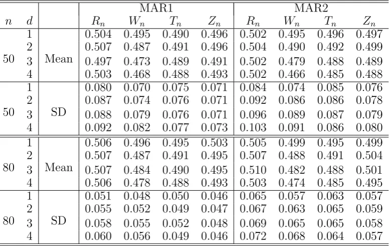
Table 1 reports the mean and standard deviation of the test statistics under H0 for the

the two sample t-test by obtaining inside information on the missedYs. Table 4 contains the empirical power for the setting where the outcomes were Gaussian and Gamma distributed respectively. We observe from Table 1 that there was a clear effect of the dimensionality on Wn with the mean deviating from 1/2 more and the variance increased as d was increased,

which was also the case for the variance of the propensity weighted test staitistic Rn. The

variance of Rn was consistently larger than that of Wn, Tn and Zn. This foreshadowed

a different test performance between the proposed and the propensity weighted tests. In contrast, the variance of the semiparametric Tn and Zn were not sensitive to d, indicating

the practical merits of the semiparametric extensions.

Table 2 indicates that all the tests considered had reasonable empirical size, which was especially the case for the two semiparametric tests. The slightly larger size distortion for the test based on Wn under d≥ 3 reflected the larger standard deviation in the mean from

1/2 as reported in Table 1. A deeper reason was the curse of dimension as Condition C3 was not met ford= 4 and just barely for d= 3, which was the motivation for proposing the semiparametric adjustments Tn and Zn. The performance of the semiparametric adjusted

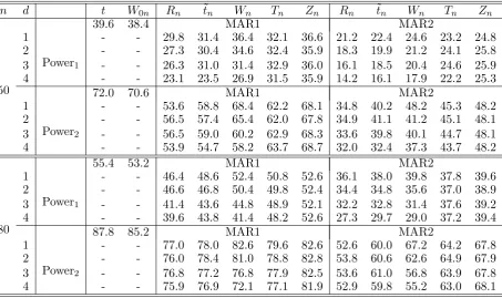
Mann-Whitney tests was very encouraging for both the size and power, and across different dimensions. We observe from Table 3 that the proposed nonparametric and semiparametric tests were much more powerful than the direct propensity adjusted Mann-Whitney test based onRnand the covariate adjustedt-test for almost all the Gaussian simulation settings

where the covariates and outcomes were all Gaussian, despite the settings were not that favorable to the proposed Mann-Whitney tests. Table 4 shows that, when the two outcome distributions were different, the powers of the proposed tests based on Wn, Tn and Zn

were much better than those of the tests based on Rn and ˜tn. As expected, both the

adjusted t-test and the impractical Oracle t-test broke down completely. Both Tables 3 and 4 show that the semiparametric test based on Zn (with the working linear function) was

consistently more powerful than that of the test based onTnusing propensity function. And

both semiparametric tests were consistently better than the tests based on Rn and ˜tn. Both

Tables 3 and 4 also reveal that the powers from proposed nonparametric and semiparametric tests were quite reasonable in comparison to the power of the Oracle Mann-Whitney test based on W0n.

7. A Data Analysis

(2008). Dehejia and Wahba (1999) considered propensity score match for comparison of two means, and Imbens (2004) conducted inverse probability weighting for the mean differ-ence. The datasets NSWRE74_CONTROL.TXT and NSWRE74_TREATED.TXT can be obtained at

http://www.nber.org/~rdehejia/nswdata.html. The dataset contains 445 individuals, 185 of whom participated in a training program and 260 did not. We are interested in the effect of the training program on earning in 1978. The covariates available for both groups (trained and not trained) include age, years of education, indicators of African-American and Hispanic-American, marital and degree statuses, and earnings in 1975. A comparison of the mean earnings of the two groups was considered in Qin et al. (2008). We consider here testing for the equality of the earning distributions. As advocated at the end of Section 2, in the formulation of the adjusted Mann-Whitney statistic Wn, we assignS = 1 for all the

185 individuals participated in the training program regarding them as “respondents” while assigningS = 0 for the rest of 260 individuals regarding them as “non-respondents” (missing outcomes). Similarly, in the second sample we treat the observations from 260 individuals not participated in the training program as “respondents” with S = 1 while regarding the other 185 individuals as “non-respondents” withS = 0.

Figure 1 displays the histograms of the earnings in 1978 for the trained and control groups, which conveys that both groups have a significant portion of members whose earnings were 0. The percentages of zero earnings were 35.4% and 24.3% in the control and trained groups respectively, which constitutes a quite sharp difference between the two groups. A direct application of the naive Mann-Whitney statistic, that ignored the pre-treatment covariates, on the earnings gave ap-value 0.011 and thus concluded a significant difference in the distri-butions of the earnings between the two groups. However, conditioning on earnings greater than zero, the distributions seem to be close to each other in Figure 1. This is confirmed by an application of the Mann-Whitney statistic on those with earnings greater zero, which gave ap-value of 0.374. In other words, the latter test could not reject the hypothesis that the distributions were the same for those with earnings greater than zero. However, both tests failed to reflect the observational nature of the data. In addition, we also observe from Figure 1 that the distributions of the earnings in 1978 are clearly not symmetric, indicating that t test may be less powerful in this case.

To gain more insights on the dataset and to reconcile the conflicting testing results mentioned above, we first apply the kernel estimator (2) to estimate the earning distributions F1 and F2 in 1978, adjusted with respect to covariate effect and missing values. The kernel

almost all quantiles of the trained group are consistently larger than those of the control group. Then we apply the proposed test statistics with adjustments to the covariate in comparing the earning distributions. We assume that individuals participated in the training program with a propensity function that depends on covariates. We use the product Gaussian kernel for smoothing the continuous covariates: the age, years of education and earnings in 1975. The bandwidths were chosen by the same approach as in the simulation study. The proposed bootstrap procedure was implemented to obtain the critical value of the test statistic with B = 100. The resulting test statistic Wn = 0.397, which was less than the

second smallest value, but greater than the smallest one, of the bootstrapped statistics. Hence thep-value was between 0.02 and 0.04 for a two sided test.

To apply the semiparametric test based on (13), we use the logistic model for the propen-sities of both groups. All covariates were included in the model with an additional quadratic term of age, which is suggested in Dehejia and Wahba (1999). Then we apply (13) to obtain Tn using the estimated propensity function. The bandwidth was chosen by cross-validation

and then divided by 2. The same bootstrap procedure was applied to calculate the critical value for Tn. The resulting test statistic Tn = 0.401 and the p-value was between 0.06 and

0.08. We then apply the working linear function approach using the same set of covariates as in the propensity function to getZn, and get the test statisticZn = 0.391 andp-value between

0.02 and 0.04. We find that the conclusions of the proposed tests are largely consistent with each other. Comparing the p-values of the proposed tests to that of the Mann-Whitney test that ignored the pre-treatment covariates, we observe substantial differences which clearly indicates the impact of the adjustment. This suggested that an adjustment to the covariate effect is important for analyzing data from observational studies.

Acknowledgements

We are very grateful to the Editor, AE, and two referees for their insightful comments and constructive suggestions that have greatly improved this paper. Chen acknowledges support from Center for Statistical Science at Peking University, and Tang acknowledges research support from National University of Singapore Academic research grants.

Appendix: Technical Details

A.1 Proof of Lemma 1

We start with an expansion for the Mann-Whitney statistic Wn which is used in proving

bandwidth used in ˆηm(x). We recall by its definition ηm(x) = πm(x)f(x). Applying Taylor’s

expansion, we have

1/ηˆm(x) = 1/ηm(x)−1/η2(x){ηˆm(x)−ηm(x)}+op(n

−_1/2

). (25)

Defineπmi=πm(Xmi),α1ik =π

−1

1i π

−1

2k,

α2ik =π

−₁

2k

{

n−₁

n

∑

j=1

Kh1(X1i−Xj)η

−₁

1 (Xj)−π

−₁

1i

}

,

α3ik =π

−₁

1i

{

n−₁

n

∑

l=1

Kh2(X2k−Xl)η

−₁

2 (Xl)−π

−₁

2k

}

,

α4ik =π_2k−1

{

n−1

n

∑

j=1

Kh1(X1i−Xj){ηˆ1(Xj)−η1(Xj)}η

−2

1 (Xj)

}

and

α5ik =π

−₁

1i

{

n−₁

n

∑

l=1

Kh2(X2k−Xl){ηˆ2(Xl)−η2(Xl)}η

−₂

2 (Xl)

}

.

Then, let Vik =I(Y1i ≤Y2k)S1iS2k, we have by substituting (25) into Wn defined by (4),

Wn =n

−₁ 1 n −₁ 2 n1 ∑ i=1 n2 ∑ k=1 Vik {

n−₁

n

∑

j=1

Kh1(X1i−Xj)ˆη

−₁

1 (Xj)

} {

n−₁

n

∑

l=1

Kh2(X2k−Xl)ˆη

−₁

2 (Xj)

}

=Wn1+Wn2+Wn3−Wn4−Wn5+op(n

−1/2

) (26)

where Wna = n

−₁

1 n

−₁

2

∑n1

i=1

∑n2

k=1Vikαaik for a = 1, . . . ,5. Here we note that the second

equation is just a re-organization of the terms as two-sample U- or V- statistics, and the op(n−1/2) term in (26) is from the approximation (25).

We note that Wn1 is a two-sample U-statistic, while Wn2, . . . , Wn5 are all related to

two-sample V-statistics (Serfling, 1980) after symmetrizing the summations. Let Omi =

(Xmi, Ymi, Smi) form = 1,2 and i= 1,· · · , nm, and define the projected statistic

˜

Wn1 =E(Wn1) + 2 ∑ m=1 nm ∑ j=1

{E(Wn1|Omj)−E(Wn1)}.

Then by applying the theory of U-statistics (Hoeffding, 1948; Serfling, 1980; Koroljuk and Borovskich, 1994),

Wn1−E(Wn1) ={W˜n1−E( ˜Wn1)}{1 +op(1)}. (27)

Clearly,E(Wn1) =

∫

F1(y)dF2(y) =θ, and it is straightforward to show that

˜

Wn1 =θ+n

−₁ 1 n1 ∑ i=1 { ¯

F2(Y1i)S1i

π1(X1i) −

θ }

+n−₁

2 n2 ∑

k=1

{

F1(Y2k)S2k

π2(X2k) −

θ }

where ¯F(y) is the survival function defined to be 1₋F(y).

As for Wn2, we define two kernels of two sample V-statistics by

h1(O1i, O1j;O2k) = 1/2{Vikπ

−₁

2kKh(X1i−X1j)η

−₁

1 (X1j) +Vjkπ

−₁

2kKh(X1j −X1i)η

−₁

1 (X1i)},

h2(O1i;O2k, O2j) = 1/2{Vikπ

−₁

2kKh(X1i−X2j)η

−₁

1 (X2j) +Vijπ

−₁

2j Kh(X1i−X2k)η

−₁

1 (X2k)},

Then the first part of Wn2 can be written as

W_n2(1) =n−₁

n−₁

1 n −₁ 2 { _n 1 ∑ i=1 n1 ∑ j=1 n2 ∑ k=1

h1(O1i, O1j;O2k) + n1 ∑ i=1 n2 ∑ j=1 n2 ∑ k=1

h1(O1i;O2j, O2k)

}

. (29)

By the V-statistics theory (Serfling, 1980), a V-statistic is equivalent in the first order to the U-statistic with the same kernel. Hence, by the projection method and note that

E_{h1(O1i, O1j;O2k)|O2k}=

F1(Y2k)S2k

π2(X2k)

, E_{h2(O1i;O2j, O2k)|O1i}=

¯

F2(Y1i)S1i

π1(X1i)

,

E_{h1(O1i, O1j;O2k)|O1i}= 1/2

{ ¯

F2(Y1i)S1i

π1(X1i)

+ ∫

¯

F2(y)dF1(y|X1i)

} and

E_{h2(O1i;O2j, O2k)|O2k}= 1/2

{

F1(Y2k)S2k

π2(X2k)

+ ∫

F1(y)dF2(y|X2k)

} .

Note that E(W_n2(1)) = θ and the projection of the second part of Wn2 is the same as (28).

Applying the same argument on Wn3, we obtain the following approximations to Wn2 and

Wn3,

˜

Wn2 =n

−₁

n

∑

j=1

{ξ1(Xj)−θ} and ˜Wn3 =n

−₁

n

∑

j=1

{ξ2(Xj)−θ}. (30)

Applying the same approach for the V-statistics in Wn4 and Wn5, we have the projected

statistics

˜

Wn4 =n

−₁ 1 n1 ∑ i=1 { S1i

π1(X1i)

ξ1(X1i)−θ

}

and ˜Wn5 =n

−₁ 2 n2 ∑ k=1 { S2k

π2(X2k)

ξ2(X2k)−θ

}

. (31)

Then Lemma 1 follows by combining (28), (30) and (31).

A.2 Proof of Lemma 2

For simplicity in presentation, we let β = (βT

1, β2T)T to be the combined unknown

pa-rameters in πm(x;β) for m = 1 and 2. Because {Xj}nj=1 = (X11, . . . , X1n1, X21, . . . , X2n2)

are independent and identically distributed (iid), _{t1j}nj=1 and {t2j}nj=1 are also iid. We note

that ˆtmj p

→tij as n→ ∞ and the approximation of ˆtmj is given by Taylor’s expansion

ˆ

tmj =πm(Xj; ˆβ) = πm(Xj, β0) +π

′

m(Xj; ˜β)( ˆβ−β0) = tmj +π

′

where ˜β _→p β0 as n → ∞. We now consider generic kernel smoothing taking the following

form with ˆtmj as smoother and Ω as a generic observable random variable:

ϕmi=n

−₁

m nm

∑

j=1

Khm(ˆtmi−ˆtmj)Ωj =n

−₁

m nm

∑

j=1

Khm(tmi−tmj+ ˆtmi−tmi−ˆtmj+tmj)Ωj.

=n−₁

m nm

∑

j=1

{

Khm(tmi−tmj) +K

′

ij(π

′

mi−π

′

mj)( ˆβ−β0)

} Ωj.

whereK′

ij =K

′

h{tmi−tmj+τij}withτij p

→0 andπ′

mi=π

′

(Xi; ˜β) as in (32). Clearly because

the smoothing is targeted at tmi, we have

n−1

m nm ∑ j=1 { K′

ij{π

′

mi−π

′

mj}( ˆβ−β0)

}

Ωj =f

′

(Xmi)(π

′

mi−π

′

mi)( ˆβ−β0)E(Ω|tmi){1 +op(1)}.

Because by the assumption C4 that ˆβ₋β0 is√n-consistent, we conclude

ϕmi=n

−₁

m nm

∑

j=1

Khm(tmi−tmj)Ωj+op(n

−_1/2

). (33)

In other words, using the estimated covariate as smoother brings in ignorable impact com-paring to using the corresponding true values. Then the remaining steps of proving Lemma 2 are exactly replicating those in proving Lemma 1 by replacing those Xmj byπm(Xmj, β0).

A.3 Proof of Lemma 3

The proof in A.2 already shows that smoothing at an estimated index value is first order equivalent to that at the truth. We now show that the impact due to estimating βm in the

propensity function is also negligible in ˆFm(y|z).

ˆ

fm(z) =n

−₁

m nm

∑

i=1

K(z₋Zmi)Smiπ

−₁

mi{1−π

−₁

mi(ˆπmi−πmi)}+op(n

−_1/2

)

=n−₁

nm

∑

i=1

K(z₋Zmi)Siπ

−₁

mi−fm(z)π

−₁

mi(ˆπmi−πmi) +op(n

−_1/2

)

Let ˆbm(y, z) = n−m1

∑nm

i=1I(Ymi ≤ y)K(z−Zmi)Smiπˆ

−₁

mi and denote its probability limit by

bm(y, z), it follows similarly that

ˆ

bm(y, z) =n

−₁

m nm

∑

i=1

I(Ymi≤y)K(z−Zmi)Smiπ

−₁

mi −bm(y, z)π

−₁

mi(ˆπmi−πmi) +op(n

−_1/2

).

Then substituting the above expressions into the following expansion,

ˆ

Fm(y|z) = ˆbm(y, z) ˆf

−₁

m (z) = ˆbm(y, z)f

−₁

m (z)[1−f

−₁

m (z){fˆm(z)−fm(z)}] +op(n

−_1/2

and note that the ˆπm terms exactly cancel each other. We note that this result is similar

to the finding in Wang et al. (1998). The rest proof of Lemma 3 is repeating the proof of Lemma 1 by replacing Xmi by gm(Xmi;γ0m).

A.4 Proof of Theorem 4

The same projection method as in proving Lemma 1 is applicable to derive the asymp-totic conditional distribution of W∗

n, with all the probability limits taken with respect to

the empirical distribution. In particular, √n_{W∗

n −E(W

∗

n|Fn)}/v∗ →d N(0,1) a.s. where

(v∗

)2 _{= lim}

n→∞nvar(W ∗

n|Fn). Let ˆλm(x) = n−1∑nj=1Khm(x − Xj)

ˆ η∗

m(Xj)−_ˆηm(Xj)

ˆ η2

m(Xj) ,ηˆ

∗

m(x) =

n−₁

m

∑nm

j=1Khm(x − X

∗

mj)S

∗

mj and ˆγm(x) = n−m1

∑nm

j=1

K_hm(x−_X∗ mj)

ˆ

ηm(Xmj∗ ) . By repeating the steps

in proving Lemma 1, we can establish an expansion of W∗

n resembling (26) given Fn as

W∗

n =W

∗

n1+W

∗

n2+W

∗

n3−W

∗

n4−W

∗

n5 +op(n−1/2) where for m= 1,2,

W∗

n1 =n

−₁ 1 n −₁ 2 n1 ∑ i=1 n2 ∑ k=1

I( ˜Y∗

1i ≤Y˜

∗

2k)S

∗

1iS

∗

2k

ˆ

π1(X1i∗)ˆπ2(X_2k∗ )

,πˆm(x) = ˆηm(x)/fˆm(x),

W∗

n2 =n

−1 1 n −1 2 n1 ∑ i=1 n2 ∑ k=1

I( ˜Y∗

1i ≤Y˜

∗

2k)S

∗

1iS

∗

2k

ˆ π2(X2k∗ )

{

n−1

n

∑

j=1

Kh1(X

∗

1i−X

∗

j)

ˆ η1(Xj∗)

−ˆγ1(X1i∗)

}

,

W∗

n4 =n

−₁ 1 n −₁ 2 n1 ∑ i=1 n2 ∑ k=1

I( ˜Y∗

1i ≤Y˜

∗

2k)S

∗

1iS

∗

2kλˆ1(X1i∗)

ˆ π2(X2k∗ )

,

and W∗

3n and W

∗

5n are respectively the second sample version of W

∗

2n and W

∗

4n by switching

indicesi and k other than those in the index function.

The crucial implication of the proposed bootstrap procedure is ˆG( ˜Y∗

mi) =Umi = ˆFm(Ymi∗ )

for m= 1,2. The joint distribution of each sample is respected in the following sense,

P( ˜Y∗

mi ≤y,X˜

∗

mi< x, S

∗

mi= 1) =P( ˆF

−₁

m {Gˆ( ˜Y

∗

mi)} ≤Fˆ

−₁

m {Gˆ(˜y)}, X

∗

mi< x, S

∗

mi= 1)

=P(Y∗

mi< ym, X

∗

mi< x, S

∗

mi = 1) for m= 1,2. (34)

Here ym and ˜y are connected such that ym is the ˆG(˜y)-th estimated quantile in the m-th

sample, for every ˜yin its sample space. It is clear that ˜Y∗

1i and ˜Y

∗

2i follow the same marginal

distribution ˆG. Under the null hypothesis the joint distribution is exactly preserved because

|ym−y˜|=|Fˆ

−₁

m {Gˆ(˜y)} −y˜| p

→ |F−₁

{F(˜y)_{} −}y˜_|= 0 as nm → ∞.

Then (34) implies as nm → ∞,P( ˜Ymi∗ ≤y, X˜

∗

mi< x, S

∗

mi= 1) p

→P(Ymi< y, Xmi < x, Smi=

1). Therefore, asn _{→ ∞},E(W∗

n|Fn) = 1/2 +o(n−1/2)a.s.It remains to show that under the

null hypothesis, lim

n→∞nvar(W ∗

n|Fn) → v2(1/2) a.s. This is because conditioning on Fn and

from (34), we have ω∗

2(x) =

∫ _ˆ

F1(˜y)dFˆ2(˜y|x) =

∫ _ˆ

G(˜y)dFˆ2(˜y|x) =

∫ _ˆ

F1(y1)dFˆ2(˜y|x). As n →

∞, under the null hypothesisym→y a.s.˜ form= 1,2, and henceω2∗(x)→

∫

F1(y)dF2(y|x) =

ξ2(x) a.s. Similarly

∫

{1₋Fˆ1(˜y)}dFˆ1(˜y|x) →ξ1(x) a.s. Theorem 3 then follows similarly as

References

Bilker, W. and Wang, M.-C. (1996), “A semiparametric extension of the Mann-Whitney test for randomly truncated data,” Biometrics, 52, 10–20.

Breslow, N. (2003), “Are statistical contributions to medicine undervalued?” Biometrics, 59, 1–8.

Cheng, P. E. (1994), “Nonparametric-estimation of mean functionals with data missing at random,” Journal of the American Statistical Association, 89, 81–87.

Cheung, Y. K. (2005), “Exact two-sample inference with missing data,” Biometrics, 61, 524–531.

Chu, C. K. and Chen, K. F. (1995), “Nonparametric regression estimates using misspecified binary responses,” Biometrika, 82, 315–325.

Dehejia, R. H. and Wahba, S. (1999), “Causal effects in nonexperimental studies: reevalua-tion the evaluareevalua-tion of training programs,” Journal of the American Statistical Association, 94, 1053–1062.

Fan, J. and Gijbels, I. (1996), Local Polynomial Modeling and Its Applications, Chapman and Hall, London.

Hahn, J. (1998), “On the role of the propensity score in efficient semiparametric estimation of average treatment effects,” Econometrica, 66, 315–331.

Hall, P., Racine, J., and Li, Q. (2004), “Cross-validation and the estimation of conditional probability densities,” Journal of the American Statistical Association, 99, 1015–1026.

Hall, P. and Yao, Q. (2005), “Approximating conditional distribution functions using dimen-sion reduction,” The Annals of Statistics, 33, 1404–1421.

Hansen, L. P. (1982), “Large sample properties of generalized method of moments estima-tors,” Econometrica, 50, 1029–1054.

H¨ardle, W. (1990), Applied Nonparametric Regression, Cambridge: Cambridge University Press.

Hirano, K., Imbens, G. W., and Ridder, G. (2003), “Efficient estimation of average treatment effects using the estimated propensity score,” Econometrica, 71, 1161–1189.

Hoeffding, W. (1948), “A class of statistics with asymptotically normal distribution,” The Annals of Mathematical Statistics, 19, 293–325.

Hu, Z., Follmann, D. A., and Qin, J. (2010), “Semiparametric dimension reduction estima-tion for mean response with missing data,” Biometrika, 97, 305–319.

— (2011), “Dimension reducted kernel estimation for distribution function with incomplete data,” Journal of Stat, 141, 3084–3093.

Imbens, G. (2004), “Nonparametric estimation of average treatment effects under exogeneity: a review,” Review of Economics and Statistics, 86, 4–30.

Korn, E. L. and Baumrind, S. (1998), “Clinician preferences and the estimation of causal treatment differences,” Statistical Science, 13, 209–235.

Koroljuk, V. S. and Borovskich, Y. V. (1994),Theory of U-Statistics, Kluwer, Dordrecht.

Kuk, A. Y. C. (1993), “A kernel method for estimating finite population functions using auxiliary information,” Biometrika, 80, 385–392.

Lalonde, R. J. (1986), “Evaluating the econometric evaluations of training programs with experimental data,” American Economic Review, 76, 604–620.

Little, R. and Rubin, D. (2002), Statistical Analysis With Missing Data, Wiley, 2nd ed.

Matloff, N. S. (1981), “Use of regression functions for improved estimation of means,”

Biometrika, 68, 685–689.

Newey, W. K. and McFadden, D. (1994), “Large sample estimation and hypothesis testing,”

Handbook of Econometrics, Vol 4, ed. by R. Engle and D. McFadden. New York: North Holland.

Qin, J., Shao, J., and Zhang, B. (2008), “Efficient and doubly robust imputation for covariate-dependent missing responses,” Journal of the American Statistical Association, 103, 797–810.

Rosenbaum, P. R. (2002), Observational Studies, Springer-Verlag: New York.

Rosenbaum, P. R. and Rubin, D. B. (1983), “The central role of the propensity score in observational studies for causal effects,” Biometrika, 70, 41–55.

Rubin, D. B. (1976), “Inference and missing values (with discussion),”Biometrika, 63, 581– 592.

Serfling, R. J. (1980), Approximation Theorems of Mathematical Statistics, John Wiley.

Tsiatis, A. A. (2006),Semiparametric Theory and Missing Data, Springer-Verlag: New York.

Table 1: Empirical means and standard deviations (SDs) ofRn,Wn,Tn (propensity function

based),Zn(working linear function based), given by (17), (4), (13) and (19) respectively, for

the Gaussian distributed responses under H0.

MAR1 MAR2

n d Rn Wn Tn Zn Rn Wn Tn Zn

1 0.504 0.495 0.490 0.496 0.502 0.495 0.496 0.497 2 0.507 0.487 0.491 0.496 0.504 0.490 0.492 0.499 50 _{3 Mean 0.497 0.473 0.489 0.491 0.502 0.479 0.488 0.489} 4 0.503 0.468 0.488 0.493 0.502 0.466 0.485 0.488 1 0.080 0.070 0.075 0.071 0.084 0.074 0.085 0.076 2 0.087 0.074 0.076 0.071 0.092 0.086 0.086 0.078 50 ₃ SD _{0.088 0.079 0.076 0.071 0.096 0.089 0.087 0.079} 4 0.092 0.082 0.077 0.073 0.103 0.091 0.086 0.080 1 0.506 0.496 0.495 0.503 0.505 0.499 0.495 0.499 2 0.507 0.487 0.491 0.495 0.507 0.488 0.491 0.504 80 _{3 Mean 0.507 0.484 0.490 0.495 0.510 0.482 0.488 0.501} 4 0.506 0.478 0.488 0.493 0.503 0.474 0.485 0.495 1 0.051 0.048 0.050 0.046 0.065 0.057 0.063 0.057 2 0.055 0.052 0.049 0.047 0.067 0.063 0.065 0.059 80 ₃ SD _{0.058 0.055 0.052 0.048 0.069 0.065 0.065 0.058} 4 0.060 0.056 0.049 0.046 0.072 0.068 0.064 0.057

Table 2: Empirical sizes (_×102_{) of the proposed nonparametrically and semiparametrically}

adjusted Mann-Whitney tests based onWn,Tn(propensity function) andZn (working linear

function), the tests based on the covariate adjusted Rn and ˜tn and the Oracle test W0n and

the two sample t test. The outcome distributions are Gaussian and α= 0.05.

n d t W0n Rn ˜tn Wn Tn Zn Rn ˜tn Wn Tn Zn

5.1 4.9 MAR1 MAR2

1 - - 5.1 4.7 5.2 5.4 4.8 5.8 5.5 5.4 5.2 5.2 2 - - 6.2 6.2 4.4 4.9 5.4 6.0 6.1 3.6 4.9 4.8 50 _{3 - - 5.7 6.0 4.1 4.5 5.4 6.3 6.5 3.3 5.2 5.3} 4 - - 5.9 6.2 3.5 5.4 5.2 6.7 6.9 3.0 4.6 4.5

4.8 5.3 MAR1 MAR2

Table 3: Empirical powers (_×102_{) of the proposed nonparametrically and semiparametrically}

adjusted Mann-Whitney tests based onWn,Tn(propensity function) andZn (working linear

function), the tests based on the covariate adjusted Rn and ˜tn and the Oracle test W0n and

the two sample t test. The outcome distributions are Gaussian and α= 0.05.

n d t W_0n R_n ˜t_n W_n T_n Z_n R_n t˜_n W_n T_n Z_n

39.6 38.4 MAR1 MAR2

1 - - 29.8 31.4 36.4 32.1 36.6 21.2 22.4 24.6 23.2 24.8

2 - - 27.3 30.4 34.6 32.4 35.9 18.3 19.9 21.2 24.1 25.8

3 Power1 - - 26.3 31.0 31.4 32.9 36.0 16.1 18.5 20.4 24.6 25.9

4 - - 23.1 23.5 26.9 31.5 35.9 14.2 16.1 17.9 22.2 25.3

50 _{72.0 70.6 MAR1 MAR2}

1 - - 53.6 58.8 68.4 62.2 68.1 34.8 40.2 48.2 45.3 48.2

2 - - 56.5 57.4 65.4 62.0 67.8 34.9 41.1 41.2 45.1 48.1

3 Power2 - - 56.5 59.0 60.2 62.9 68.3 33.6 39.8 40.1 44.7 48.1

4 - - 53.9 54.7 58.2 63.7 68.7 32.0 32.4 37.3 43.7 48.2

55.4 53.2 MAR1 MAR2

1 - - 46.4 48.6 52.4 50.8 52.6 36.1 38.0 39.8 37.8 39.6

2 - - 46.6 46.8 50.4 49.8 52.4 34.4 34.8 35.6 37.0 38.9

3 Power1 - - 41.4 43.6 44.8 48.9 52.1 32.2 32.8 31.4 37.6 39.2

4 - - 39.6 43.8 41.4 48.2 52.6 27.3 29.7 29.0 37.2 39.4

80 _{87.8 85.2 MAR1 MAR2}

1 - - 77.0 78.0 82.6 79.6 82.6 52.6 60.0 67.2 64.2 67.8

2 - - 76.0 78.4 81.0 78.8 82.8 53.8 60.6 62.6 64.9 67.9

3 Power2 - - 76.8 77.2 76.8 77.9 82.5 53.6 61.0 56.8 63.9 67.8

4 - - 75.9 76.9 72.1 77.1 81.9 52.9 59.8 55.2 63.0 68.1

Table 4: Empirical powers (_×102_{) the proposed nonparametrically and semiparametrically}

adjusted Mann-Whitney tests based onWn,Tn(propensity function) andZn (working linear

function), the tests based on the covariate adjusted Rn and ˜tn and the Oracle test W0n and

the two sample ttest. The outcome distributions are Gaussian and Gamma, and α= 0.05.

n d t W_0n R_n ˜t_n W_n T_n Z_n R_n ˜t_n W_n T_n Z_n

4.8 33.2 MAR1 MAR2

1 - - 19.4 8.8 27.8 23.6 28.1 16.4 4.6 22.1 17.7 23.6

2 - - 17.5 7.6 24.9 22.2 27.8 15.4 4.8 19.0 17.9 22.9

50 _{3 - - 15.3 5.1 20.9 24.1 27.9 14.7 6.3 16.7 17.7 23.3}

4 - - 13.6 3.0 17.8 23.8 27.7 13.1 3.9 15.9 17.5 23.2

5.3 42.6 MAR1 MAR2

1 - - 25.6 5.6 37.4 35.6 38.6 24.2 4.8 35.6 32.6 36.1

2 - - 24.4 4.4 37.0 35.9 39.1 21.4 4.2 33.4 33.6 36.2

80 _{3 - - 23.0 7.2 33.4 35.9 38.3 17.6 4.0 30.2 35.1 37.2}

Control Group

Earning in 1978

Frequency

0 10000 20000 30000 40000

0

20

40

60

80

100

120

Trained Group

Earning in 1978

Frequency

0 10000 20000 30000 40000 50000 60000

0

10

20

30

40

50

60

70

Figure 1: Histograms of the earnings in 1978

0 10000 20000 30000 40000

0.0

0.2

0.4

0.6

0.8

1.0

Estimated Distribution

Earning in 1978

CDF

Control Trained Pooled