Randomized Algorithm for Determining Stabilizing
Parameter Regions for General Delay Control Systems
*
Chao Yu, Binh-Nguyen Le, Xian Li, Qing-Guo Wang
Department of Electrical and Computer Engineering, National University of Singapore, Singapore City, Singapore. Email: [email protected], [email protected], [email protected], [email protected]
Received January 29th,2013; revised March 25th, 2013; accepted April 2nd, 2013
Copyright © 2013 Chao Yu et al. This is an open access article distributed under the Creative Commons Attribution License, which
permits unrestricted use, distribution, and reproduction in any medium, provided the original work is properly cited.
ABSTRACT
This paper proposes a method for determining the stabilizing parameter regions for general delay control systems based on randomized sampling. A delay control system is converted into a unified state-space form. The numerical stability condition is developed and checked for sample points in the parameter space. These points are separated into stable and unstable regions by the decision function obtained from some learning method. The proposed method is very general and applied to a much wider range of systems than the existing methods in the literature. The proposed method is illus-trated with examples.
Keywords: Stabilizing Parameter Regions; Delay Control Systems; Randomized Sampling; LMI Stability Criterion; Support Vector Machines
1. Introduction
Finding stabilizing regions for control systems in pa-rameter space becomes important in recent years. Stabi-lizing parameter regions will be instructive for controller tuning with greatest robustness or controller optimization with regard to other specific indexes. Most papers in the literature discuss about the stabilizing parameter re- gions for proportional-integral-derivative (PID) control-lers. Wang et al. [1] designed a quasi-Linear Matrix Ine-quality method to compute the stabilizing parameter re-gions of multi-loop PID controllers, but it only dealt with systems with no time delays. Lee et al. [2-4] established some stability conditions by simple P or PI controllers for a class of unstable processes with time delays, but the application of their methods is confined to single-input single-output (SISO) systems whose transfer functions only have one zero. Nie et al. [5] gave a frequency method to calculate the loop gain margins of multivari-able feedback system. Liu et al. [6] introduced a fast calculation approach for PI controller stable region based on D-partition method. Wang et al. [7] presented an
ef-fective graphical method to obtain exact P controller gain ranges for two input two output (TITO) systems with input time delay. However, this approach could not han-dle systems with state-delays. Some other methods can be found in [8-13]. All the methods seek the solutions for the stabilizing parameter regions for limited classes of plants or controllers.
In this paper, we design a general algorithm for deter-mining stabilizing parameter regions for delay control systems based on randomized sampling. Each unknown parameter is assumed to follow the uniform distribution in a given range and a certain number of independent and identically distributed (i.i.d.) random sample points are generated in the parameter space based on the random-ized algorithms [14]. Next, given a delay control system, we convert it into a unified state-space form. Efficient LMI stability criterion is developed for a control system with multiple delays in both input and state. Then each point in the parameter space is checked by the developed stability criterion. After that, these points are separated into stable and unstable regions by the decision function obtained from some learning method. The effectiveness of the proposed method is illustrated by simulation ex-amples.
*This research is funded by the Republic of Singapore’s National
Re-search Foundation through a grant to the Berkeley Education Alliance for Research in Singapore (BEARS) for the Singapore-Berkeley Build-ing Efficiency and Sustainability in the Tropics (SinBerBEST) Pro-gram. BEARS has been established by the University of California, Berkeley as a center for intellectual excellence in research and educa-tion in Singapore.
simulation examples and Section 6 concludes the paper.
2. The Proposed Method
[image:2.595.312.534.81.464.2]We consider a unity feedback control system as shown in Figure 1. The plant may have some unknown parameters that may affect the system stability and the parameters of the controller are also needed to be designed. Hence, knowing stabilizing parameter regions is instructive for robustness analysis and design. Some methods [2-4] can give analytical solutions for stabilizing parameter regions, but these methods usually have many constraints and could only be applied to limited plants or controllers. Some numerical methods [11,12] also have some restric-tions on system structures and their algorithms might be difficult to be implemented. The objective of this paper is to provide stabilizing parameter regions with a new ap-proach which is totally different from the existing meth-ods in this specific area. We illustrate the idea of our method with a simple example.
We consider the model in [10] as follows,
5 4 3 32 24 1
,
2 32 14 4 50
s s s
G s
s s s s s
with a PI controller
i,p
K C s K
s
where Kp and Ki are unknown parameters. With the
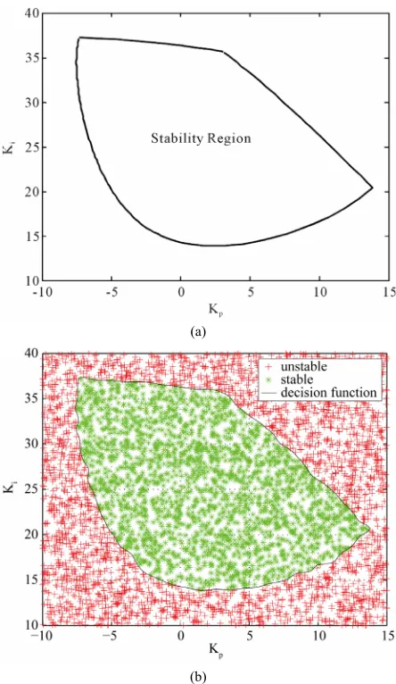
method in [10], the stabilizing parameter region is shown in Figure 2(a).
The randomized algorithms have been applied to de-sign robust controllers [14]. In their context, a fixed sin-gle controller is obtained for an uncertain plant. The un-certainty lies in some plant parameters. These parameters are sampled randomly to get a set of plants which repre-sent and replace the original uncertain plant. One single controller (fixed controller parameters) is found to meet a performance measure such as H for these sampled points. In our context, we want to find the entire regions of controller parameters which stabilize a plant. Fur-thermore, the plant may also have some uncertain pa-rameters such as delay. In the later case, we want to find the regions of combined parameter vector p from the controller and the plant which stabilize the control sys-tem. We employ the idea of randomized sampling. Sup-pose that each unknown parameter follows the uniform distribution in a given range, that is Kp
10,15
,
10, 40
i
[image:2.595.56.253.328.394.2]K and they distribute uniformly in their re-
Figure 1. Unity feedback control system.
(a)
(b)
Figure 2. Stabilizing parameter region for the example in [10]. (a) Result in [10]; (b) Result with the proposed method.
spective range. Then a certain number of i.i.d. random points are sampled in the parameter space. Repeated samples are omitted. According to the randomized algo-rithms [14], the number of points, N, should satisfy
2
1 ln ,2 2 N
(1) where we set a priori
0,1 as the accuracy parame- ter and
0,1 as the confidence level. Both and are usually taken small values, say less than 0.1. We choose 0.02 and 0.05 for our example. It could be calculated from (1) that N4611 and then we choose
5000
N . Throughout this paper, is used for all simulation cases.
5000
N
Next, we check whether each of these points could stabilize the system by some stability criterion. The cha- racteristic equation of the closed-loop system is
6 5 4 3
2
2 3 4 14
4 4 50 0.
p p i
i p p i i
s s K s K K s
K K s K K s K
[image:2.595.58.286.667.722.2]We can simply calculate the closed-loop poles for sta-bility testing. If a point of Kp,Ki could stabilize the
system, it is labeled as “stable”. Otherwise, if a point could not stabilize the system, it is labeled as “unstable”. However, calculating the closed-loop poles is not possi-ble for systems with time delays. In this case, we present a Linear Matrix Inequality (LMI) stability criterion which will be discussed in next section.
Lastly, the points in the parameter space are divided into stable and unstable regions by the decision function obtained from some learning method, such as the Neural Networks and the Support Vector Machines (SVM) [15]. We choose SVM as the classification tool and employ the LibSVM [16] kit with its arguments “-t” = 2 (Radial Basis Function (RBF) as kernel) and “-c” = 1,000,000 (penalty parameter) to solve the problem. The resulting stabilizing parameter region is shown in Figure 2(b). It is seen from Figures 2(a) and (b) that the stable region from the proposed method is almost same as that in [10]. Hence, our method is effective and straightforward.
3. Stability Criterion
As stated in previous section, it is impossible to calculate the closed-loop poles for systems with time delays. Therefore, in this section, we present an effective algo-rithm for stability testing which can be applied to a much wider range of systems. Given a delay system with PI or PID controller, we first convert it into a unified state- space form, which is a generalization of the method in [17] where a delay-free system is considered. Next, we present a conversion of delay systems with general dy-namic controllers. Lastly, we present an LMI stability criterion for the unified state-space form.
3.1. PI Control for Input-Delay Plant
Consider a plant:
, ,
x t Ax t Bu t d y t Cx t
(2) with a PI controller:
1
2
0d .
t
u t F y t F
y Let
1
20
, d
t
x t z t
z t
z t y t
so that
1
20
. d
t d
x t d z t d
z t d
z t d y
The vector z t
can be viewed as a new state vari-able of the system, whose dynamics is governed by
0
,0 0
A B
z t z t u t d
C
(3)
where
1 1 2 2
1 1
1 2
2 2
0 0
u t F Cz t F z t
z t z t
F C F I
z t z t
.
(4)
Let C1
C 0
and C2
0 I
. Equation (4) can be rewritten as
1 1 2 2
, u t F C F C z tor
1 1 2 2
.u td F C F C z td
(5) Substituting (5) into (3) yields
1
,z t Az t A z t d
(6) where0 , 0 A A
C
and
1 0 1 1 2 .
B
2 A F C F C
When (2) is with a PID controller
1
2
3
0d d
d
t
y t
u t F y t F y F
t
,the conversion could not be proceeded. This is because
u t depends on u t
d
since
dy t
dt CAx t CBu t d
. Then the control signal cannot be expressed only by state vectors as (4) or (5). In such a case, we could use a practical D controller:
, 1
d s
s N
where d is chosen by users to limit derivative gain on
higher frequencies. Then, the practical PID controller falls in a format of general dynamic controller, which is handled in Section 3.3 below.
N
3.2. PID Control for State-Delay Plant
Consider a plant:
1, ,
x t Ax t A x t d Bu t y t Cx t
with a PID controller:
1
2
3
0 d d . d t y tu t F y t F y F
t
Let z t1
x t
and 2
0d
t
z t
y . We have
1 1 1 1 ,
z t x t Az t A z td Bu t and
2 1 .
z t y t Cz t Denoting
T
T T, we have1 , 2 z t z t z t
1
, z t Az t A z td Bu t where1 1
0 0
, ,
0 0 0 0 .
A A B
A A B
C , Combining (7) and the definition of z yields
1
12 0 z t , y t Cz t C
z t
1
22 0
d 0
t z t
y z t I
z t
and
1 1 d d, 0 ,0 .
y t
Cx t CAx t CA x t d CBu t t
CA z t CA z t d CBu t
Denoting C1
C 0
, C2
0 I
, C3
CA 0
,
1 0
d
C CA , y t1
C z t1
, y2
t C z t2
and
3 3 d
y t C z t C z td , we have
1 1
2 2
3 3
3
. u t F y t F y t F y t F CBu t Suppose that
IF CB3
is invertible. Let
T
T
T
T 1 , 2 , 3y t y t y t y t , C C1T,C2T,C3TT, T
T 0, 0,
d d
C C , and F F F F1, ,2 3, where
1 1 3 1 2 3 1 3 3 , , . 1 2 3 F I F CB F F I F CB F F I F CB F
Then (7) is equivalent to
1 ,
, d
z t Az t A z t d Bu t y t Cz t C z t d
with
, u t Fy t i.e.,
1 1 , d dz t Az t A z t d BFCz t BFC z t d
A BFC z t A BFC z t d
(8)
which is also in the form of (6) with A
ABFC
and A1
A1BFCd
.Remark 1. The systems (2) and (7) only contain one time delay. However, it would not be difficult to make conversion for systems with multiple time delays, which is omitted here for brevity.
The previous two cases only tackle delay systems with PI or PID controller whose parameters appear in a linear form. In practical control systems, the controllers may be of higher orders and the parameters of controllers may also appear in a nonlinear form, such as the lead-lag compensators [18]. Thus, we consider the conversion for delay systems with general dynamic controller as fol-lows.
3.3. General Dynamic Controller for a Plant with Multiple Delays in Input and State
Consider a plant (9)
1 1 2 2
1
2 2 ,
.
h h h
h l h l
x t Ax t A x t d A x t d
A x t d Bu t B u t d
B u t d B u t d
y t Cx t
1 (9)
under the following dynamic controller:
0 1 1 11 1 1 , m m m m n n n n
b s b s b s b
C s
s a s a s a
whose minimal state-space realization can be expressed by
, . c c c cv t A v t B y t
u t C v t D y t
Let z t1
x t
T T
and z2
t v t . Denoting
T1 , 2
z t z t z t , we have
1
2
, z t x t z t
z t v t
and
1
2.
i i
i
i i
z t d x t d
z t d
z t d v t d
1 h
1 1 1 1 1 1
1 2 1 1
1 2 1 1
2 .
h h
c c c
c h l c h l l c h l
z t Az t A z t d A z t d
BD Cz t BC z t B D Cz t d
B C z t d B D Cz t d
B C z t d
(10)
and
2 c 1 c 2 ,
z t B Cz t A z t i.e.,
1 , k i iz t Az t A z t d
i
,
(11)
0
, for 0
0 0
, for ,
0 0
i
i
i h c i h c A
i h A
B D C B C
h i k
and k h l.
Remark 2. The system (6) is a special case of (11). 3.4. The LMI Stability Criterion for a System
with Multiple Delays in Input and State
Theorem 1. The system (11) is asymptotically stable if there exist symmetric positive definite matrices ,
, and , such that
1 , , P Q
k
Q W1, ,Wk where 0,
(12)
,
c c
c c
A BD C BC A
B C A
where (13) holds,
T
1 1 2 2
=1 =1 1 1 2 2 0 0 . 0 k k
i i k k
i i
k k
A P PA Q W PA W PA W PA W
Q W Q W Q W
k (13) T T 1 1 T T1 1 1 1
T T
1 1
,
k k k k
k k k
d A W d A W
d A W d A W
d A W d A W
and 1 2 0 0 . 0 k W W W
Here and in the sequel, a block induced by symmetry is denoted by an ellipsis *. Proof. Define the Lyapunov functional as
T
T
0 T
=1 =1
d d
i i
t t
k k
i i i
i t d i d t
V z t z t Pz t z s Q z s s d z s W z s s
d .
i iThe derivative of V z t
is
T T T T
=1 =1
2 T T
=1 =1
d .
i
k k
i i i
i i
t
k k
i i i i
i i t d
V z t z t Pz t z t Pz t z t Q z t z t d Q z t d
d z t W z t d z sW z s s
It follows from Jensen’s inequality [19] that
T
T d .
i
t
i i i i
t d
d z s W z s s z t z t d W z t z t d
T T
=1 =1
T T
=1 =1
T 2
=1 =1 =1
T =1
.
k k
i i i i
i i
k k
i i i i
i i
k k k
i i i i i i
i i i
k
i i i
i
V z t z t P Az t A z t d Az t A z t d Pz t
z t Q z t z t d Q z t d
d Az t A z t d W Az t A z t d
z t z t d W z t z t d
(14)
Let
T
T
T
T1 k ,
w t z t z td z td
and
1 k .
A A A
One sees
T
2 T
=1
.
k
i i i
V z t w t d W w t
By Schur complement, (12) guarantees
2 T
=1
0.
k
i i i
d W
Therefore, the system (11) is asymptotically stable.
4. Stabilizing Parameter Regions
Each point in the parameter space corresponds to a sam-ple of the parameter vector p, which is denoted by i,
. We check whether each of these points could stabilize the system by the developed LMI stability crite-rion. If a point i could stabilize the system, it is
la-beled as “stable”. Otherwise, if i could not stabilize
the system, it is labeled as “unstable”.
p 1, ,
i N
p
p
The points in the parameter space can be separated into stable and unstable regions by the decision function obtained from some learning method. In this paper, we choose SVM as the learning method due to its superior performance in a wide range of applications. Support Vector Machines (SVM), which was first introduced by Vapnik [20], has shown many attractive features in the fields of small sample, non-linear and high dimensional pattern recognition [21]. It can be promoted to classifica-tion and regression problems. It employs the Structural Risk Minimization principle [21]. The goal of SVM is to find a decision function that minimizes the structural risk, which could be converted into a quadratic programming problem. In addition, the solution of an SVM problem is a globally optimal solution [22].
In this paper, SVM is employed to solve a binary classification problem. Given the data set
S S1, , ,2 SN
S
p
with , where
i is a point in the parameter space and (stable)
or −1 (unstable) is the label of the point, SVM is to solve the following problem:
,
, 1, 2, ,i i i
S p y i 1
i
y N
T
1 1 1
1
1
max ,
2
subject to 0, 0 ,
N N N
i i j i j i
i i j
N
i i i
i
j
y y p p
y C
where is the Lagrange multiplier, is the penalty parameter which can be set by users and
0 C
is a mapping from i to a higher dimensional space.
There have already been many SVM tool kits that can be used to solve the classification problems. LIBSVM [16] is a simple and effective one developed by Chih-Jen Lin’s research group. Throughout this paper, the LibSVM kit is employed to do simulation with proper arguments.
p
5. Simulation Examples
In this section, four examples are presented to illustrate the effectiveness of the proposed method.
Example 1. The analytical method in [2] cannot deal with a process containing multiple zeros, while our method does not have this constraint. Consider the plant:
0.4
1 0.2
1
e , 1 0.5 1 0.1 1ds
s s
G s
s s s
with a P controller C s
kI2. This control system is converted to the form in (11) with1
11 8 20
1 0 0 ,
0 1 0
1.6 12 20
0 0 0
0 0 0
A
k k k
A
.
Figure 3. Stabilizing parameter region for Example 1.
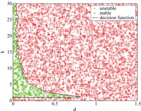
Example 2. The graphical method in [7] cannot deal with a process containing state-delays. However, our method does not have this restriction. Consider the plant:
12.5 251 0
0 10 1
,
1.5 0 0
0 25 ,
x t x t
x t d u t
y t x t
(15)
with a P controller . This control system is converted to the form in (11) with
u ky
1
12.5 25 25 ,
1 0
0 10 . 1.5 0
k A
A
Let p
d k, . Performing our method with “-t” = 2 and “-c” = 1000, the stabilizing parameter region is obtained and shown in Figure 4.Example 3. Consider the plant (15) with d 0.5 under the controller
a . C ss b
(16)
Note that b appears in a nonlinear fashion, which is different from parameters of PID controllers. We can rewrite (16) as
, . v t bv t y t u t av t
This control system is converted to the form in (11) with
Figure 4. Stabilizing parameter region for Example 2.
1
12.5 25 0 10 0
1 0 0 , 1.5 0 0
0 25 0 0 0
a
A A
b
.
Let p
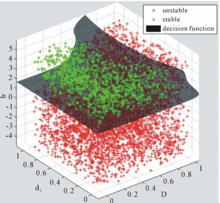
b a, . Performing our method with “-t” = 2 and “-c” = 1000, the stabilizing parameter region is ob-tained and shown in Figure 5.Example 4. The proposed method also works well with a high-dimensional parameter space. Consider the plant:
1 2
12.5 25
1 0
0 10 1
,
1.5 0 0
0 25 ,
x t x t
x t d u t dy t x t
with a controller:
, .
v t bv t y t u t v t
0
This control system is converted to the form in (11) with
1
2
12.5 25 0 0 10 0
1 0 0 , 1.5 0
0 25 0 0 0
0 0 1
and 0 0 0 .
0 0 0
A A
b
A
Let p
d d b1, ,2
. Performing our method with “-t” = [image:7.595.311.538.86.264.2]Figure 5. Stabilizing parameter region for Example 3.
Figure 6. Stabilizing parameter region for Example 4.
The above examples have well illustrated the effec-tiveness of the proposed method which can be applied to a much wider range of systems than the existing methods in the literature.
6. Conclusions
This paper proposes a new and general method for de-termining the stabilizing parameter regions for delay control systems. We first take a certain number of ran-dom sample points in the parameter space. Next, we rep-resent a delay control system in a unified state-space form. Then the numerical stability condition is developed and checked for sample points in the parameter space. These points are divided into two classes according to whether they can stabilize the system. The stabilizing parameter regions could be well defined by the decision
function obtained from some learning method. The effec-tiveness of the proposed method is well illustrated with examples. The proposed method does not have essential constraints and has a wide range of applications. Note that our method could be applied to a higher-dimensional parameter space, though the stabilizing parameter regions are difficult to be shown by graphics.
It should be pointed out that the presented LMI stabil-ity criterion is only sufficient since it is based on Lya- punov theory. A sufficient and necessary stability crite- rion and the additional potential values of the proposed method are to be investigated in future works.
REFERENCES
[1] Q. Wang, C. Lin, Z. Ye, G. Wen, Y. He and C. Hang, “A Quasilmi Approach to Computing Stabilizing Parameter Ranges of Multi-Loop Pid Controllers,” Journal of Proc- ess Control, Vol. 17, No. 1, 2007, pp. 59-72.
doi:10.1016/j.jprocont.2006.08.006
[2] S. Lee and Q. Wang, “Stabilization Conditions for a Class of Unstable Delay Processes of Higher Order,” Journal of the Taiwan Institute of Chemical Engineers, Vol. 41, No.
4, 2010, pp. 440-445. doi:10.1016/j.jtice.2010.03.001
[3] S. Lee, Q. Wang and C. Xiang, “Stabilization of All-Pole Unstable Delay Processes by Simple Controllers,” Jour- nal ofProcess Control, Vol. 20, No. 2, 2010, pp. 235-239.
doi:10.1016/j.jprocont.2009.05.005
[4] S. Lee, Q. Wang and L. Nguyen, “Stabilizing Control for a Class of Delay Unstable Processes,” ISA transactions, Vol. 49, No. 3, 2010, pp. 318-325.
doi:10.1016/j.isatra.2010.03.006
[5] Z. Nie, Q. Wang, M. Wu and Y. He, “Exact Computation of Loop Gain Margins of Multivariable Feedback Sys- tems,” Journal of Process Control, Vol. 20, No. 6, 2010,
pp. 762-768. doi:10.1016/j.jprocont.2010.04.006
[6] L. Jinggong, X. Yali and L. Donghai, “Calculation of Pi Controller Stable Region Based on d-Partition Method,” 2010 International Conference on Control Automation and Systems (ICCAS), Gyeonggi-do, 27-30 October 2010, pp.
2185-2189.
[7] Q. Wang, B. Le and T. Lee, “Graphical Methods for Computation of Stabilizing Gain Ranges for Tito Sys- tems,” 2011 9th IEEE International Conference on Con- trol and Automation (ICCA), Santiago, 19-21 December 2011, pp. 82-87.
[8] Q. Wang, Y. He, Z. Ye, C. Lin and C. Hang, “On Loop Phase Margins of Multivariable Control Systems,” Jour- nal of Process Control, Vol. 18, No. 2, 2008, pp. 202-211.
doi:10.1016/j.jprocont.2007.06.004
[9] M. S¨oylemez, N. Munro and H. Baki, “Fast Calculation of Stabilizing Pid Controllers,” Automatica, Vol. 39, No.
1, 2003, pp. 121-126.
doi:10.1016/S0005-1098(02)00180-2
[image:8.595.60.287.297.507.2]agement, Vol. 47, No. 18, 2006, pp. 3045-3058.
doi:10.1016/j.enconman.2006.03.022
[11] B. Fang, “Computation of Stabilizing Pid Gain Regions Based on the Inverse Nyquist Plot,” Journal of Process Control, Vol. 20, No. 10, 2010, pp. 1183-1187.
doi:10.1016/j.jprocont.2010.07.004
[12] E. Gryazina and B. Polyak, “Stability Regions in the Pa- rameter Space: D-Decomposition Revisited,” Automatica,
Vol. 42, No. 1, 2006, pp. 13-26.
doi:10.1016/j.automatica.2005.08.010
[13] K. Saadaoui, S. Testouri and M. Benrejeb, “Robust Stabi- lizing First-Order Controllers for a Class of Time Delay Systems,” ISA transactions, Vol. 49, No. 3, 2010, pp. 277-
282. doi:10.1016/j.isatra.2010.02.001
[14] G. Calafiore, F. Dabbene and R. Tempo, “Research on Probabilistic Methods for Control System Design,” Auto- matica, Vol. 47, No. 7, 2011, pp. 1279-1293.
doi:10.1016/j.automatica.2011.02.029
[15] T. Hastie, R. Tibshirani and J. H. Friedman, “The Ele- ments of Statistical Learning: Data Mining, Inference, and Prediction,” Springer, New York, 2009.
doi:10.1007/978-0-387-84858-7
[16] C. C. Chang and C. J. Lin, “LIBSVM: A Library for Sup- port Vector Machines,” ACM Transactions on Intelligent Systems and Technology (TIST), Vol. 2, No. 3, 2011, p.
27. doi:10.1145/1961189.1961199
[17] F. Zheng, Q. Wang and T. Lee, “On the Design of Multi- variable PID Controllers via LMI Approach,” Automatica,
Vol. 38, No. 3, 2002, pp. 517-526.
doi:10.1016/S0005-1098(01)00237-0
[18] G. Franklin, J. Powell, A. Emami-Naeini and J. Powell, “Feedback Control of Dynamic Systems,” , Vol. 3, Addi- son-Wesley, Reading, 1994.
[19] K. Gu, V. Kharitonov and J. Chen, “Stability of Time- Delay Systems,” Birkhauser, Boston, 2003.
doi:10.1007/978-1-4612-0039-0
[20] V. Vapnik, “The Nature of Statistical Learning Theory,” 1995.
[21] S. R. Gunn, “Support Vector Machines for Classification and Regression,” ISIS Technical Report, Vol. 14, 1998.
[22] P. H. Chen, C. J. Lin and B. Schölkopf, “A Tutorial on ν- Support Vector Machines,” Applied Stochastic Models in Business and Industry, Vol. 21, No. 2, 2005, pp. 111-