On a New Equation for Critical Current Density Directly
in Terms of the BCS Interaction Parameter, Debye
Temperature and the Fermi Energy of the Superconductor
G. P. Malik*
Theory Group, School of Environmental Sciences, Jawaharlal Nehru University, New Delhi, India. Email: [email protected], [email protected]
Received February 7th, 2013; revised March 11th, 2013; accepted March 29th, 2013
Copyright © 2013 G.P. Malik. This is an open access article distributed under the Creative Commons Attribution License, which permits unrestricted use, distribution, and reproduction in any medium, provided the original work is properly cited.
ABSTRACT
Recasting the BCS theory in the larger framework of the Bethe-Salpeter equation, a new equation is derived for the temperature-dependent critical current density jc(T) of an elemental superconductor (SC) directly in terms of the basic parameters of the theory, namely the dimensionless coupling constant [N(0)V], the Debye temperature θD and, addi-tionally, the Fermi energy EF—unlike earlier such equations based on diverse, indirect criteria. Our approach provides an ab initio theoretical justification for one of the latter, text book equations invoked at T = 0 which involves Fermi momentum; additionally, it relates jc with the relevant parameters of the problem at T≠ 0. Noting that the numerical value of EF of a high-Tc SC is a necessary input for the construction of its Fermi surface—which sheds light on its gap-structure, we also briefly discuss extension of our approach for such SCs.
Keywords: Critical Current Density; BCS Parameters; Fermi Energy; Elemental/Non-Elemental Superconductors
1. Introduction
The critical current density (jc) of a superconductor (SC) is the maximum current density that it can carry beyond which it loses the characteristic of superconductivity. It is an important parameter because greater its value, greater is the practical use to which the SC can be put. The basic
relation between jc and the critical velocity (vc) of Cooper pairs (CPs) at any temperature T and an applied field H is:
,
,
*
,
,
2
c s c c c
j T H n T H e v T H v P m* (1)
where ns is the number of CPs, e*, Pc and (2m*) are, re- spectively, the charge, the critical momentum, and the effective mass of a CP. We note that, since formation of CPs in the BCS theory is synonymous with the formation of their condensate [e.g., 1], Pc in (1) may also be defined as the minimum momentum that causes dissociation of the condensate.
As alternatives to (1), several derived relations for jc can be found in the literature [2-5], some of which have been reproduced in Table 1. Salient features of these
relations are: 1) They are obtained via indirect approaches based on diverse criteria such as the type of SC being dealt
with (type I or II) and its geometry; 2) They lead to values of jcs that are generally much greater than the experi- mental values; and 3) Only one of them involves the Fer- mi energy EF (via Fermi momentum) of the SC—this will be further discussed below.
EF of an SC is an important parameter too because, as has been remarked [6], “There is every evidence that the remarkable low value of EF (<100 meV) and the strong coupling of carriers with high-frequency phonons is the cause of high Tc in all newly discovered superconduc- tors.” Furthermore, the input of the numerical value of EF is essential to construct the Fermi surface Ej(k) of an SC via j
F, from which it is seen that [7; p. 117] the whole process of determining theoretically the shapeE k E
of the Fermi surface involves calculating Ej(k) over the entire Brillouin zone and then constructing the particular constant energy surface that corresponds to EF. However, this assumes that the actual numerical value of EF is available, which may well not be the case. The impor- tance of the Fermi surface stems from the fact it sheds light on the gap-structure of the SC since it marks the boundary between the occupied and the unoccupied parts of the band j. This explains the considerable experimen- tal effort that has been expended on constructing the
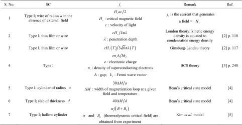
Table 1. Some of the relations in the literature for calculating the critical current densities (jcs) of different types of super-conductors obtained via diverse, indirect methods.
S. No. SC jc Remark Ref.
1 Type I; wire of radius absence of external field a in the
2 c H ac
c
H : critical magnetic field c: velocity of light
c
j is the current that generates a field = Hc
2 Type I; thin film or wire cHc 4π
: penetration depth
London theory; kinetic energy density is equated to condensation energy density
[2] p. 118
3 Type I; thin film or wire cH Tc 3 6π T Ginsburg-Landau theory [2] p. 117
4 Type I
s F
en k
e: electronic charge
s
n : density of superconducting electrons
: gap; kF: Fermi wave vector
BCS theory [3] p. 248
5 Type I; cylinder of radius a
30M a M
: width of magnetization loop at a given field and temperature
Bean’s critical state model [4]
6 Type I; slab of thickness d 40M d Bean’s critical state model [4]
7 Type I; hollow cylinder
B B0
and B0 (thermodynamic critical field) are
obtained from experiment
Kim et al. model [5]
Fermi surfaces of a variety of high-Tc SCs as reported in [e.g., 8,9] and, more recently, in [10-12]. In particular, in the latter of these references, the gaps observed in iron- pnictide SCs as nodes or line nodes on the Fermi surface have evinced considerable interest. For a quantitative account of the Tc and the multiple gaps of a prominent member of the iron-pnictide family, namely
Ba0.6K0.4Fe2As2, in the framework of the generalized- BCS equations (GBCSEs) [13]—which will be further discussed below, we draw attention to [14].
The purpose of this note is to present an approach in which Pc(T)—defined as the momentum at which the binding energy of the CPs vanishes (this is equivalent to the vanishing of the gap [13])—is calculated via the dy- namics of CPs. As will be seen, we are then led via (1) to an equation for jc(T) directly in terms of the familiar BCS parameters, namely the dimensionless coupling constant [N(0)V], the Debye temperature θD and, additionally, EF of the SC. The framework employed by us is that of the Bethe-Salpeter equation (BSE) for reasons to be spelled out shortly.
The paper is organized as follows. In the next section, we obtain equations for Pc(T, H = 0) and Pc(T = 0, H = 0) for a simple SC. The solutions of these equations for Sn are obtained in Section 3 and compared with similar re- sults obtained by a different method. Extension of our approach for non-elemental SCs is presented in Section 4. In Section 5 we make four brief comments. The final section sums up our conclusions.
2. Equations for
P
c(
T
,
H
= 0) and
P
c(
T
= 0,
H
= 0) for a Simple SC
Our starting point is the T = 0, H = 0 BSE [15] for the bound states of particles a, b bound via the interaction kernel ,
c a b
I in the ladder and instantaneous approxima- tions:
1 4
,2π d c q
a b a b
F F p i q p q I
. (2)Customization of this equation for CPs requires th at a, b should be electrons. We then have
1 1
1 2
1 2
a a
a
b b
b ,
F P p m i
F P p m i
(3) where m is the electron mass, a b,
are the Dirac matrices,
p
are 4-momenta of the two electrons in the centre of mass (c.m.) frame, and P is the 4-momentum of the c.m.
of the CP in the laboratory frame.
In our earlier work [13] based on (2), it sufficed to set
, 0 ;
= 2 F
P E E E W (4) where E is the total energy of a CP; it then turned out that
W . The BCS interaction kernel in (2) then was
, 3
2 2
0 for 2π
,
2 2
q p
p q
c a b
F D F D
V
I V
E E
m m
[Note: We use natural units: mass, momentum, energy, etc. in eV, c 1].
The role of the 4th dimension in (2) is simply to pro- vide the means to temperature-generalize the theory at the outset via the Matsubara recipe. Thus, following the steps that have been detailed in [13,16] we obtain from (2) the 3-dimensional equation
1 3
,
2π d
p c q p
a b
S i
qI S q J q , (6) where
4 4 2 4 4 ,2 2 ,
,
,
p p p
p p
p p
q p q p
c a b c
ab ab
S p A B p p
A E m
B A I I (7) and
4
4 4 d q q q q J
q A B q
(8)If we simply carry out the integration in (8), we obtain the usual T = 0 theory; subjecting it to the Matsubara recipe, however, we obtain an equation valid at any tem- perature—causing the theory to incorporate many-body effects. With the aid of the Matsubara recipe, (8) yields [13,16]:
tan h
2
tan h
2
π A q B q
J q i
D q
, (9)
where
q
q
q
q2D A B E m
, (9) and 1 k TB , kB being the Boltzmann constant.Since critical velocity is defined as the velocity of CPs at which W = 0, we now need to consider (2) for the case of moving CPs. Hence (4) is replaced by
,pP E
(11)where is the 3-momentum of the c.m. of a CP. It i s pertinent at this stage to draw attention to the intera ction Hamiltonian corresponding to (2), which is actua lly apparent from the structure of the equation:
p
int,BSE
H g
where ψ is the electron field and the phonon field; exchanges of the latter field between the electrons with coupling strength g being responsible for pairing. Both for elemental and non-elemental SCs, one is now enabled to calculate not only the Tcs and ∆s—as has been shown [17,18], but also Pc(T)s of the pairs as will be seen below.
Because the BSE formalism accommodates CPs having
non-zero c.m. momentum, it constitutes a larger frame- work than the original BCS formalism which restricts the Hamiltonian at the outset to comprise of terms corre- sponding to pairs having zero c.m. momentum.
Since energies of the electrons forming a CP now take on the values
P 2porq
2 2m, the BCS model interaction given in (5) gets replaced by
3 2 20 for 2π
2 or 2 or
,
2 2
0 otherwise .
c
ab F D
F D
V
I V E
E m m q p
P p q P p q
(12)
Substituting (9)-(12) into (6), we obtain
3 1 2 3 d2 2π
U L T T V q S S De
q qp q
q (13)
where
2 1 2 2 2 2tanh 2 2 2 ,
tanh 2 2 2 ,
2 2 2 2 T E T E De E m m m m
q P q
q P q
P q P q
q
(13a)
and it is seen that, as is well known for a constant kernel, the wave function for the pair is a constant; the limits (L, U) will be dealt with shortly. Putting
1 2 T T De q q q qin (13), multiplying the resulting equation with
33
d 2π
U L p
and simplifying, we obtain
3 1 2 3 d 12 2π
U L T T V p De
p pp (14)
with
3 2 sin , 2 2 ,
F
d p p dp d d p m E so that, since the integration range for EF,
2
1 2, 2
2
1 2F F
p mE p dp m mE d, (15) we obtain from (14) the equation
2 1 22 2 1 4π U L F m E V X x Y
d d
3 1 18 (16)
1 2 2 1 2 2 2 1 2 tanh 2 8 tanh 2 8 8 2, cos ,
2
F
X A A
P W
A P x
m
P W
A P x
m P W Y m E x m
P p
2
2
and (13a) and the definition of E in (4) have been used. In the natural units employed by us, both m and EF are in eVs; the second pre-factor within the square brackets on the RHS of (16) is therefore recognized as the 3-dimensional density of states at the Fermi surface (with the dimensions of (eV−1·cm−3) in the units customarily employed in the BCS theory). Henceforth we denote this factor by N(0). Note that the term corresponding to Ppx/2min the ex-pansion of (P/2 ± p)2/2m has been written as Pαx by using (15) and the definitions of αand x that follow (16).
We now specify the limit L. It follows from (12) that
2 2 2 2
,
8 2 8 2
F D F D
p p p p
E P x E
m m m m P x
where (15) has been used. These relations may be written as 2 2 2 2 , 8 2 . 8 2 D F D F p p
P x E
m m
p p
P x E
m m
If we denote
2 8 D p P x m
by point A, and 2 8 D p P x m
by point B on the energy axis, then it follows that ξ should always lie to the right of both A, and B. ThusLis fixed as
2
8
D
p L
m P x
(17) Similarly, 2 . 8 D p U
m P x
(18) We now put W = 0 in (16) in order to determine the critical momentum Pc(T) at any temperature. Simultane- ously, we neglect 2 8
c
P m everywhere—a posteriori jus- tification to follow, excepting in the denominator of the integrand where it must be retained so as to avoid the singularity at ξ = 0. It is then seen that it is an excellent approximation to write (16) as:
1
0 0 2
0 ( , , )
1 d d
2 8
U
c
c
N V x P
x P m
(19) where
1 2
, , tanh tanh
2 2 , , , , . c c c c D c c
x P P x
f x P f x P
U P x
P x (20)
Equation (19) affords a consistency check of our pro- cedure so far: Putting Pc = 0 causes the x-integral to
yield unity, and the two tanh-functions to add up, leading to the correct BCS equation forTc. Note that when T = 0 (β = ), f1(Pc, ξ, x) = 1,whereas the value of f2(Pc, ξ, x) depends on whether ξis less or greater than Pcαx.There- fore, when T = 0, we can write (19) as
1 2
1
2 I I
0,
(21) where
1 1 2
1
0 0 3
d
E x E
d I x E ,
(22)1 2 1 2
2
0 0 3 2 3
d d
d ,
Ex E E x
E x I x E E
(23)
1 2 02
0 3 0
0 , , ,
P ( 0), E 8 .
D
c
N V E E P
P T P m
Carrying out the elementary integrations in (22) and (23), (21) yields
1 3 1 3 3 3
2 2 2 2
1 2 3 3
3
1 ln ln
+ ln 0.
E E E E E E
E E E E E
E E E
E E 2 1 E E
Since, as will be seen below, , E2, we may write it more compactly as
(24)
3
1 ln ln 1
1 y
y y
y
0,
(25)
where the dimensionless parameter
1 2 D 0 .
yE E P
3. Solutions of (25) and (19) for Sn and
Comparison of Results for
j
cvia (1) with
Those Obtained via an Alternate,
Indirect Approach
as [3; p. 248] and [19; p. 138]. The equation invoked for
jc at T = 0 in these texts is:
,
s c
F
en j
p
(26) where ns is the number of electrons (not pairs) and pF the Fermi momentum. Indeed this equation is equivalent to using (1) since ∆/pF has the dimensions of velocity. With
∆ = 1.80 kBTc (Tc = 3.72 K), m* = 1.26 x free electron mass [20, p. 254] and vFtaken at the Fermi edge to be 6.97 × 107 cm/sec [3, p. 248], we have
4
2
1
1 2
;
*
1.46 1
E * 1.74 eV
cm e ,
0 s c
F
c F F
F
v m
m p
v
v
(27)
Using (27) and the experimental value of jc for Sn (~2 × 10⁷ Ampere cm−2), (26) is invoked to calculate n
s since it is the most uncertain quantity in the equation. It is thus found that
ns = 8.50 × 1021 cm−3, (28) which, it has been remarked [19], is appreciably less than one electron per atom, but not unreasonable in view of the complicated band structure of tin, which has been discussed in [7, p. 294].
In our approach, we first need the value of λ to solve (25). Substituting the experimental value of Tc quoted above and θD = 195 K in the BCS equation for Tc:
1 ln Tc 1.14 D ,
we obtain λ = 0.2445, whence (25) yields
0 0
2 *
22.48,
D B D F
k m
y
P P E
(29)
where the definition of α given after (16) has been used. Using (29) and (1), we have
0 0
1
6
; 2 *
A = 17.402 cm sec ,
2 *
B = 2 1.26 0.5110 10 eV
F
B D
P B
v A
m E
k m cy
(30)
and
0 s * ,
F
B
j n e A
E
(31)
where 2m* is the effective mass of a CP and m* has been taken to be 1.26 times the free electron mass as before,
e* is twice the electronic charge and the value of EF is in eV.
Since we have already determined A via dynamics of the problem, e* and B are known constants and j0 is known from experiment, (31) involves two unknowns: ns
and EF; knowledge of either of them enables one to cal- culate the other. Guided by text book wisdom, if we use the values of j0 (2 × 10⁷ Amp cm−2) and EF (given in (27)), we obtain from (30) and (31) the following results
3 0
3 4
1 2
8 3
1.162 10 , P = 0.643 eV
E 1.68 10 eV, E 7.476 10 eV,
E 8.029 10 eV
(32)
v0 = 1.50 × 104 cm sec−1 (33)
ns(CPs) = 4.17 × 1021 cm−3. (34) The values of E1, E2 and E3 in (32) justify the ap- proximation made in reducing (24) to (25). The result in (33) is almost identical with the value obtained via (26) and quoted in (27), while the result in (34) translates into 8.34 × 1021 cm−3 for the number of super electrons which, again, is in excellent agreement with the value quoted in (28). It is thus established that the approach followed in this paper provides an ab initio theoretical justifi- cation for the text book equation (26) valid at T = 0; addition-ally: 1) it relates jc with the relevant parameters of the problem at T≠ 0 via (19) and 2) it can easily be extended to bring non-elemental high-Tc SCs under its purview as will be discussed in the next section.
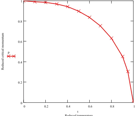
With P0 known, it is convenient to solve (19) in terms of the reduced (or normalized) variables defined as
c
t T T and p t( )P t Pc( ) 0. Figure 1 gives the re-sults of this exercise for 0 ≤t≤ 1. We have also studied the variation of p with t for five other elements: Pb, Hg, In, Tl, and Nb—by taking for their EFs the values given by the free electron model [20, p. 248], and found it to be similar to that of Sn.
p
t
0 0.2 0.4 0.6 0.8 1
0 0.2 0.4 0.6 0.8 1
Reduced temperature
[image:5.595.308.537.496.693.2]Reduced critical momentum
4. Equations for
Pc
(
T
,
H
= 0) and
Pc
(
T
= 0,
H
= 0) for a Non-Elemental SC
The Tcs and the multiple gaps of several non-elemental high-Tc SCs (other than iron-pnictide SCs) have been dealt with in [17,18] via GBCSEs. We recall from [13,16] that these equations constitute a generalization of the BCS equations because: 1) they incorporate the mecha- nism of multi-phonon exchanges for the formation of Cooper pairs besides the usual one-phonon exchange mechanism; and 2) they invoke more than one Debye temperature—which is another way to specify the mass- dependent Debye frequency of an ion species—to char- acterize the SC.
In order to calculate Pc in the scenario in which CPs are bound via say, two-phonon exchange mechanism in a CS AxB1-x, we need to generalize (19) and (24). This is accomplished by replacing the propagator in (12) by a superpropagator [13]:
1 2 3 1,2 1,2 2 2 1,2 , 2πrange of V :
or or
2 , 2
2 2
0, otherwise
q p
P p q P p q
c c c ab c c F D c F D V V I E m m E (35)
where 1,2 are the BCS model interactions for the species of phonons belonging to A, B in the combined state of the constituents A and B, to be distinguished from
1,2, which are the free state interactions of A, B;
0
c
V
c
V
c
,
1,2
D are to be similarly distinguished from 1,2. Following now the sequence of steps between (8) and (24), we obtain the generalized version of (19) as:
c D
1 1 2 01
d x J x J x (36) where
1 1 2 2 1 2 0 2 2 0 , , d 2 8 , , d 2 8, , tanh tanh
2 2 c c c c U c c U c c x P J x p m x P J x p m c
x P P x
P x
c
(37)
1,2 0 1,2, U1,2 1,2 c c
D c
N V P x.
Equation (24) now goes over to
1 1 D 1, , , , 0 2 2 D 2 0 0,
c c
c p c p
(39) where0 0
1 1
1
2 1 2
1 2 2 ln ln 8 8 ln P P E E
E E E m m
E E E (40)
1 1, 2 ;
c D
E E P0
2
is obtained from 1 by putting 1
. c D 2
The solution of (39) for MgB2, for example, requires the inputs of
E
1,2
c
and the two Debye temperatures:
1,2c
1,2B D D
k c
; in addition, we require EF of the CS. Such solutions will be addressed else where n puts of 1,2
c
and the two Debye temperatures:
1,2c
1,2cB D D
k ; in
addition, we require EF of the CS. Such solutions will be addressed elsewhere.
5. Discussion
We have dealt above with equations that were obtained via positive energy projection operators (PEPOs). This suffices for the problem addressed because Pc corre- sponds to the situation when W = 0; in this limit, it has been shown in [21] that the equation obtained via the negative energy projection operators is identical with the one obtained via the PEPOs; also that: 1) CPs formed via electron-electron and hole-hole scatterings make equal contributions to the BS amplitude; and 2) the amplitudes for the formation of CPs corresponding to the mixed en- ergy projection operators are zero.
Note that if we concern ourselves with the ratios of jcs at different temperatures, which seems to be a realistic application of our equations, then the choice of the effec- tive mass of the electron in (1) becomes immaterial.
Even a cursory survey of the literature shows that jc of an elemental/non-elemental SC can vary between wide limits—depending upon the shape, size and alloying ma- terials of the sample. The study presented here suggests that this variation comes about because each sample has its own set of intrinsic parameters: Tc, θD, and EF. Sub- stituting these into the equation for jc (which is known from experiment) leads to a relation involving ns and EF. Knowledge of either of them then determines the other.
We finally note that the equations for jc(T) presented in this paper can be generalized to include an external mag- netic field via the Landau quantization scheme—as has been done to obtain dynamics-based equations for critical magnetic fields for both elemental and non-elemental
SCs in [22].
6. Conclusions
Equation (19) for an elemental SC and (36) for a non- elemental SC are the new results of this paper: they en-able one to calculate the critical momentum Pc of the SC at any T in zero-external magnetic field directly in terms of the familiar parameters [N(0)V], D and EF that characterize it. Substitution of these values of Pc into (1) then constitutes a direct approach for the calculation of the critical current densities.
T = 0 limits of both (19) and (36) were obtained— leading to (24) and (40), respectively. While it was fur- ther shown that (24) can justifiably be reduced to (25), we note that caution needs to be exercised should one seek to carry out a similar reduction of (40).
A necessary input for the calculation of Pc (and hence
jc) of an SC is its EF, which is a parameter that is seldom available for the high-Tc SCs. It therefore seems to us that an immediate and realistic application of the ap- proach presented here is to calculate the EF of such SCs via the input of their jcs which are readily available in the literature. The importance of EF of the high-Tc SCs is borne out by the studies reported in [6] and [8-12].
7. Acknowledgements
The author acknowledges correspondence with Professor M. de Llano and Professor D. C. Mattis having a bearing on this submission. He is grateful to Professor A. N. Mi- tra for continued encouragement.
REFERENCES
[1] M. Randeria, “Crossover from BCS Theory to Bose-Ein- stein Condensation,” In: A. Griffin, D. W. Snoke and S. Stringari, Eds., Bose-Einstein Condensation, Cambridge University Press, Cambridge, 1995, p. 355.
doi:10.1017/CBO9780511524240.017
[2] M Tinkham, “Introduction to Superconductivity,” McGraw Hill, New York, 1975.
[3] H. Ibach and H. Lüth, “Solid State Physics,” Springer, Berlin, 1996. doi:10.1007/978-3-642-88199-2
[4] C. P. Bean, “Magnetization of High-Field Superconduc- tors,” Reviews of Modern Physics, Vol. 36, No. 1, 1964, pp. 31-39. doi:10.1103/RevModPhys.36.31
[5] Y. B. Kim, C. F. Hempstead and A. R. Strand, “Magneti- zation and Critical Supercurrents,” Physical Review, Vol. 129, No. 2, 1963, pp. 528-535.
doi:10.1103/PhysRev.129.528
[6] A. S. Alexandrov, “Nonadiabatiic Superconductivity in MgB2 and Cuprates,” 2001.
http://arxiv.org/abs/cond-mat/0104413
[7] A. P. Cracknell and K. C. Wong, “The Fermi Surface,” Clarendon Press, Oxford, 1973.
[8] J. C. Campuzano, G. Jennings, M. Faiz, L. Beaulaigue, B. W. Veal, J. Z. Liu, A. P. Paulikas, K. Vandervoort, H. Claus, R. S. List, A. J. Arko and R. J. Bartlett, “Fermi Sur- faces of YBa2Cu3O6.9 as seen by Angle-Resolved Photo-
emission,” Physical Review Letters, Vol. 64, No. 19, 1990, pp. 2308-2311. doi:10.1103/PhysRevLett.64.2308
[9] C. G. Olsson, R. Liu, D. W. Lynch, R. S. List, A. J. Arko, B. W. Veal, P. Z. Jiang and A. P. Paulika, “High-Resolu- tion Angle-Resolved Photoemission Study of the Fermi Surface and the Normal-State Electronic Structure of Bi2Sr2CaCu2O8,” Physical Review B, Vol. 42, No. 1, 1990,
pp. 381-386. doi:10.1103/PhysRevB.42.381
[10] D.-H. Lee, “Iron-Based Superconductors: Nodal Rings,”
Nature Physics, Vol. 8, 2012, pp. 364-365.
doi:10.1038/nphys2301
[11] Y. Zhang, Z. R. Ye, Q. Q. Ge, F. Chen, J. Jiang, M. Xu, B. P. Xie and D. L. Feng, “Nodal Superconducting-Gap Stru- cture in Ferropnictide Superconductor BaFe2(As0.7P0.3)2,”
Nature Physics, Vol. 8, 2012, pp. 371-375.
doi:10.1038/nphys2248
[12] M. P. Allan, A. W. Rost, A. P. Mackenzie, Y. Xie, J. C. Davis, K. Kihou, C. H. Lee, A. Iyo, H. Eisaki and T.-M. Chuang, “Anisotropic Energy Gaps of Iron-Based Super- conductivity from Intraband Quasiparticle Interference in LiFeAs,” Science, Vol. 336, No. 6081, 2012, pp. 563-567.
doi:10.1126/science.1218726
[13] G. P. Malik, “On the Equivalence of the Binding Energy of a Cooper Pair and the BCS Energy Gap: A Framework for Dealing with Composite Superconductors,” Interna- tional Journal of Modern Physics B, Vol. 24, No. 9, 2010, pp. 1159-1172. doi:10.1142/S0217979210055408
[14] G. P. Malik, I. Chávez and M. de Llano, “Generalized BCS Equations and Iron-Pnictide Superconductors,” Jour- nal of Modern Physics, Vol. 4, 2013, pp. 474-480. [15] E. E. Salpeter, “Mass Corrections to the Fine Structure of
Hydrogen-Like Atoms,” Physical Review, Vol. 87, No. 2, 1952, p. 328. doi:10.1103/PhysRev.87.328
[16] G. P. Malik and U. Malik, “High-Tc Superconductivity
via Superpropagators,” Physica B, Vol. 336, No. 3-4, 2003, pp. 349-352. doi:10.1016/S0921-4526(03)00302-8
[17] G. P. Malik, “Generalized BCS Equations: Applications,”
International Journal of Modern Physics B, Vol. 24, No. 19, 2010, pp. 3701-3712.
doi:10.1142/S0217979210055858
[18] G. P. Malik and U. Malik, “A Study of the Thallium- and Bismuth-Based High-Temperature Superconductors in the Framework of the Generalized BCS Equations,” Journal of Superconductivity and Novel Magnetism,Vol.24, No. 1-2, 2011, pp. 255-260. doi:10.1007/s10948-010-1009-0
[19] A. C. Rose-Innes and E. H. Rhoderic, “Introduction to Su- perconductivity,” Pergamon, Oxford, 1978.
[20] C. Kittel, “Introduction to Solid State Physics,” Wiley Eastern, New Delhi, 1974.
pagators Revisited,” Physica C, Vol. 468, No. 13, 2008, pp. 949-954. doi:10.1016/j.physc.2008.03.002
[22] G. P. Malik, “On Landau Quantization of Cooper Pairs in
a Heat Bath,” Physica B,Vol. 405, 2010, pp. 3475-3481.