Quality Assessment of MODIS Time Series Images and the Effect on Drought Monitoring

http://www.scirp.org/journal/ojapps ISSN Online: 2165-3925

ISSN Print: 2165-3917

Quality Assessment of MODIS Time Series

Images and the Effect on Drought Monitoring

Hedia Chakroun

National School of Engineering of Tunis, University of Tunis El Manar, Tunis, Tunisia

Abstract

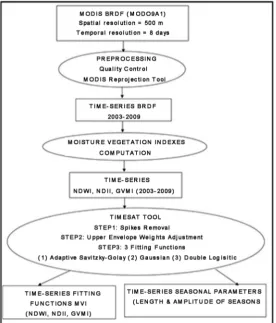
Drought Monitoring by remotely sensed moisture vegetation indexes is being an active research subject as the vegetation spectral responses are showed to be highly correlated to water content. The MODIS (MODerate resolution Imaging Spectro-radiometer) sensor of the Terra satellite provides MOD09A1 product of BRDF (Bidirectional Reflectance Distribution Function) used in computing moisture vegetation indexes (MVI). The exploration of an MVI time-series in the Kroumirie forest in Northern Tunisia showed important noise due to both clouds contamination and sensor defaults that had to be removed. Amongst methods for removing these imperfections, TIMESAT tool was designed for correcting time-series of satellite data and also to retrieve seasonal parameters from smoothed vegetation indexes. The methodology of smoothing functions to fit the time series data is based on two stages. First, a least square fit to the upper envelope of the vegetation indices series is ap-plied. The second stage is achieved by local and adaptive fitting functions. The corrections have been made by spikes removal due to abrupt change of MVI variations and by fitting the MVI time-series to the upper envelop to correct the negative biases of remote sensing vegetation indexes. The adaptive Savitsky- Golay function filter compared to local filtering process produces variations that conserve local variations for all the tested MVI. Seasonal vegetation pa-rameters were extracted for each year of the time-series analysis and com-pared to the Standardized Precipitation Index (SPI) calculated at meteorolog-ical station level and for different time scales. Positive relations were found between SPI and the seasonal parameters expressed by the length and the am-plitude of the season, indicating MODIS derived MVI sensitivity to water def-icit or surplus conditions. The 6-month SPI showed the best performance when related to water sensitive indexes suggesting that MODIS derived in-dexes are more correlated to the precipitation variations over seasons.

Keywords

MODIS Time Series, Moisture Vegetation Indexes, TIMESAT, Drought, SPI,

How to cite this paper: Chakroun, H. (2017) Quality Assessment of MODIS Time Series Images and the Effect on Drought Monitoring. Open Journal of Applied Sci- ences, 7, 365-383.

https://doi.org/10.4236/ojapps.2017.77029

Received: June 14, 2017 Accepted: July 22, 2017 Published: July 25, 2017

Copyright © 2017 by author and Scientific Research Publishing Inc. This work is licensed under the Creative Commons Attribution International License (CC BY 4.0).

Mediterranean Forests

1. Introduction

Global and regional monitoring of drought is becoming an active research sub-ject to determine the impacts of drought on water management and socio-eco- nomic development, especially in limited water resources regions where drought episodes highly control water availability and functioning of forested and culti-vated ecosystems. Various approaches for drought definitions and drought in-dexes were developed and synthesized in review studies such as [1]. On the other hand, during the last two decades, the models used in the assessment of drought causes and manifestations integrated more and more indicators from multi- sensors satellite images to study their correlation with drought indexes. The monitoring of vegetation moisture by remote sensing became an active research subject in various studies within natural and cultivated areas where the vegeta-tion spectral responses are showed to be highly correlated to physical indicators of water content and consequently to drought episodes. These studies that are based on linking spectral vegetation response to meteorological drought indexes, and are carried out to overcome sparse and inadequate network of weather sta-tions. For example, [2] proposed a comprehensive analysis to evaluate the per-formance of remote sensing data towards drought conditions for fire prone ve-getation in Australia. In [3] spectral vegetation response with thermal images and TRMM precipitation images (Tropical Rainfall Measuring Mission) was in-tegrated in a unique drought spectral index that had been shown to be correlated with drought indexes such as SPI (Standardized Precipitation Index) and varia-tion of crop yield in China. In the southern shore of the Mediterranean basin known as one of the most exposed regions to climate changes [4], there is a need of consistent drought monitoring to ensure a balanced ecohydrological func-tioning and to help mitigate climate changes effects. In [5] hydric stress and drought impacts on ecohydrologic balance were studied in a forested ecosystem of northern Tunisia.

spatial resolution SPOT-VEGETATION program launched in the nineties. Since the early 2000 s, the availability of MODIS products has brought a breakthrough in time-series data with the 250-m spatial resolution NDVI product (MOD- 13Q1). Many studies assessed the performance of MODIS (MOD erate resolu-tion Imaging Spectro-radiometer) as a keystone satellite sensor system providing multiple products, such as MOD09A1 product, a near-daily coverage of the Earth surface, at 500 m in visible and infrared ranges. This product has also the advantage of two narrow discrete channels in the SWIR bands with a signal to noise ratio above 100 [7] which both could be useful for the monitoring of leaf water content [8]. MODIS bands 5, 6 and 7 are well suited for canopy water monitoring because of the plant water sensitivity in these wavelengths combined with the high atmospheric water vapor transmittance [9].

Despite the wide use of MODIS sensors, many users reported that MODIS time-series can be subject to errors due to gaps, clouds and noise (e.g. [10][11] [12]). Therefore an adequate use of this product requires a correction of re-motely sensed time-series data. Amongst the various approaches of time-series images smoothing, local and global fitting methods are widely used. Local fitting methods are based on surrounding value of data in a time-series determined by median smoothing approaches [13] or by Savitzky-Golay filter approach [14] [15]. Global approaches fit the data to long time scale of observations such as Fourier transform used in frequency analysis of a signal (for an extended review of filtering methods, refer to [11]). The elimination of noise by filtering process allow san estimation of vegetation seasonal patterns such as the length of the season and the seasonal amplitude. Therefore, most of time-series smoothing algorithms are compared for their phonologic metric detection such as start and end of the season [16] [17]. They also could bring valuable information on drought occurrence as addressed in [18] where Fourier transform was used on a time-series of NDVI to identify specific frequency components corresponding to dry years.

In the present study, local approaches are tested within the tool TIMESAT developed by [15]. This tool was used in various time-series filtering (e.g. [11] [12][19]). Our main objective was to compare different smoothing algorithms of time-series moisture vegetation indexes computed from MODIS spectral bands in a forested Mediterranean region of northern Tunisia. These algorithms are embedded in the TIMESAT software that was used principally for anomalies corrections of the vegetation indexes time-series. Fitting functions used in the different algorithms allow the determination of the start and the end of vegeta-tion season in the study region. We hypothesized that these comparative outputs of the season length and the amplitude reached by vegetation indexes could be adequate indicators of vegetation response to water deficits or surplus when compared to the SPI drought index.

filtering functions to make necessary corrections of the imperfections of the used data; 3) to determine the vegetation seasonality parameters for the years of the time-series of the study; 4) to investigate the relationship between seasonal pa-rameters derived from filtered MVI time-series and the drought meteorological index SPI within the study ecosystem.

2. Study Area

The research focuses on the northern ecoregion of Tunisia known as the Kroumirie Forest, belonging to the Mediterranean North African forests (7˚52'E-37˚29'N to 9˚33'E-36˚22'N) (Figure 1). This ecoregion covering an area of 255,000 ha, is characterized by deciduous forest mostly represented by tree layer of cork oak (Quercus suber), shrub layer (e.g. Erica arborea and Pistacial entiscus) and herbaceous litter layer. This region has an average annual precipi-tation of 700 mm, but locally, precipiprecipi-tation can reach 1500 mm [20]. Isohyets of annual average precipitation illustrated in Figure 1 show an important gradient of precipitation decrease in the direction NW-SE. The Mediterranean climate of the study region is characterized by rainy autumns and winters where precipita-tions are distributed between September and March.

The deciduous forest of Kroumirie region is highly detected by MODIS sen-sors. The processing of the Enhanced Vegetation Index (EVI) (MOD13Q1 bi-weekly product: 250 m spatial resolution) allows the discrimination of agri-culture (EVI < 0.1) and forested areas that we classify in 3 density classes as illu-strated in Figure 1.

Figure 1. Map of the Kroumirie Forest ecoregion showing the vegeation density

3. Times-Series Precipitation Data and MODIS Images

The analysis period targeted in the present study covered the years between 2003 and 2009. Both 8-daystime-series of MODIS images and daily precipitations of four meteorological stations within the study region were acquired and proce- ssed. Meteorological data were available in four stations (illustrated in Figure 1) between 2002 and 2009, whereas MODIS images were available since 2003.

3.1. Drought Assessment by SPI

The Standardized Precipitation Index (SPI) [21], is a common measure of me-teorological drought calculated from in-situ precipitation data registered at a given station. SPI calculation requires monthly precipitations at a local station to capture the cumulated deficit or surplus of precipitations over a given timescale. SPI is based on fitting the total time-series precipitation to a gamma probability density function and, transforming the gamma distribution to a normal distri-bution with zero as mean and 1 as standard deviation. Values of SPI allow the characterization of the meteorological drought in a station as this index represents the number of standard deviations of an observed precipitation from the long term mean precipitation value calculated for a long term period. On the basis of computed SPI values, a drought category is associated to the station as shown in Table 1. SPI can be estimated at a station level for different time scales (3 months, 6 months, 12 months and more) and for each month of the year. 3-month SPI provides short and medium-term moisture conditions whereas 6-month SPI shows effects over seasons. 12-month SPI and more are used to analyze long term precipitations patterns.

In the Kroumirie region, records of four meteorological stations were used to calculate the SPI from monthly precipitations of the period 2002-2009, except for Feija station where records of 2002-2003 were missing (Figure 2).

3.2. MODIS Time-Series Data

The MOD09A1 product of the BRDF corresponds to 8 days with a spatial reso-lution of 500 m. Images corresponding to the period 2003-2010 were

Table 1. Drought classification based on SPI ranges [21].

SPI range Drought category

>2 Extremely wet

1.5 to 1.99 Severely wet

1.0 to 1.49 Moderately wet

0.99 to 0 Mildly wet

0 to -0.99 Mild drought

−1.0 to −1.49 Moderate drought

−1.5 to −1.99 Severe drought

Figure 2. Annual precipitations in meteorological stations of the Kroumirie forest. (Data source: DGRE: General Department of Water Resources).

provided as Hierarchical Data Format-Earth Observing System (HDF-EOS) downloaded from the online USGS Global Visualization Viewer (GloVis) [22]. Data were selected and ordered within a graphical interface. Tiles covering North Africa region were clipped to the extent of Tunisia. The images were rec-tified from sinusoidal projection to geographic projection by the use of MODIS Reprojection Tool, and next they were converted to Universal Transverse Mer-cator (UTM, zone 32 North). From visualization and profiles examination, we noticed important noise due to clouds contamination or sensor defaults that had to be removed. We also noticed that band 5 of the MOD09A1 product presents a regular strip effect.

Monitoring of vegetation moisture is possible through water sensitive indexes (MVI) based on BRDF combination in the various spectral wavelengths. The most used MVI reported in the literature are 1) NDWI: Normalized Difference Water Index [8], 2) NDII: Normalized Difference Infrared Index [23], and 3) GVMI: Global Moisture Vegetation Index [24]. These MVI were developed from the combination of the near infrared (NIR) (B2 of MOD09A1) and the SWIR (B5, B6 and B7 of MOD09A1); the latter are particularly sensitive to the water content of vegetation [25] as shown in Figure 3.

In a previous research in the Kroumirie forest comparing field moisture data with MVI computed from MODIS [26], it has been shown that MVI are highly correlated to vegetation water content in this ecosystem. In other water limited ecosystems, a study led in Australia confirmed that MVI are sensitive to drought intensity and are highly correlated to SPI [27]. The expression of the various MVI of the present study is given in Table 2.

4. Smoothing of MVI Time-Series by TIMESAT

Figure 3. Leaf spectral reflectance simulated for MODIS and LANDSAT bands. Response in SWIR bandsis sensitive to relative water content (RWC) [25].

Table 2. Moisture vegetation indexes based on MODIS spectral bands (MOD09A1).

MVI (Moisture Vegetation Indexes) NDWI = (B2 − B5)/(B2 + B5) NDII6 = (B2 – B6)/(B2 + B6) NDII7 = (B2 − B7)/(B2 + B7)

GVMI6 = [(B2 + 0.1) − (B6 + 0.02)]/[(B2 + 0.1) + (B6 + 0.02)] GVMI7 = [(B2 + 0.1) − (B7 + 0.02)]/[(B2 + 0.1) + (B7 + 0.02)]

4.1. Methodological Stages of TIMESAT

The methodology of smoothing MVI time-series by TIMESAT is based on three stages to accomplish the correction of the synthesized as follows:

The first step is based on a preliminary processing of data; it is applied to re-move values of MVI corresponding to abrupt changes (spikes). This processing makes use of quality data available as additional band with the MODIS product.

Secondly, a least square fits to the upper envelope of the MVI is used to over-come the fact that vegetation indexes generated from remotely sensed data are negatively biased as proved for example for NDVI (Normalized Difference Ve-getation Index) time series by [29].

Figure 4. Flowchart of MODIS time-series processing in TIMESAT.

(a) (b)

Figure 5. Fitted functions to the upper envelope of NDVI time series. Thin solid line

reprsents the original vegetation index data and the thick line displays the fitted function. (a) Fitted function from the first weights; (b) Fitted function from decreased weights for low NDVI [30].

procedure. The first step results in a fitted function affected by original lowest values of NDVI Figure 5(a), whereas Figure 5(b) shows the effect of low data weight decrease on the final fitted function.

4.2. Filtering Methods

The filters in TIMESAT tool are of two types: 1) local model fitting based on mi-nima and maxima, and 2) adaptive filtering.

In the first case, data are fitted to local model functions defined in intervals around maxima and minima in the time-series data. The local model functions have the general form given by Equation (1). The local fitting function uses two types of functions which are: the asymmetric Gaussian function Equation (2) and the double logistic function Equation (3).

( )

( )

f t = +c c g t x (1)

where (c1, c2) determine the base level and the amplitude of the fitting function f(t), “x” is the non linear parameter determining the shape of the basis function and “t” is the time variable.

(

)

1 2 5

1

1 4

exp if

; , , ,

exp if

x x t t x t x x

g t x x x

x

t x

x

−

  _{ − } 

 −   >

        =     _   _ − <         _{ } 

 (2)

where “x1” determines the position of the maximum or minimum with respect

to the independent time variable t, (x2, x3) determine the width and flatness of

the right function half, (x4, x5) determine the width and flatness of the left

func-tion half.

(

)

1 3

2 4

1 1

; , , ,

1 exp t 1 exp t

g t x x x

x x x x − − = −     + _{ } + _{ }    

 (3)

where “x1” determines the position of the left inflection point, “x2” gives the rate

of change, (x3, x4) give the same parameters for the right inflection point.

The second method is known as the adaptive Savitzky-Golay SG filter ([31] [32]) and uses a linear combination of nearby values in a window to fit locally a polynomial function by a least square method. The filtered value is then calcu-lated to fit to a polynomial function while varying locally the size of the window to avoid getting very important variations between original value and filtered value. For a VI time-series, if we assume that at a date “t”, VI(t) is noted yi, this yi is replaced by a linear combination of nearby values of a window where “n”

represents the size of the window. Equation (4) gives the SG filtered value of

yi:

( )

n

i filtered j n j i j

y =

∑

where yi is the original data series representing one date value of VI, Cj is the

weight of the jth _{original data value y}

j in the smoothing window size equal to (2n

The window size “n” can be adjusted to avoid obtaining large variations around a given VI value.

4.3. Seasonal Vegetation

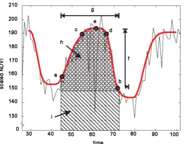
Considering a time-series of VI with one growing season per year, seasonality parameters resulting from fitting functions can be extracted for each full season of the time-series. Various parameters could be computed from the filtered MVI as shown in Figure 6: the start, the end and the length of the season; the seasonal amplitude and the integral of the function describing the season. These seasonal parameters allow the comparison of the vegetation response to water availability offering the possibility to investigate and explain inter-annual variations of the ecosystem vegetation status over space and time.

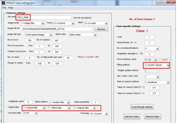
4.4. Setting of TIMESAT Parameters

The parameters that need to be set in the beginning of time-series filtering by TIMESAT are illustrated by the interface example of Figure 7. The main para-meters that have to be specified are:

• _{Amplitude cutoff value: time-series with smaller amplitude than the cutoff}

will not be processed; this parameter could be set to 0 to process all data.

• _{Spike method: the median filter method assigns a zero weight to values that}

are substantially different from both the left and right-hand neighbors and from the median in a window. The difference from the median is measured in units of the standard deviation of the time-series that we set to 2 (“Spike Parameters” =2).

• _{Number of envelope iterations: this setting allows two additional fits where}

the weights of the values below the fitted curve is decreased forcing the fitted function toward the upper envelope.

Figure 6. Seasonality parameters extraction. Points (a) and (b)

Figure 7. An example of parameters setting for filtering an NDII6 eight years time-series in TIMESAT tool.

• _{Adaptation strength: this number indicates also the strength of the upper}

envelope adaptation. After some trials, we set the value 3 for envelope itera-tions and the strength adaptation was set to 2.

5. Results and Discussion

5.1. Analysis of MVI Time-Series Filtering

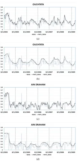
The moisture vegetation indexes MVI were computed from the BRDF product covering the time-series period from January 2003 to December 2010. In each year, 46 images were acquired and processed on the basis of one image each 8 days. Thus the total images proceeded in this data set are 368. Next, each time- series vegetation index had been processed in TIMESAT where local and adap-tive filtering functions were tested. Results were first analyzed based on visual exploration of time-series profiles at various locations in the Kroumirie Forest region. Figure 8 shows original data and the three fitting functions of the NDII6 time-series for “Ain Draham” and “Ouchtata” sites representing maximum and minimum time-series annual precipitation. The other MVI (non illustrated here) represent the same patterns of fitting functions with variations in the maximum reached by the MVI and the amplitude of the function over time. Compared to original values of NDII6, the fitting function process eliminated the extreme values (spikes) resulting in sensor imperfection or clouds. Moreover, data were fitted to the upper envelope to compensate for the negative biases of vegetation indexes.

(a)

(b)

(c)

(d)

Figure 8. Time-series plot of NDII6 values. Adpative SG filter for

(a) Ouchtata (c)Ain Draham. Local filters for (b) Ouchtata (d)Ain Draham. (FMT1 is SG sadaptive filter; FMT2 is the asymmetric Gaussian function; FMT3 is the double logistic function.

The year 2003 presented the highest annual precipitations amongst the preci-pitation time-series as illustrated in Figure 2; this explains that computed MVI for this year show highest values compared to the other years.

5.2. Drought Analysis by SPI and MODIS Time Series

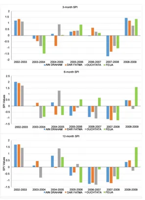
The SPI for four meteorological stations within the study region were computed for each month of the period where daily precipitations are available (2002- 2009), except for Feija station where records of 2002-2003 were missing. The SPI computed at the station level indicate that the study region experienced episodes of dry and wet conditions of different magnitude. To assess the possible relation between MVI derived from MODIS and drought intensity, the SPI values for the month of March were considered. For example, computation of 3-month SPI of March in a given year is based on the cumulative precipitations of January, Feb-ruary and March and it is compared to the same 3-month period of the time se-ries years. Figure 9 represents the SPI variations for 3, 6 and 12 months time scales showing the levels of drought affected to each station during the analysis period. From this analysis, we can conclude that the seasons 2002-2003 and 2008-2009 are the wettest ones, whereas for the other seasons, conditions were rather normal or moderately dry.

From smoothed MVI time-series by TIMESAT, the seasonal vegetation para-meters were extracted around the positions of the meteorological stations and compared to the SPI variations. The length of the season and the amplitude of the smoothed MVI vary from one year to another suggesting that water deficit/ surplus conditions influence the seasonal vegetation parameters. In particular, the integral of the MVI-function describing the season from the start to the end L-INTEG-MVI (denoted “h” in Figure 6) was extracted as it integrates both the amplitude and the length of the vegetative season, and could be an interesting indicator of precipitation deficit or surplus effects on the canopy.

For the explored stations, we noticed the existence of positive relations be-tween SPI and L-INTEG-MVI indicating that it is possible to make a monitoring of seasonal variation response to climate by remote sensing. As a first approxi-mation, a linear relation between SPI and L-INTEG-MVI was evaluated and the R2 _{coefficients were computed for each tested MVI (Table 3). Most significant}

results were obtained with 6-month SPI reflecting medium-term trends in preci-pitation and more rarely with 3-month SPI which reflects short-term moisture conditions. This suggests that water sensitive indices are more correlated to the precipitation variations over seasons.

Figure 9. SPI values for the period 2002-2009 calculated for 3, 6 and 12 months.

Table 3. Regression coefficients R2 _{of the linear relation between 6-month SPI (except}

underlined values obtained for 3-month SPI) and L-INTEG-MVI.

Station NDII6 NDII7 GVMI6 GVMI7 NDWI

AIN DRAHAM 0.78 0 0.79 0.67 0.74

DAR FATMA 0.56 0 0 0 0.80

OUCHTATA 0 0.45 0 0 0.40

FEIJA 0.6 0 0.43 0 0.83

In a second phase we tested a second degree relation between SPI and L- INTEG-MVI. Results reported in (Table 4) show that we have substantially the same relations but with increasing R2 _{coefficients. Figure 10 illustrates for each}

station the SPI and the time-course of the L-INTEG-MVI having the highest R2

coefficients.

Table 4. Regression coefficients R2 _{of the second degree relation between 6-month SPI}

(except underlined values obtained for 3-month SPI) and L-INTEG-MVI.

Station NDII6 NDII7 GVMI6 GVMI7 NDWI

AIN DRAHAM 0.91 0 0.79 0.67 0.98

DAR FATMA 0.91 0 0 0 0.99

OUCHTATA 0 0 0 0 0.77

FEIJA 0.66 0 0.46 0 0.97

Figure 10. SPI at multiple time scales and L-INTEG-MVI variation between

2003 and 2009.

rela-tively close in these bands (Table 2, Figure 3). On the other hand, the NDII and the GVMI indexes, computed from MODIS B2, B6 and B7, generate low but not zero values of L-INTEG-MVI for these years. The amplitude variation of L- INTEG-NDWI is small compared to that computed from NDII6, NDII7, GVMI6 and GVMI7 (Figure 10). Therefore, despite the high R2 _coefficients

val-ues obtained with first and second degree relations between SPI and L-INTEG- NDWI, this B5-based MVI is not recommended for vegetation response to cli-mate conditions in the study region.

From the previous analysis, our hypothesis that the season length and the am-plitude reached by remotely sensed vegetation indexes could be adequate indi-cators of vegetation response to water deficits or surplus is validated in the sites where SPI were calculated. It will be possible to improve these preliminary re-sults by spatial correlations between SPI extended to the whole region and the seasonal parameters extracted from the fitted MVI time-series fitted functions.

6. Conclusions

This study presented moisture vegetation indexes time-series corresponding to 8-days images acquired from 2003 to 2009 and calculated from MODIS spectral bands after anomalies corrections by filtering functions in TIMESAT tool. All the tested filtering functions had eliminated spikes and the time-series data were fitted to the upper envelope thus overcoming the negative biases of vegetation indices. Amongst the three methods tested in this tool, it has been shown that adaptive Savitzky-Golay fitting function is more appropriate because it simulta-neously corrects the imperfections represented by spikes while keeping the vari-ations due to a natural evolution of the moisture vegetation indices. Local filter-ing asymmetric Gaussian function and double logistic function capture less local variations; however they generate more obvious limits of start and end of vegeta-tive season.

Analysis of the SPI computed from an eight-year history (2002-2009) of pre-cipitation records demonstrated that smoothed moisture vegetation indexes have the capacity to detect wet and drought conditions characterized either by a deficit or a surplus of precipitations. Seasonal functions integrating both the amplitude and the length of the vegetative season were analyzed in comparison to the SPI within each station at different time scales. Regression coefficients of the (SPI, L-INTEG-MVI) linear and polynomial positive relations show different performances for the tested MVI, but at least one MVI performs for each tested station. Moisture vegetation indexes computed from MODIS short wave infra red bands 6 and 7 outperformed the index computed from band 5. The best agreement between drought index SPI computed for three time scales (3, 6 and 12 months) and the seasonal parameters were with 6-month SPI suggesting that MODIS derived indices are more correlated to the precipitation variations over seasons.

been addressed and verified in the Mediterranean peculiar ecosystem. The inter-est of remote sensing indexes lies in the fact that the information is already spa-tialized and allows a monitoring of an ecosystem response to drought conditions via time-series moisture vegetation indices after their corrections by adequate filtering methods. These preliminary results should be improved by in-situ data on seasonal parameters as well as spatial correlations between SPI and spectral vegetation indexes extended to the whole region.

Acknowledgements

The author wishes to thank the Ministry of Agriculture and Water Resources of Tunisia for providing climatic data (especially Mrs H. Ben Mansour from the DGRE). The author also thanks NASA Earth Science Enterprise for providing free MODIS images on the web. The author presents a special thank to the de-velopers of the TIMESAT tool from Lund University, Sweden.

References

[1] Mishra, A.K. and Singh, V.P. (2010) A Review of Drought Concepts. Journal of Hy-drology, 391, 202-216. https://doi.org/10.1016/j.jhydrol.2010.07.012

[2] Caccamo, G., Chisholm, L.A., Bradstock, R.A. and Puotinen, M.L. (2010) A Com-parative Analysis of MODIS Based Spectral Indices for Drought Monitoring over Fire Prone Vegetation Types. American Geophysical Union, Fall Meeting 2010, San Fransisco, 13-17 December 2010.

[3] Du, L., Tian, Q., Yu, T., Meng, Q., Jancso, T., Udvardy, P. and Huang, Y. (2013) A Comprehensive Drought Monitoring Method Integrating MODIS and TRMM Da-ta. International Journal of Applied Earth Observation and Geoinformation, 23, 245-253. https://doi.org/10.1016/j.jag.2012.09.010

[4] IPCC (2007) Working Group III Contribution to the Intergovernmental Panel on Climate Change Fourth Assessment Report Climate Change 2007: Mitigation of Climate Change.

http://www.ipcc.ch/publications_and_data/publications_ipcc_fourth_assessment_re port_wg3_report_mitigation_of_climate_change.htm

[5] Chakroun, H., Mouillot, F., Nasr, Z., Nouri, M., Ennajah, A. and Ourcival, J.M. (2014) Performance of LAI-MODIS and the Influence on Drought Simulation in a Mediterranean Forest. Ecohydrology, 7, 1014-1028.

https://doi.org/10.1002/eco.1426

[6] Atzberger, C., Klisch, A., Mattiuzzi, M. and Vuolo, F. (2014) Phenological Metrics Derived over the European Continentfrom NDVI3g Data and MODIS Time Series.

Remote Sensing, 6, 257-284. https://doi.org/10.3390/rs6010257

[7] Guenther, B., Xiong, X. Salomonson, V.V., Barnes, W.L. and Young, J. (2002) On-Orbit Performance of the Earth Observing System (EOS) Moderate Resolution Imaging Spectroradiometer (MODIS) and the Attendant Level 1-B Data Product.

Remote Sensing of Environment, 83, 16-30.

https://doi.org/10.1016/S0034-4257(02)00097-4

[8] Gao, B.C. (1996) NDWI—A Normalized Difference Water Index for Remote Sens-ing of Vegetation Liquid Water from Space. Remote Sensing of Environment, 58, 257-266. https://doi.org/10.1016/S0034-4257(96)00067-3

Index from MODIS near- and Shortwave Infrared Data in a Semiarid Environment.

Remote Sensing of Environment, 87, 111-121.

https://doi.org/10.1016/j.rse.2003.07.002

[10] Atzberger, C., Vuolo, F. and Klisch, A. (2015) Use of MODIS Temporal Signatures for Regional-Scale and Cover Mapping and Crop Status Monitoring: Activities at Buku University. IEEE Geoscience and Remote Sensing Society, the International Geoscience and Remote Sensing Symposium (IGARSS), Mailand, 26-31 July 2015. [11] Yuan, H., Dai, Y., Xiao, Z., Ji, D. and Shangguan, W. (2011) Reprocessing the

MODIS Leaf Area Index Products for Land Surface and Climate Modelling. Remote Sensing of Environment, 15, 1171-1187.

[12] Choler, P., Sea, W. and Briggs, P. (2010) A Simple Ecohydrological Model Captures Essentials of Seasonal Leaf Dynamics in Semi-Arid Tropical Grasslands. Biogeos-ciences, 7, 907-920. https://doi.org/10.5194/bg-7-907-2010

[13] Reed, B.C., Brown, J.F., VanderZee, D., Loveland, T.R., Merchant, J.W. and Ohlen, D.O. (1994) Measuring Phenological Variability from Satellite Imagery. Journal of Vegetation Science, 5, 703-714. https://doi.org/10.2307/3235884

[14] Chen, J., Jönsson, P., Tamura, M., Gu, Z., Matsushita, B. and Eklundh, L. (2004) A Simple Method for Reconstructing a High-Quality NDVI Time-Series Data Set Based on the Savitzky-Golay Filter. Remote Sensing of Environment, 91, 332-344. [15] Jönsson, P. and Eklundh, L. (2004) TIMESAT—A Program for Analyzing Time-

Series of Satellite Sensor Data. Computers and Geosciences, 30, 833-845.

[16] Shao, Y., Lunetta, R.S., Wheeler, B., Liames, J.S. and Campbell, J.B. (2016) An Eval-uation of Time-Series Smoothing Algorithms for Land-Cover Classifications Using MODIS-NDVI Multi-Temporal Data. Remote Sensing of Environment,174, 258- 265.

[17] Atkinson, P.M., Jeganathan, C., Dash, J. and Atzberger, C. (2012) Inter-Comparison of Four Models for Smoothing Satellite Sensor Time-Series Data to Estimate Vege-tation Phenology. Remote Sensing of Environment, 123, 400-417.

[18] Zribi, M., Dridi, G., Amri, R. and Lili-Chabaane, Z. (2016) Analysis of the Effects of Drought on Vegetation Cover in a Mediterranean Region through the Use of SPOT-VGT and TERRA-MODIS Long Time Series. Remote Sensing,8, 992.

https://doi.org/10.3390/rs8120992

[19] Nertan, A.T., Stancalie, G. and Mihailescu, D. (2011) Analysis of MODIS LAI Time- Series Using TIMESAT Software. Case Study Romania. International Conference on Current Knowledge of Climate Change Impacts on Agriculture and Forestry in Eu-rope COST-WMO, Topolcianky, 3-6 May 2011.

[20] Nasr, Z., Woo, S.Y., Zineddine, M., Khaldi, A. and Rejeb, M.N. (2011) Sap Flow Es-timates of Quercus suber According to Climatic Conditions in North Tunisia. Afri-can Journal of Agricultural Research, 6, 4705-4710.

[21] McKee, T.B., Doesken, N.J. and Kliest, J. (1993) The Relationship of Drought Fre-quency and Duration to Time Scales. Proceedings of the 8th Conference on Applied Climatology, Anaheim, 17-22 January 1993, 179-184.

[22] http://reverb.echo.nasa.gov/

[23] Hardisky, M.A., Klemas, V. and Smart, R.M. (1983) The Influence of Soil Salinity, Growth Form, and Leaf Moisture on the Spectral Radiance of Spartina alterniflora

Canopies. Photogrammetric Engineering and Remote Sensing, 49, 77-83.

[25] Hunt, E.R., Li, L., Yilmaz, L.T. and Jackson, T.J. (2011) Comparison of Vegetation Water Contents Derived from Shortwave-Infrared and Passive-Microwave Sensors over Central Iowa. Remote Sensing of Environment, 115, 2376-2383.

[26] Chakroun, H., Mouillot, F. and Hamdi, A. (2015) Regional Equivalent Water Thickness Modeling from Remote Sensing across a Tree Cover/LAI Gradient in Mediterranean Forests of Northern Tunisia. Remote Sensing, 7, 1937-1961.

https://doi.org/10.3390/rs70201937

[27] Caccamo, G., Chisholm, L.A., Bradstock, R.A. and Puotinen, M.L. (2011) Assessing the Sensitivity of MODIS to Monitor Drought in High Biomass Ecosystems. Remote Sensing of Environment, 115, 2626-2639.

[28] http://www.nateko.lu.se/TIMESAT

[29] Chen, J.M., Deng, F. and Chen, M. (2006) Locally Adjusted Cubic-Spline Capping for Reconstructing Seasonal Trajectories of a Satellite-Derived Surface Parameter.

IEEE Transactions on Geoscience and Remote Sensing, 44, 2230-2238.

https://doi.org/10.1109/TGRS.2006.872089

[30] Eklundh, L. and Jönsson, P. (2009) TIMESAT 3.0 Software Manual. Lund Universi-ty, Sweden.

[31] Savitzky, A. and Golay, M.J.E. (1964) Smoothing and Differentiation of Data by Simplified Least Squares Procedures. Analytical Chemistry, 36, 1627-1639.

https://doi.org/10.1021/ac60214a047

[32] Press, W.H., Teukolsky, S.A., Vetterling, W.T. and Flannery, B.P. (1994) Numerical Recipes in Fortran. Cambridge University Press, Cambridge.

[33] Hird, J.N. and McDermid, G.J. (2009) Noise Reduction of NDVI Time-Series: An Empirical Comparison of Selected Techniques. Remote Sensing of Environment, 113, 248-258.

Submit or recommend next manuscript to SCIRP and we will provide best service for you:

Accepting pre-submission inquiries through Email, Facebook, LinkedIn, Twitter, etc. A wide selection of journals (inclusive of 9 subjects, more than 200 journals)

Providing 24-hour high-quality service User-friendly online submission system Fair and swift peer-review system

Efficient typesetting and proofreading procedure

Display of the result of downloads and visits, as well as the number of cited articles Maximum dissemination of your research work

Submit your manuscript at: http://papersubmission.scirp.org/