Green to Grey China: Determinants and Forecasts of its Green Growth

Munich Personal RePEc Archive

Green-to-Grey China: Determinants and

Forecasts of its Green Growth

You, Jing and Huang, Yongfu

School of Agricultural Economics and Rural Development Renmin

University of China, UNU-WIDER

19 December 2013

Online at

https://mpra.ub.uni-muenchen.de/58101/

Green-to-Grey China: Determinants and Forecasts

of its Green Growth

Jing You

School of Agricultural Economics and Rural Development Renmin University of China,

and Department of Land Economy, University of Cambridge. Email: jing.you@ruc.edu.cn

Yongfu Huang

World Institute for Development Economics Research United Nations University (UNU-WIDER)

Email: Yongfu.Huang@wider.unu.edu

This version, August 2014

Abstract

This paper investigates the determinants of China’s green growth and its pathways in the future. We use the OECD conceptual framework for green growth to measure green growth rates for 30 provinces over the period 1998-2011. By estimating a spatial dynamic panel model at provincial level, we find that China has experienced green growth, but with slower speed in the sample period. The average green growth rate is forecast to decline first and then fluctuate around zero over the next two decades. There appears to be a conditional convergence in provincial green growth and positive spatial influence across neighboring areas, yielding a cap of the country’s level of green development in the future. Mass innovation financed by the government and green structural reforms achieved at firm level are likely to stimulate green growth, while political shocks in terms of reappointment of provincial officials could retard China’s progress to a green economy.

Key words: Green growth, spatial dynamic panel model, forecasting, China

JEL classification: O10, O13, C33, O53

 

The authors are grateful to very helpful comments from Bernard Fingleton and participants in the IAAE Annual Conference in Queen Marry, University of London and the WCERE in Istanbul, both in 2014. This research is supported by the Research Funds of Peking University – Lincoln Institute Center for Urban Development and Land Policy (2013-2014, Grant No.: FS20130901), and the Specialized Research Fund for the Doctoral Program of Higher Education, the Ministry of Education of China (Grant No.: 20130004120001). The usual disclaimer applies. 

1. Introduction

In the past three decades, China has achieved a great economic success. However, this economic wonder has come at a high price. China’s environment has deteriorated rapidly and China has actually become one of the largest carbon dioxide emitters in the world. Climate change has already exerted detrimental effects on China’s water resources, disturbed the natural ecosystems, led to the coastal sea level rise and imposed various social and economic costs on society. Luckily, the Chinese government has fully realized the seriousness of the challenge and attached great importance to the battle for CO2 emission reduction. For example, China has

committed itself to reducing its carbon intensity by 40-45% between 2005 and 2020. This is a very challenging target, and will require vigorous efforts and large-scale changes in all aspects of the economy.

developed countries, can a truly effective international framework of fighting climate change be possible.

However, unlike the EU, America, or Australia which have long engaged themselves in emission reduction efforts with comparatively well-developed environmental protection mechanisms and infrastructure in place, China still has a long way to go and is not up to the challenge yet. Measured against China’s emission reduction target, so far China’s cleaning-up-the-economy progress has been unsatisfactory. China’s lack of a systematic carbon emission mitigation enabling framework is at the root of the problem. Among the key factors that obstruct China’s low carbon development progress are: China’s lack of effective environmental laws and institutions to guide and protect its low carbon development efforts (Chen, 2011), insufficient public awareness of how to protect the environment (Munro, 2013) and limited knowledge of for example “circular economy” even among officials (Xue et al., 2010), inadequate financial and technological investments to boost its sustainable development (Lewis, 2010; Chen, 2011) and a lack of a well-established carbon market to facilitate carbon emission reduction activities (Lo, 2013).

Given the very short time between now and 2015 when China will acknowledge legally-binding emission reduction targets, China has to make extra efforts and make fundamental changes to all aspects of its economic, political and social life to be ready for 2015. Due to its large-scale economy and huge population, the green growth of China’s economy will be crucial, not only for its own sustainable future but also for global sustainability. 1

1 _{It is worth noting that sustainable development encompasses three pillars, namely, economic}

So far, the literature suggests that economic and social improvements, especially in terms of poverty alleviation, tend to go hand in hand while the relationship between economic development and environmental protection has demonstrated a different story, with current economic growth being achieved at huge cost in environmental degradation. The ever-worsening environment and the urgent development needs of the world’s poor, especially in developing economies, highlight the urgency and necessity for the world to grow greener while at the same time keeping, if not accelerating, its current growth pace. Luckily, such two different and seemingly-incompatible demands can be reconciled into the single idea of green growth, which concerns both short-term economic growth and long-term environmental sustainability.

According to Hallegate et al. (2011), green growth can be defined as “fostering economic growth and development, while ensuring that natural assets continue to provide the resources and environmental services on which our well-being relies”. Unlike the traditional pattern of economic growth, which has been achieved largely at the expense of the environment, green growth aims to achieve synergy between economic progress and environmental protection, which is vital to realizing the goal of sustainable development.2 As pointed out by Toman (2012), green growth emphasizes that strategic environmental policies can both promote environmental sustainability at low cost and lead to sustained economic growth. Maximizing the synergy between the traditionally-incompatible factors of economic development and environmental sustainability will improve the social and political acceptability of

2

environmental policies. Huang and Quibria (2013) find that the extent of green growth in a given country depends on its earlier green growth development and regional diffusion, its domestic learning or determination to achieve the national politically-desired target, and exogenous shocks.

Although the urgency and need for low carbon development is widely acknowledged, little is known about how to decarbonize China’s economy in an effective and timely manner or what the global impact might be. The existing literature focuses mainly on environmental problems or exploitation of natural resources in the Chinese context. For example, a large number of studies have investigated the relationship between economic growth and emission of various pollutants.3 Others calculate the country’s total factor productivity when natural resource constraints are binding (Chen and Santos-Paulino, 2013) and forecast China’s CO2 emissions (Auffhammer and Carson, 2008) or energy demand (You,

2013). Despite some sensitivity to which indicators have been used and sample periods, the general pattern documented by the existing studies is that the higher economic growth, the more pollution and energy demand.4 Nevertheless, to the best of our knowledge, no literature measures directly China’s capability and potential for “green growth” by reconciling economic and environmental aspects in a coherent and empirically computable framework. In this respect, this paper uses the OECD’s (2011) conceptual framework of green growth to provide the first empirical analysis for China. More specifically, the questions addressed in this paper are: (i) how China’s green growth evolves; (ii) what factors contribute to China’s green growth, in

3

E.g., Brajer et al. (2011) for the existence of the Environmental Kuznets Curve (EKC) for aggregated and disaggregated indices of air pollution; Cole et al. (2011) for industrial pollutants at the city level and different firm ownerships; Zhang et al. (2013) for the extended association with energy consumption, air pollution and air protection investment; Wang et al. (2011) and Fei et al. (2011) for CO2 emission and Wang and Watson (2010) for its pathways in the future.

particular from the perspective of green structural reforms; and (iii) the future of China’s green growth, in the light of recent experience.

With a dynamic spatial panel model, we detect a convergence across Chinese provinces. By forecasting China’s green growth in the following years/decades, this research investigates whether China’s existing environmental protection measures have yielded the desired results of green growth and whether China is on the right track towards achieving its set emission reduction target by 2020. This study will provide much needed evaluation of the effectiveness of China's current low carbon development policies and measures. It will also provide policy advice for the Chinese government in terms of transition from the current GDP-focused economic growth pattern to a green growth trajectory. Given the lack of widely-recognized measures of green growth in the literature, this study will deepen our understanding of how to measure green growth and contribute to the methodology of investigating country-specific green growth research.

The present study proceeds as follows. The next section introduces our dataset. In particular, we spell out our construction of China’s green growth rate which is compatible with the OECD framework. Section 3 sketches the dynamic spatial panel model. Section 4 reports estimation results to answer our research questions and provide discussion and explanations. Possible implications for policy making are suggested in Section 5.

2. Data

composed of four dimensions: the socio-economic context and characteristics of growth, environmental and resource productivity, natural asset base, environmental quality of life, and economic opportunities and policy responses.

[Figure 1]

OECD (2011) proposes 23 categories to describe the whole system and lists possible indicators for each dimension (see pp. 139-140 of OECD, 2011). Huang and Quibria (2013) apply Principal Component Analysis (PCA) to 22 indicators which are highly relevant, analytically sound and currently available and measureable by OECD (2011) to extract a Green Growth Index for 36 OECD countries plus BRIICS (Brazil, Russia, India, Indonesia, China and South Africa), and examine the correlates of national green development potential from the perspective of structural reform. Similarly, the present study selects comparable indicators for 30 Chinese provinces over the period 1997-2011. Table 1 lists detailed variable definitions and data sources.

[Table 1]

We then apply the PCA to our indicators. The first component explains 44%-57% of the variance of the green growth components in various study years. The green growth rate is calculated as the growth rate of provincial green index. Table 2 lists descriptive statistics for our constructed green growth rates and all independent variables used in following analyses.

[Table 2]

curve had moved toward the right-hand side until 2000, meaning that more provinces switched to positive green growth rates along with economic development over time and none of them experienced negative green growth in 2000. However, about 20% of provinces during the first half of the 2000s saw retarded green growth, as the c.d.f. curve slid to the left again and part of the curve was left of zero green growth rates. In the second half of the 2000s, the c.d.f. curve swung around zero, and essentially there was no further progress in green growth. The c.d.f. curve in 2011 was far left of that in 2000 and green development was retarded in two provinces (6.7%).

[Figure 2]

growth rate, even though its real GDP per capita had grown 2.4 fold from 1998 to 2011. If the current pattern continues, the current positive green growth rates in most provinces will be corroded further and even drop below zero.

[Figure 3]

We average provincial green development indices in each year to obtain China’s average green development level. The national green growth rate is then calculated based on the annual average green development level. As shown in Table 7 later in Section 4.2., China experienced high green growth rates (97.5% per annum) in 1999 and 2000. After accession to WTO in 2000, the annual green growth rate dropped sharply to 2.56%. It rebounded to 9.5% during the 2007-2009 financial crisis when recession happened in most developed and in the main developing economies. Recently green growth rate has declined again along with economic repercussion. East and west China experienced higher green growth compared to the central region compared to the central region as East had the benefit of a better living environment and West was endowed with more natural resources.

3. Methodology

3.1. Modeling spatial dynamics of green growth

We begin by estimating a naïve regression for the pooled cross section. The province

i’s green growth rate at time t, GI_it, is regressed on its own time lag and the lagged level of green development, GI_{i t, 1} :

0 1 , 1 2 , 1

it i t i t it

GI   GI _  GI _ 

      (1)

where the disturbances _it ฀ N





and three time periods lag of green growth rates being the excluded instruments for

, 1

i t

GI _

 . Then, we consider the possible inter-provincial influence in provinces’ green

development and insert a spatially lagged term into (1) to reflect the impact of i’s neighboring provinces’ green growth on its own growth trajectory:

0 1 , 1 2 , 1 1

N

it i t i t ij jt it

j

GI   GI _  GI _  w GI 



     



30 30

W _ is a matrix symbolizing the connections between provinces and thus,





, 1, ,30

i j  . Specifically, we define two kinds of spatial matrices for Eq. (2) to take care of possibly different influences across neighboring provinces. First, a contiguity matrix takes the form as:

1 if

0 if or

ij ij

ij d w

d i j

 

 

  _{ }

 (3)

where d_ij is the distance between provinces i and j in kilometers. Provinces i and j are

labeled as “neighbors” with wij 1 if the distance between them is less than the

threshold .5 Each row in W_{30 30} is normalized so that the sum of wij in row is one.

Row standardization addresses the issue raised by Plümper and Neumayer (2010) that the potential influences might become proportionally smaller for those who have a larger number of neighbors. Second, there might be the “decaying” effect: the longer

5

the distance between i and j, the less influence could diffuse. Empirically, the elements in this distance-decay spatial matrix are calculated as:6

1

if

0 if or

ij ij

ij

ij

d d

w

d i j





 _

  

 _{ }



(4)

Again, the final W_{30 30} in regression is row standardized. Eq. (2) can be estimated by maximum likelihood estimation (MLE) as Anselin (2007) and generalized two stage least square (GS2SLS) developed by Kelejian and Prucha (1998, 1999, 2004). GS2SLS consists of four steps: (i) estimating the parameter vector

 

by two stage least squares using the first and second order spatial lags





WZ W Z as

the excluded instruments;7 (ii) computing residuals e_{j n,} after transforming the model by the Cochran-Orcutt type; and (iii) estimating the transformed model by generalized moment conditions proposed in Kapoor et al. (2007).

So far we have examined pooled cross sections. Next, we exploit the panel data to better reflect provincial unobserved time-invariant factors that may affect their green growth trajectories. Controlling provincial fixed effects also helps us purge spurious spatial dependence, as the genuine interdependence across “neighboring” provinces may be overstated by similar growth strategies, economic structure, cultural

6

As a robustness check, we also experimented Column 9 of Table 4 with higher orders in the denominator, e.g., 1₂

ij

d where d=1,500km and the decaying speed of spatial dependence is accelerated

with longer distance than that of Eq. (4). ˆ declines to 0.039 and statistically insignificant. 7

and institutional environment shared by certain provinces.8 We first re-estimate Eq. (1) with provincial fixed effects:9

0 1 , 1 2 , 1

it i t i t it

GI   GI _  GI _ 

      (5)

where the composite error _it contains a province-specific time-invariant effect _i

and an i.i.d. normally distributed disturbance it ฀ N





As the

pooled cross section, Eq. (5) can be consistently estimated by the standard OLS after phasing out spatial dependence. Next, the interplay between neighboring provinces is inserted as:

0 1 , 1 2 , 1 1

N

it i t i t ij jt i it

j

GI   GI _  GI _  w GI  



     



where _it follows an independent but not necessarily identical normal distribution across i and t. As the pooled cross section, we implement the standard OLS, IV, and GS2SLS estimation with the instruments being the first two orders of the spatial lag term.11 We also adopt two additional methods to estimate Eq. (6), in an effort to obtain robust results. First, as Huang and Quibria (2013), we employ a spatially-corrected system generalized method of moments (Spatial SYS-GMM) developed

8

In addition, common shocks may also be mistaken as spatial dependence which induces an upward bias in the estimated spatial dependence (Plümper and Neumayer, 2010). We will control explicitly for time trend and weather and political shocks in Columns 3-4 and 7-8 of Table 5. Significant and positive spatial dependence can be reaffirmed.

9

The Hausman tests based on the specifications of Columns (5) and (9) in Table 4 show that the null hypothesis that there are no systematic difference between the fixed- and random-effects models is firmly rejected at 1% significance level.

10

Here our specification does not include time fixed effects. Given the relatively large T in our dataset, the number of instruments in IV, GS2SLS and SYS-GMM estimation will be easily higher than 50 even we just use at most the 3rd order time lags. Weak- and over-identification problems indicated by the F-statistics and Sargan tests always exist when we re-estimated Eqs. (5) and (6) with time fixed effects. Although using more instruments could improve efficiency, Jin and Lee (2013) warn that bias also arises in finite samples, making the inference inaccurate. We tried to balance the trade-off between variance and bias by controlling a natural logarithmic time trend rather than a full list of time fixed effects when identifying the determinants of green growth in Eq. (8). However, this is not immune to problems, but is rather at the expense of the assumption of increasing marginal effects of unobserved time effects on green growth rates.

11

initially by Arellano and Bover (1995) and Blundell and Bond (1998) and recently extended to spatial panel models by Elhorst (2010), while only using the 2nd and 3rd period lags of the spatial term as the excluded instruments.12

Second, assuming the i.i.d. normal distribution of _it, we apply Lee and Yu’s (2010a) transform approach for the MLE and obtain consistent estimation of individual effects in the finite sample. The data are transformed to the deviation from the time mean before estimation to eliminate the individual effects. Therefore, the effective sample size becomes N T











    

 





1 1 1

ln , , ln 2 ln

2 2 2

1 ln

T

v v

t v

N T N T

L T                  



β e e

I W

(7)

where * 





e I W Xβ Xβ is the residual vector at the maximizers.

As stated in Section 1, this paper also aims to identify correlates of China’s green growth. We proceed to regress the provincial green growth rates on additional controls in the vector X at t1, which helps mitigate the potential endogeneity problem:

0 1 , 1 2 , 1 3 1

1

N

it i t i t ij jt t i it

j

GI   GI _  GI _  w GI  _  



     



It is worth noting that we only include a few crucial structural variables in X_t1. The one reason for not controlling many variables such as demographic and macroeconomic changes (e.g., population growth and GDP per capita) pertains to our construction of GI. It has already incorporated many socio-economic aspects given its

definition, including data on population and GDP. Multicollinearity will arise if using them again as independent variables. The other reason is that we focus on whether certain structural reforms could facilitate green growth, considering that structural transformation has featured in China’s reform since 1978 and boosted economic growth. See Knight and Ding (2012) for a comprehensive empirical analysis and Zhu (2012) for a recent review.13 Given data availability and the components having appeared in GI, X_t1 includes innovation, green economic structural reforms (e.g., the output value from reutilization of industrial waste, the output value from total environmental protection industry, the high-tech firms’ output value and green trade openness), and possible political and natural shocks that may alter the provincial green footstep. Detailed definition and calculation of these variables have been listed in Table 2.

Based on the estimates of Eq. (8), we further study the marginal effects of various structural and shock variables on provincial green growth. In the presence spatial dependence, these variables could influence green growth directly or indirectly transmitted through spatial interaction across provinces. Specifically, according to LeSage and Pace (2009) and Elhorst (2013), we calculate the short-term total marginal effect of a unit change  in one correlate x_k simultaneous in all provinces as:

13

฀

_{ }

_

_

฀





1 , , 1, , , 1, , ,

i k i k

ik

k i k ik i k nk

GI GI

x

GI x x x x x

                       

x x u

  (9)

where u





is calculated in reduced-form

฀

_{ }

  



1

ˆ ˆ

, ,

k N k

N k

k Nk

GI GI

x x  

 _{ }            x x I W  .

Averaging Eq. (9) across all provinces i1,,N yields the average total marginal effect (ATME):

฀

_{ }

_

_

฀









1 1

1 1, 1,

1 1 1 1 1 1 , , , , , , 1 ˆ ˆ N N

i k i k

i ik i

N

k i k ik i k nk

i N N k N i j GI GI

N x N

GI x x x x x

N N          _                        









x x e

I W

 

(10)

The average total effect is made of two components. When changing x_k sequentially in each province, say for i first, we obtain the direct marginal effect as follows

฀

_{ }

_

_





1k, , i 1,k, ik i, i 1,k, , nk

k k i

ik

GI x x x x x

GI GI x                

x x  

(11)

Averaging the above province-specific direct marginal effect of x_k across all provinces gives our measure of average direct marginal effect (ADME):

฀

_{ }

_

_

฀









1 1

1 1, 1,

1 1 1 1 1 , , , , , , 1 ˆ ˆ = N N

k k i

i ik i

N

k i k ik i i k nk

i N k N i GI GI

N x N

GI x x x x x

N N      _                  









influence can be measured by the difference between the average total (Eq. 10) and direct (Eq. 12) marginal effects:





1 1 ˆ ˆ N N k N i j i j N  _     



In the long run where GIi t, 1  GIit  GIi* and

* , 1

1 1 1

N N N

ij j t ij jt ij j

j j j

w GI _ w GI w GI

  

    







฀

_{ }

_{ }









1

1 1

ˆ _ˆ ˆ

, , 1

k N k

N k

k Nk

GI GI

x x   

 _{ }             x x I W

 for k1 . Averaging it

across all provinces gives us the long-term ATME,





1 1 1 1 ˆ ˆ _ˆ 1 N N k N i j N  _{ }     _{ }   



Similarly, the long-term ADME and AIME are calculated as





1 1 ˆ ˆ _ˆ 1 N k N i N  _{ }    _{ }   







1 1 ˆ ˆ _ˆ 1 N N k N i j i j N  _{ }      _{ }   



3.2. Forecasting green growth

We precede forecasting green growth at the aggregate (country) level into the future. In line with Kholodilin et al. (2008) for Germany and You (2013) for China, we conduct recursively quasi out-of-sample forecasting.

In the first step, we estimate Eq. (6) based on the full sample and calculate the root mean square forecast error (RMSFE). Second, we use the first-step estimators and the observations in the last sample year 2011 to calculate the predicted green growth rate in 2012. In particular, we refer to the reduced form Eq. (6),

฀

_

_

_

_

1 1 ˆ

ˆ , ,ˆ

t _{N t t}

GI   GI_ GI_

  I  W  α β to obtain predictions. Third, based on ฀GI2012

new predicted observations in 2012 in the full sample. RMSFE for the entire sample period, including this new plugged-in sample year 2012, is calculated after estimation. Fourth, based on the up-dated estimators, we again calculate the predicted green growth in the last sample year 2013, ฀GI2013 and RMSFE for the entire time-spanned.

We repeat this 1-step recursive forecasting over two decades until 2031. We will compute RMSFE in accompany to every round of forecasting to inform model performance.

4. Estimation results and discussion

4.1. Dynamics and determinants of green growth

Table 3 presents various estimators for the benchmark regressions, Eqs. (1-2), based on the pooled cross-sectional data. A significantly negative estimated coefficient of

ΔGIi,t-1 documents a negative time dependence in green growth rate. A significantly

negative estimated coefficient of GGIi,t-1 irrespective of estimation methods heralds a

β-convergence of provincial green growth rates – a tendency also observed in OECD countries by Huang and Quibria (2013). The green growth rate would decline 16.8-30.4 percentage points if the initial green development level in the province is 1% higher than before. The speed of convergence is relatively high, ranging between 18.4% per annum in Column 5 and 36.2% per annum in Column 1. This means that it could take only 2.28-4.12 years to halve the gap between initial and the steady-state green development levels at the current rate of convergence.14 Moreover, this could be interpreted as a long-run convergence process recorded globally at 1-year intervals given the pooled cross sectional data in estimation (Arbria et al., 2008) and estimating

14

It is derived by the half-time equation (Caselli et al., 1996): 0.5 1 T

e

Eq. (2) with spatial dependence (Columns 2-7 of Table 3) cannot change this pattern of green growth. A positive ˆ in all columns suggests that that a higher green growth rate in one province tends to affect positively its surrounding regions at 1%-10% significance levels under the assumption of either identical influence from neighbors (binary spatial matrix) or weakening influence from farther neighbors compared to near neighbors (inverse-distance spatial matrix). The magnitude of this positive spatial dependence in the latter case (Columns 6-7 of Table 3) is 11%-18% smaller than that in the former (Columns 3-4 of Table 3), which is predictable given the assumption of decaying spatial influence in the inverse-distance matrix.15

[Table 3]

When considering province fixed effects and estimating Eq. (5), we find again negative signs for GGIi,t-1 with high significance levels (Column 1 of Table 4) but

with larger magnitude in absolute terms. In other words, the rate of convergence to a steady state increases to 23.4%-165% per annum (Columns 8-9, respectively). In comparison with the pooled cross section, this rate of convergence could be understood as a global process. The time dependence in green growth rate becomes smaller than that of the pooled cross section as a result of inclusion of province fixed effects.

[Table 4]

However, various tests for homoscedasticity in residuals, such as Hall-Pagan LM test, Harvey LM test, Breusch-Godfrey test, Wald test, and White test, are all firmly rejected at 1% significance level, indicating unignorable correlates to green growth that have been missed in the model specification. We further specify two

15

different processes of spatial dependence and estimate Eq. (6) in Columns 2-5 and 6-8 of Table 4, respectively. Positive spatial influence in the progress to green growth is confirmed again, while we lose statistical significance under the assumption of homogenous influence from all neighbors (Columns 2-4 of Table 4). In contrast, strong and positive spatial dependence in green growth rates is still statistically significant under a more flexible assumption of decaying spatial spillover.

Furthermore, by comparing RMSEs in Tables 3 and 4, we can find that all columns in Table 4 generate lower RMSEs and better goodness-of-fit in terms of higher R2. This implies that provincial time-invariant unobservables may also play an important role in explaining dynamics of its green growth. Based on Column 9 of Table 4 where there are a flexible assumption of decaying spatial dependence and a lower RMSE, we derive provincial fixed effects in Figure 4. Their non-trivial magnitude (6.2-9.86) means that models overlooking provincial fixed effects such as those in Table 3 may suffer from potentially severe omitted variable problems. We will return to the impact of overlooking provincial fixed effects when implementing forecasts in Section 4.3.

[Figure 4]

4.2. Determinants of green growth

The performance of different estimation strategies in Table 4 suggests that GS2SLS produce more efficient estimators compared the other four, while MLE results in the smallest RMSE and therefore would be most suitable for forecasting. Therefore, we use GS2SLS to estimate the determinant regression, Eq. (8). Table 5 reports the estimated coefficients.

There is again a strongly negative estimated coefficient of GGIi,t-1 under all

estimation strategies, indicating a conditional convergence process in provincial green growth. The speed of convergence is further enhanced to 141%-276% per annum compared to that in dynamic spatial model in Table 4. We also calculate three different marginal effects in Table 6, based on the estimates of Columns 7 and 8 of Table 5 which assume inverse-distance spatial matrix and incorporate all relevant correlates of green growth. High speed of convergence results in large ATMEs of initial level of green development (-0.946 to -7.411 in Columns 1 and 4 of Table 6). The Broadly significant and positive influence of green growth across neighboring provinces is also reaffirmed, except the MLE. However, its magnitude varies substantially between GS2SLS and MLE. The latter generates trivial spatial dependence without statistical significance. As a result, effects from neighboring provinces (AIMEs) dominate ATMEs under GS2SLS, while the marginal effects basically come from the province itself (ADMEs) under MLE.

[Table 6]

and 5.16 The estimated coefficients of government support are 0.03 and 0.05 at 10% significance level under binary and inverse spatial matrices, respectively. The above findings suggest that in general, the mounting innovation efforts bring at most moderate increases in green growth rates, although China has strong incentives for skills development and technological transfer and upgrading (Altenburg et al., 2008). Moreover, government support in innovation activities dominates this positive impact compared to corporate R&D investment.

Green structural reforms in terms of sectoral shift is proxied first by growth in technological markets our analysis. As shown in Columns 1 and 5 of Table 5, higher transaction volumes are correlated with higher green growth rates but without statistical significance. By contrast, the sectoral shift in the form of higher output value of high-tech firms significantly promotes green growth (Columns 2 and 6 of Table 5) though the marginal effect is trivial: 1% more output value produced by high-tech firms would only add 0.005-0.193 percentage points to the speed of green development in the short run and 0.006-0.142 in the long run.

It is in general found in the existing literature that trade is beneficial for environmentally in OECD countries, while not for SO2 and CO2 for non-OECD

countries (e.g., Managi et al., 2009) and newly industrialized countries where trade openness is a long-term normal good for economic growth only (Hossain, 2011). Kozul-Wright and Fortunato (2012) further summarize two channels through which trade affects carbon emissions. For one thing, developed countries, having set up high environmental standards and having to abate greenhouse gas emissions, could relocate production to developing countries through international trade (i.e., the pollution heaven hypothesis). When exposed to international markets, developing countries

would tend to protect their bottom line firms by lowering domestic environmental standards (i.e., race to the bottom hypothesis). For another, trade openness affects domestic environmental quality via its positive effect on economic growth.17 Domestic environment may deteriorate under the scale effect should trade openness propel economic growth. That is, expanded economic activities would require more resource input and produce more waste and pollutants (or an EKC). Environment may also be improved as a consequence of the technique and composition effects. The former argues that people would pay more attention to sustainable production patterns and firms would use cleaner production techniques. The latter states that people would have a stronger propensity to protect environment as wealth increases and the structure of the economy would be adjusted leading to different environmental pressures in the future.

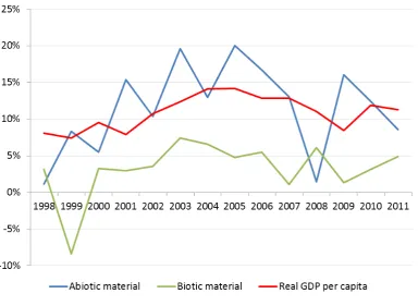
Taking the existing literature into account, we distinguish between the extent and degrees of green trade openness in our analyses. Although more exposure and access to international markets are found to contribute to China’s economic growth (Knight and Ding, 2012), the extent of green trade openness, proxied by the share of import and export of high-tech products and technology in GDP, appears to be negatively linked to green growth but statistically insignificant (Columns 1 and 5 of Table 5).18 A one percentage point increase in green trade openness reduces green growth rates by 0.458-12.627 percentage points in the short-term and 0.966-9.277 in the long-term (Columns 1 and 4 of Table 6). We suspect that scale effects have driven this substantial negative impact. As illustrated in Figure 5, net abiotic material inputs

17

This is a contested view. For example, see Yanikkaya (2003) for negative impact of trade openness on growth and Dollar and Kraay (2004) for positive impact in developing countries.

18

grew with higher GDP per capita, although their growth rate fluctuated year by year.19 The average growth rate of net use of abiotic material was 11.5% over the period 1998-2011 as opposed to 10.9% for real GDP per capita. Net biotic material inputs also increased with real GDP per capita with an average growth rate of 3.2% in the sample period, while the growth rate of the former was always below that of the latter. These facts indicate a heavy resource-dependent growth pattern in China, especially for abiotic material under the long pro-industry development strategy.

[Figure 5]

Surprisingly, the proportion of green trade openness in total trade volumes, which picks up some technique and composition effects, exhibits negative impact but again without statistical significance. The imprecise estimators may be caused by the small magnitude of our indicator: the median share of high-tech industrial import and export in total trade volume was only 0.1% in 1998 and climbed slowly to 1.2% in 2011. Due to the lack of data, unfortunately, it is not possible to construct other more representative indicator for green trade openness in addition to the high-tech industry. Given this, our finding on negative and considerable impact of green trade openness, albeit statistically insignificant, should be interpreted with caution.

Shocks are likely to disturb the conditional convergence process of green development. As shown in Columns 3 and 7 of Table 5, weather shocks tend to significantly boost green growth with the ATME being 1.586-11.148 and 1.509-8.191 percentage points in the short- and long-term, respectively (Columns 1 and 4 of Table 6). Huang and Quibria (2013) also find a similar role played by weather shocks in green growth for OECD countries. They ascribe this positive effect to possible policy interventions tailored to help the economy better recover after the hit of natural

interaction term is 0.13 and 0.122 at 5% significance level, respectively.20 This means that the negative impact of shuffling is transient and may dissipate when China achieves a higher level of green development.

The above discussion also holds broadly if we re-estimate Columns 3 and 7 of Table 5 by MLE in Columns 4 and 8. As before, MLE generates the lowest RMSE across all columns.

4.3. Forecasts of green growth

We use standard OLS estimation for pooled data as the benchmark forecasts. For comparison, we use three more kinds of estimators in forecasting: (i) the OLS estimators for the standard panel data with provincial fixed effects (Column 1 of Table 4); (ii) MLE for the pooled cross sections (Column 7 of Table 3) with spatial dependence of green growth under the more realistic assumption of distance-decaying spatial influence; and (iii) MLE for panel data with provincial fixed effects and spatial dependence under the inverse spatial matrix (Column 9 of Table 4).

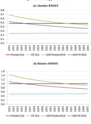
We implement 1-year recursive forecasting procedures stated in Section 3.2. As Kholodilin et al. (2008), we also calculate total RMSFE for all years at each forecasting horizon and relative RMSFE which is the ratio of total RMSFEs under the above three estimation methods over that under the benchmark (pooled OLS) forecast at each forecasting horizon. The former measures accuracy of forecasting. The latter measures the gains in accuracy compared with the benchmark case – the lower the relative RMSFE, the higher gains compared to simple pooled OLS estimation.

20

As can be seen in Figure 6(a), there is only a trivial increase in total RMSFE for the benchmark estimation, indicating that that forecast performance under pooled OLS would not deteriorate in the longer-term and is even better than spatial model set-up in the short run. The OLS for fixed-effects panel model produces lower total RMSFEs than those of the benchmark forecasting regardless of forecasting horizons, possibly because of the inclusion of statistically significant and substantial provincial fixed effects. When considering spatial dependence, both pooled and fixed-effects models yield higher total RMSFE in short forecasting horizon, but they perform better in the longer term, as indicated by lower total RMSFE than that of the benchmark after 2025. Spatial fixed-effects model is better than the pooled one, which again may be a result of inclusion of unignorable provincial fixed effects. Moreover, the gain in using SAR-FE, which is measured by the relative RMSFE in Figure 6(b), also becomes increasingly large in the longer term as its total RMSFE decreases and the difference in relative RMSFEs between SAR-FE and the benchmark case is increasingly wider after 2015. If this trend continued, it could be expected that SAR-FE-MLE would generate an even lower total as well as relative RMSFE compared with OLS estimation with fixed-effects in the long term after 2031. In general, our model fits the findings in the existing literature that taking spatial dependence into account improves forecast performance (e.g., Baltagi et al., 2014; Kholodilin et al., 2008). Together with significant spatial dependence found in Tables 3-4, we select the results of SAR-FE-MLE as our preferred forecasts instead of the OLS forecasts with fixed effects.

[Figure 6]

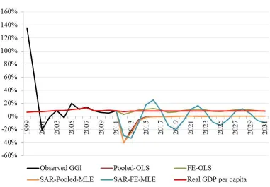
2001, the national green growth rate became stable around 8% until 2011, which is very close to the annual growth rate of GDP per capita. In the out-of-sample forecasts, as shown in Figure 7, OLS with fixed effects generates continuous stable green growth around the economic growth. In contrast, growth rates forecasted by two pooled estimations (OLS without spatial dependence and MLE with spatial dependence) would drop in the first three years until 2014 and then, quickly converge to zero. Our preferred forecasts under SAR-FE-MLE also predict a cyclical pattern around zero with smaller volatilities in growth rates in longer horizon. And in most of time, forecasted green growth rates are lower than projected economic growth, which is 8% according to the World Bank.

[Figure 7]

We also draw China’s prospect of green development in Figure 8. Consistent with Figure 7, only OLS estimation with fixed effects forecasts sustained green growth, which seems to synchronize with economic growth in the long-term. However, as mentioned earlier, OLS with fixed effects but without spatial dependence is likely to suffer from omitted variable problem and therefore, cannot be given much credibility. In comparison, all other three forecasting models reveal decreases in the level of green development in the near future prior to 2015. Moreover, there appears to be a cap on China’s green growth in the long-term. The SAR-FE-MLE forecasts appear to be cyclical given fluctuating green growth rates, while the highest level in forecasting horizon is always below that in 2011. The average green growth rate in the next two decades would be -2.5%, which is in sharp contrast to 19.4% over the period 1998-2011. China faces potentially huge challenges if she is to step onto a green development pathway.

Consistent with our finding of insignificant differences in regional unobserved heterogeneity, our forecasts do not reveal distinct green growth across eastern, central and western China, either. As listed in Table 7, the level of green development in the East used to increase quickest prior to 2011, but would drop quickest as well among the three. Green growth rates would decline first in the near future (2012-2017) and then fluctuate and converge gradually to zero. There is an overall downward trend in average green growth rates for the country as well as three regions prior to 2025, while the average rate would rebound to a positive but tiny value afterwards.

[Table 7]

5. Conclusion

Reference

Altenburg, T., Schmitz, H. and Stamm, A. (2008) Breakthrough? China’s and India’s transition from production to innovation. World Development 36, 325-344. Anselin, L. (2007) Spatial econometrics. In: T. C. Mills and K. Patterson (eds)

Palgrave Handbook of Econometrics (New York: Palgrave MacMillan), 901-969.

Auffhammer, M., and Carson, R. T. (2008) Forecasting the path of China’s CO2 emissions using provincial level information. Journal of Environmental

Economics and Management 55, 229–247.

Baltagi, B. H., Fingleton, B. and Pirotte, A. (2014) Estimating and forecasting with a dynamic spatial panel data model. Oxford Bulletin of Economics and Statistics

76, 112-138.

Brajer, V., Mead, R. W. and Xiao, F. (2011) Searching for an environmental Kuznets curve in China’s air pollution. China Economic Review 22, 383-397.

Blundell, R. and Bond, S. (1998) Initial conditions and moment restrictions in dynamic panel data models. Journal of Econometrics 87, 115–143.

Caselli, F., Esquivel, G. and Lefort, F. (1996) Reopening the convergence debate: A new look at cross-country growth empirics. Journal of Economic Growth 1, 363-389.

Chen, S. (2011) The abatement of carbon dioxide intensity in China: Factors decomposition and policy implications. The World Economy 34, 1148-1167. Chen, S. and Santos-Paulino, A. U. (2013) Energy consumption restricted

productivity re-estimates and industrial sustainability in post-reform China.

Chang, T., Hu, J., Chou, R. Y. and Sun, L. (2012) The sources of bank productivity growth in China during 2002-2009: A disaggregation view. Journal of Banking

and Finance 36, 1997-2006.

Cole, M. A., Elliott, R. J. R. and Zhang, J. (2011) Growth, foreign direct investment, and environment: Evidence from Chinese cities. Journal of Regional Science 51, 121-138.

de Vires, G., Erumban, A. A., Timmer, M. P., Voskoboynikov, I. and Wu, H. X. (2012) Deconstructing the BRICS: Structural transformation and aggregate productivity growth. Journal of Comparative Economics 40, 211-227.

Deininger, K., Jin, S. and Xia, F. (2012) Moving off the farm: Land institutions to facilitate structural transformation and agricultural productivity growth in China. World Bank Policy Research Working Paper No. 5949.

Dekle, R. and Vandenbroucke, G. (2012) A quantitative analysis of China’s structural transformation. Journal of Economic Dynamics and Control 36, 119-135.

Ding, S. and Knight, J. (2011) Why has China grown so fast? The role of physical and human capital formation. Oxford Bulletin of Economics and Statistics 73, 141-174.

Dollar, D. and Kraay, A. (2004) Trade, growth, and poverty. The Economic Journal

114, F22-F49.

Elhorst, J. P. (2010) Dynamic panels with endogenous interaction effects when T is Small. Regional Science and Urban Economics 40, 272–82.

Fei, L., Dong, S., Xue, L., Liang, Q. and Yang, W. (2011) Energy consumption-economic growth relationship and carbon dioxide emissions in China. Energy

Policy 39, 568-574.

Fingleton, B. and Le Gallo, J. (2008) Estimating spatial models with endogenous variables, a spatial lag and spatially dependent disturbances: Finite sample properties. Papers in Regional Science 87, 319-339.

Gibbons, S. and Overman, H. G. (2012) Mostly pointless spatial econometrics?

Journal of Regional Science 52, 172-191.

Hallegatte, S., Hela, G., Fay, M. and Treguer, D. (2011). From growth to green growth: A framework. World Bank Policy Research Working Paper 5872. Washington, DC: World Bank.

Hasan, I., Wachtel, P. and Zhou, M. (2009) Institutional development, financial deepening and economic growth: Evidence from China. Journal of Banking and

Finance 33, 157-170.

Holz, C. A. (2008) China’s economic growth 1978-2025: What we know today about China’s economic growth tomorrow. World Development 36, 1665-1691.

Holz, C. A. (2011) The unbalanced growth hypothesis and the role of the state: The case of China’s state-owned enterprises. Journal of Development Economics 96, 220-238.

Hossain, M. S. (2011) Panel estimation for CO2 emissions, energy consumption,

economic growth, trade openness and urbanization of newly industrialized countries. Energy Policy 39, 6991-6999.

Jia, R. (2013) Pollution for promotion. Mimeo. Available at: http://people.su.se/~rjia/papers/pollution_V20130420.pdf [accessed 12 October, 2013]

Jin, F. and Lee, L. (2013) Generalized spatial two stage least squares estimation of spatial autoregressive models with autoregressive disturbances in the presence of endogenous regressor and many instruments. Econometrics 1, 71-114.

Kapoor, M., Kelejian, H. H. and Prucha, I. R. (2007) Panel data models with spatially correlated error components. Journal of Econometrics 140, 97-130.

Kelejian, H. H. and Prucha, I. R. (1998) A generalised spatial two-stage least squares procedure for estimating a spatial autoregressive model with autoregressive disturbances. Journal of Real Estate Finance and Economics 17, 99-121.

Kelejian, H. H. and Prucha, I. R. (1999) A generalized moments estimator for the autoregressive parameter in a spatial model. International Economic Review 40, 509–533.

Kelejian, H. H. and Prucha, I. R. (2004) Estimation of simultaneous systems of spatially interrelated cross sectional equations. Journal of Econometrics 118, 27-50.

Kholodilin, K. A., Siliverstovs, B. and Kooths, S. (2008) A dynamic panel data approach to the forecasting of the GDP of German Länder. Spatial Economic

Analysis 3, 195-207.

Knight, J. and Ding, S. (2012) The role of structural change: Trade, ownership, industry. In: John Knight and Sai Ding (eds.): China’s Remarkable Economic Growth. Oxford University Press.

Kozul-Wright, R. and Fortunato, P. (2012) International trade and carbon emissions.

Lee, L. and Yu, J. (2010a) Estimation of spatial autoregressive panel data models with fixed effects. Journal of Econometrics 154, 165-185.

Lee, L. and Yu, J. (2010b) Efficient GMM estimation of spatial dynamic panel data models with fixed effects.

LeSage, J. P. and Pace, R. K. (2009) Introduction to spatial econometrics. Boca Raton, FL: CRC Press Taylor & Francis Group.

Lewis, J. I. (2010) The evolving role of carbon finance in promoting renewable energy development in China. Energy Policy 38, 2875-2886.

Lo, A. Y. (2013) Carbon trading in a socialist market economy: Can China make a difference? Ecological Economics 87, 72-74.

Managi, S., Hibiki, A. and Tsurumi, T. (2009) Does trade openness improve environmental quality? Journal of Environmental Economics and Management

58, 346-363.

Munro, N. (2013) Profiling the victims: public awareness of pollution-related harm in

China. Journal of Contemporary China, forthcoming, doi:

10.1080/10670564.2013.832532.

OECD (2011) Towards green growth: Monitoring progress. OECD, Paris.

Plümper, T. and Neumayer, E. (2010) Model specification in the analysis of spatial dependence. European Journal of Political Science 49, 418-442.

Rodrik, D. (2006) What’s so special about China’s exports? China & World Economy

14, 1-19.

Roodman, D. (2009) A note on the theme of too many instruments. Oxford Bulletin of

Su, F., Tao, R., Xi, L. and Li, M. (2012) Local officials’ incentives and China’s economic growth: Tournament thesis reexamined and alternative explanatory framework. China & World Economy 20, 1-18.

Toman, M. (2012). Green growth: An exploratory review. World Bank Policy Research Working Paper 6067. Washington, DC: World Bank.

Wang, A. L. (2013) The search for sustainable legitimacy: Environmental law and bureaucracy in China. Harvard Environmental Law Review 37, 365-440.

Wang, T. and Watson, J. (2010) Scenario analysis of China’s emissions pathways in the 21st century for low carbon transition. Energy Policy 38, 3537-3546.

Wang, S. S., Zhou, D. Q., Zhou, P. and Wang, Q. W. (2011) CO2 emissions, energy consumption and economic growth in China: A panel data analysis. Energy

Policy 39, 4870-4875.

Xue, B., Chen, X., Geng, Y., Guo, X., Lu, C., Zhang, Z. and Lu, C. (2010) Survey of officials’ awareness on circular economy development in China: Based on municipal and county level. Resources, Conservation and Recycling 54, 1296-1302.

Yanikkaya, H. (2003) Trade openness and economic growth: A cross-country empirical investigation. Journal of Development Economics 72, 57-89.

You, J. (2013) China’s challenge for decarbonized growth: Forecasts from energy demand models. Journal of Policy Modeling 35(4): 652-668.

Zheng, J., Bigsten, A. and Hu, A. (2009) Can China’s growth be sustained? A productivity perspective. World Development 37, 874-888.

Zheng, S., Kahn, M. E., Sun, W. and Luo, D. (2013) Incentives for China’s urban mayors to mitigate pollution externalities: The role of the central government and public environmentalism. Regional Science and Urban Economics, doi: http://dx.doi.org/10.1016/j.regsciurbeco.2013.09.003

Zhu, X. (2012) Understanding China’s growth: Past, present, and future. Journal of

Figure 1 Components of green growth

Source: Adopted Figure 1 on p. 17 in OECD (2011).

Figure 2 Cumulative distribution of green growth rates (1998-2011)

0 .2 .4 .6 .8 1

C

u

m

u

la

ti

v

e

pr

o

b

ab

ilit

y

-1 -.5 0 .5 1

Green growth rate

Figure 3 Relation between the green growth rate and real GDP per capita beijing tianjin hebei shanxi inner_monglia liaoning jilin_heilongjiang shanghai jiangsu zhejiang anhui fujian jiangxi shandong henan hubei hunan guangdong guangxi hainan chongqing sichuan guizhou yunnan shaanxi gansu ningxia xinjiang -. 8 -. 6 -. 4 -. 2 0 G ree n gro w th r a te

0 10,000 20,000 30,000

GDP per capita (yuan in 2011 prices)

LOWESS smoothing of green growth rates Green growth rate

(a) 1998 beijing tianjin hebei shanxi inner_monglia liaoning jilin heilongjiang shanghai jiangsu zhejiang anhui fujian jiangxi shandong henan hubei hunan guangdong guangxi hainan chongqing sichuan guizhou yunnan shaanxi gansu qinghai ningxia xinjiang -. 1 0 .1 .2 G ree n gro w th r a te

20,000 40,000 60,000 80,000 100,000

GDP per capita (yuan in 2011 prices)

LOWESS smoothing of green growth rates Green growth rate

Figure 4 Estimated province fixed effects

Note: East, middle and west provinces are labeled by blue, orange and grey bars, respectively. The classification of three regions follows the NBS criteria.

Figure 5 Growth rates of GDP per capita and productivity of abiotic and biotic

Figure 6 Forecasting performance

(a) Absolute RMSFE

Figure 8 China’s green growth vs. economic growth

Table 1 Components of China’s provincial green growth indexa

Category Indicator Definition Data source and/or construction procedures

1: The socio-economic context and characteristics of growth

Real GDP Real GDP index (1997=100) Authors’ calculation based on GDP and CPI data from China Statistical Yearbooks

published by the NBS.

Population density Inhabitants per km2 Authors’ calculation based on population and areas data from China Statistical Yearbooks published by the NBS.

2: Environmental and resource productivity

Production-based CO2 productivity

Real yuan per kg of CO2 We follow Auffhammer and Carson’s (2008) method to estimate provincial CO2

emissions. Specifically, we regress the national CO2 emissions on the national

industrial waste gas and the time control variables over the period 1997-2011 and then, use the estimated coefficients and the observed provincial industrial waste gas to calculate provincial CO2 emissions. To keep consistency with the OECD Green

Growth Database, we draw data on China’s national CO2 emissions from IEA

Energy Database. National and provincial industrial waste gas emissions are collected from China Statistical Yearbooks.

Energy productivity Real GDP (in yuan) per ton of

standard coal equivalent of total primary energy supply

Authors’ calculation based on data of total primary energy supply from China Energy Statistical Yearbooks and provincial statistical yearbooks, and provincial GDP, population and CPI data from China Statistical Yearbooks.

Energy intensity Ton of standard coal equivalent of total primary energy supply per capita

Renewable energy

supply

Share of renewable energy supply in total primary energy supply

Authors’ calculation based on primary energy supply as obtained above and renewable energy supply. The latter comes from China Energy Statistical

Yearbooks and provincial statistical yearbooks. Note that our provincial ‘renewable energy supply’ includes only electricity generated by hydro power, and nuclear and wind power due to data availability, while the OECD definition further includes geothermal, solar, tide and combustible renewables and waste compromises biomass.

Non-energy material

consumption

Non-energy domestic material consumption (DMC) index (1997=100)

Authors’ calculation. According to OECD, non-energy DMC equals biotic materials (to be explained below) plus abiotic materials (to be explained below) plus

construction materials (to be explained below). All data are measured in weight (kg) rather than monetary terms. The value in 1997 is set as 100, and all subsequent values are compared to it.

non-energy DMC

Biotic material

productivity

Real GDP (in yuan) per kg of biotic material DMC

Authors’ calculation. This indicator is measured as the real GDP in China Statistical Yearbooks divided by biotic material DMC. According to Eurostat and OECD, the biotic material DMC equals agricultural domestic production plus agricultural import minus agricultural export. All data are measured in weight (kg). Agricultural domestic production is measured as the sum of products of farm, forest, and fishing. Specifically, we incorporate rice, wheat, corn, beans, tubers, cotton, oil-bearing crops (peanuts, rapeseeds and sesame), fibre crops, sugarcane, beetroots, tobacco, silkworm cocoons, tea, fruits (apples, citrus, pears, grapes and bananas), meat (poultry, pork, beef and mutton), milk, eggs, honey, sheep wool, goat wool, cashmere, rubber, turpentine, raw lacquer, Tung-oil seeds, tea-oil seeds, walnuts, logs, sawn timber, and aquatic products (seawater and freshwater aquatic products). Relevant data come from China Statistical Yearbooks published by the NBS and China Agricultural Statistical Yearbooks published by the Ministry of Agriculture. There are no data on provincial agricultural imports and exports. According to OECD, import and export include both raw materials and semi-products, in order to reflect comprehensively material flows. We estimate provincial agricultural import and export in the spirit of Auffhammer and Carson (2008) again. Specifically, we first calculate national agricultural import, which is the sum of cereals and cereal powder, soybeans, rice, corn, wheat, cotton, vegetable oil, sugar, feed, wool, rubber, logs, sawn timber, pulp and resin, and national agricultural export, which is the sum of cereals and cereal powder, soybeans, rice, corn, cotton, ramie, raw silk, willow-, bamboo- and cane-weaving products, vegetable oil, aldose, walnut seeds, peanuts and peanut seeds, pine nuts, hazelnuts, dried beans, vegetables, meat (poultry, pork, beef and rabbit), milk, eggs, honey, tobacco, tea, fruits (apples and citrus), aquatic products, cashmere, cony wool, paper, turpentine and resin. Relevant data come from China Statistical Yearbooks published by the NBS and China Customs

Statistics Yearbooks published by the General Administration of Customs of China. Then, we regress national agricultural import and export on national total import and export volumes and time control variables, respectively. We finally calculate provincial agricultural import and export by using the estimated coefficients and observed provincial total import and export volumes, respectively. Real national and provincial import and export volumes are authors’ calculations based on relevant nominal and price data from China Statistical Yearbooks.

abiotic material DMC equals domestic metal production plus domestic non-metallic industrial minerals and construction materials plus imported metal and non-metallic minerals and construction materials minus those exported. All data are measured in weight (kg). Domestic metal production is the sum of pig iron, crude steel, rolled steel and 10 kinds of nonferrous metal. Domestic non-metallic industrial minerals are the sum of salt, plastics and sulphur. Domestic non-metallic construction materials are the sum of common clays and glass. Relevant data come from China Steel Statistical Yearbooks, China Nonferrous Metal Statistical Yearbooks, China Construction Statistical Yearbooks, and China Statistical Yearbooks of Chemical Industry. There are no data on provincial import and export of abiotic materials. According to OECD, import and export include both raw materials and semi-products, in order to reflect comprehensively material flows. We also estimate provincial import and export in the spirit of Auffhammer and Carson (2008).

Specifically, we first calculate national import of abiotic materials, which is the sum of urea, copper and aluminium and their alloy, manganese, and ore sand of iron, copper, manganese and chromium. We also calculate national export of abiotic materials, which is the sum of which is the sum of glass, clay, pig iron, steel, steel billet and rough forging products of steel, ferrosilicon, copper, steel- and copper-made fasteners, talc, ceramics, ore sand of copper, plastics, sulphur, graphite, fluorite, and aluminium, manganese,

Yearbooks. Then, we regress national import and export of abiotic materials on national total import and export volumes and time control variables, respectively. We finally calculate provincial import and export of abiotic materials by using the estimated coefficients and observed provincial total import and export volumes, respectively. Real national and provincial import and export volumes are authors’ calculations based on relevant nominal and price data from China Statistical Yearbooks.

3: Monitoring the natural asset baseb

Available water resources

m3 of total available water supply per capita

Authors’ calculation based on data of total water supply and population from China Statistical Yearbooks.

Total water

abstraction

Tons of total tap water supply per capita

Authors’ calculation based on data of total tap water supply and population from China Statistical Yearbooks.

4: Monitoring the environmental quality of lifec

Urban: Sewerage density

Urban: Length of sewerage pipelines (km) per km2 of urban areas