Modelling and Bayesian Inference of the Abakaliki
Smallpox Data: Supplementary Material
We describe (i) for the likelihood, how to integrate out the unknown protection statuses of individuals outside the compound; (ii) the details of the MCMC algorithm. For ease of reference we start by recalling the notation used.
1
Notation
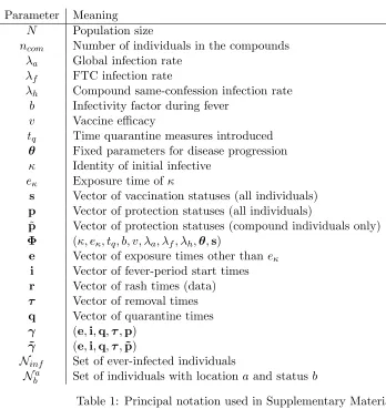
The principal notation used is listed in Table 1, most of which is also used in the main manuscript. We also extend the notation of the main manuscript for sets of individuals; specifically,Na
b is used to denote a set of individuals with characteristicsa and b, wherea
denotes location (such asOC, meaning outside the compound) andbdenotes status such as FTC or n-FTC (i.e. not FTC), sus (initially susceptible), inf (ever infected) or n-inf (never infected). Note that ‘initially susceptible’ can mean either ‘not vaccinated’ or ‘vaccinated, but not protected’.
2
Transformation of the Likelihood
We now explain how to write the likelihood in a form that does not include the protection statuses for individuals outside of the compounds. In section 2.1 we will show that
π(r,γ|Φ) =π(r,˜γ, x, y|Φ), (1)
where instead of separate protection statuses for each outside individual, we only require quantities xand y where
x = Number of FTC, vaccinated, unprotected but never
infected individuals outside the compounds
y = Number of non-FTC, vaccinated, unprotected but
Parameter Meaning N Population size
ncom Number of individuals in the compounds
λa Global infection rate
λf FTC infection rate
λh Compound same-confession infection rate
b Infectivity factor during fever v Vaccine efficacy
tq Time quarantine measures introduced
θ Fixed parameters for disease progression κ Identity of initial infective
eκ Exposure time ofκ
s Vector of vaccination statuses (all individuals) p Vector of protection statuses (all individuals) ˜
p Vector of protection statuses (compound individuals only) Φ (κ, eκ, tq, b, v, λa, λf, λh,θ,s)
e Vector of exposure times other than eκ
i Vector of fever-period start times r Vector of rash times (data) τ Vector of removal times q Vector of quarantine times γ (e,i,q,τ,p)
˜
γ (e,i,q,τ,p)˜
Ninf Set of ever-infected individuals
Na
[image:2.612.74.422.212.581.2]b Set of individuals with location aand statusb
and where
˜
γ = (e,i,q,τ,˜p)
where p˜ = (p0, p1, ..., pncom−1). Thus γ˜ is the same as γ but with protection statuses for individuals inside the compounds only.
Given (1), x and y can then be integrated out to yield a likelihood which is computa-tionally much faster to calculate. First note that
π(r,γ˜, x, y|Φ) =π(r,˜γ|x, y,Φ)π(x, y|Φ)
and hence
π(Φ,γ˜, x, y|r) = π(r,γ˜|x, y,Φ)π(x, y|Φ)π(Φ)
π(r) .
Integrating out x and y, which is equivalent to summing in this case since they take discrete values, we obtain the new target density
π(Φ,˜γ|r) =X
x,y
π(Φ,˜γ, x, y|r) = π(Φ) π(r)
X
x,y
π(r,˜γ|x, y,Φ)π(x, y|Φ).
2.1 Derivation of equation (1)
First, note that bothxandy are determined by the data, the vaccination status of individ-uals outside the compound, and the protection status of individindivid-uals outside the compound. Since only the latter is unknown, we may think of x and y as functions of p, or more pre-cisely those elements ofp that correspond to vaccinated individuals outside the compound. In particular, summation over all values of x and y is equivalent to summation over such elements of p.
Recall that Λ(t) denotes the total infectious pressure acting on all susceptibles at time t, and that we have
π(r,γ|Φ) =
Y
j∈Ninf
Λj(ej−)
×e
−RT eκΛ(t)dt
× Y
j∈Ninf
fI(ij−ej)fF(rj−ij)fR(τj−rj)fQ(qj −max(rj, tq))
×v
N−1
P
r=0 prsr
(1−v)
N−1
P
r=0
(1−pr)sr
. (2)
We may write Λ(t) = ΛOC(t) + ΛCN(t) + ΛCC(t), where (i) ΛOC(t) is the pressure on
individuals outside the compounds; (ii) ΛCN(t) is the pressure on those inside the
infected. Then the only terms in (2) with unknown protection statuses for outside individ-uals are ΛOC(t) and the terms involving v. We now expand the likelihood of the protection
status, according to whether each individual is inside/outside and by whether they do/do not become infected, as follows:
v
N
P
r=0 prsr
(1−v)
N
P
r=0
(1−pr)sr
=v
ncom−1
P
r=0 prsr
(1−v)
ncom−1
P
r=0
(1−pr)sr
×v
N
P
r=ncom prsr
(1−v)
N
P
r=ncom r∈Ninf
(1−pr)sr
×(1−v)
N
P
r=ncom r∈Nn−inf
(1−pr)sr
.
The terms corresponding to individuals inside the compounds do not depend on x and y, and neither does the term concerning outside infectives, since their protection status is known. Thus the part of the likelihood dependent on x and y, which are determined by p as previously explained, is
Lx,y(p) = e−
RT
eκΛOC(t)dtv N
P
r=ncom prsr
(1−v)
N
P
r=ncom r∈Nn−inf
(1−pr)sr
. (3)
The integral of ΛOC is the sum over all infectivesjof the pressure fromjto any given FTC
or non-FTC individual outside of the compounds (throughout all time (eκ, T)), summed
over all the initially susceptible FTC and non-FTC individuals. Thus,
e−
RT
eκΛOC(t)dt = exp
− X
j∈Ninf
X
k∈Noc sus
Ψjk
(4)
with Ψjk = total infectious pressure fromjto susceptiblekduring the time interval (eκ, T).
We now expand the right-hand side of (4) according to whether susceptibles become infected or not, and whether they are FTC or not, yielding
exp− X
j∈Ninf
X
k∈Noc sus
Ψjk
= exp − X
j∈Ninf
X
k∈Noc inf
Ψjk +
X
k∈Noc n−inf
Ψjk
!
= exp − X
j∈Ninf
X
k∈Noc inf,F T C
Ψjk +
X
k∈Noc inf,n−F T C
Ψjk
+ X
k∈Noc n−inf,F T C
Ψjk +
X
k∈Noc
n−inf,n−F T C
Ψjk
!
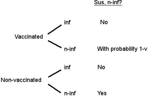
Figure 1: Tree diagram for protection status of individuals outside the compounds.
Recall that the data only tell us if individuals are vaccinated, not whether they are protected. Of the four Ψjk values in equation (5), the numbers of initially susceptible FTC and
non-FTC individuals outside that do become infective are known, but not the number of initial susceptibles that are never infected. Figure 1 displays how individuals can be in the latter two categories.
So, the total number of initially susceptible, never infected individuals outside the com-pounds is given by
| Nnoc−inf| =aocn−inf,F T C+aocn−inf,n−F T C+x+y
where aocn−inf,F T C is the known number of non-vaccinated, never infective FTC individ-uals outside the compounds and aocn−inf,n−F T C is the corresponding number of non-FTC individuals. Using this and (5), (3) becomes
Lx,y(p) = exp
− X
j∈Ninf
X
k∈Noc inf,F T C
Ψjk +
X
k∈Noc inf,n−F T C
Ψjk
+χF(j)×(aocn−inf,F T C+x) +χN F(j)×(aocn−inf,n−F T C+y)
×v
N
P
r=ncom prsr
(1−v)
N
P
r=ncom r∈Nn−inf
(1−pr)sr
where
χF(j) = b(rj−ij) + (min(qj, τj)−rj)
×
( λa
N−1 +
λf
n−1 iffj = FTC
λa+λf
N−1 otherwise and
χN F(j) = b(rj−ij) + (min(qj, τj)−rj)
×
( λa
N−1 iffj = FTC
λa+λf
N−1 otherwise
represent respectively the contribution from infective j to a never infected FTC and non-FTC susceptible outside the compounds over all time (eκ, T), this contribution being equal
for all susceptiblesk.
Considering the protection status likelihood parts of equation (6), note that
(1−v)
N
P
r=ncom r∈Nn−inf
(1−pr)sr
= (1−v)x+y,
since the sum is equal to the number of vaccinated but unprotected individuals outside who do not become infected, and hence
v
N
P
r=ncom prsr
=vbocn−inf−x−y,
wherebocn−inf is the number of never-infected vaccinated individuals outside the compounds. Splitting up the terms involving x and y, equation (6) can be written in the form
Lx,y(p) =
exp
− X
j∈Ninf
X
k∈Noc inf,F T C
Ψjk+
X
k∈Noc inf,n−F T C
Ψjk+aocn−inf,F T CχF(j) +aocn−inf,n−F T CχN F(j)
!
×exp − X
j∈Ninf
χF(j)×x
!
×(1−v)xvbocn−inf,F T C−x
×exp − X
j∈Ninf
χN F(j)×y
!
×(1−v)yvbocn−inf,n−F T C−y (7)
2.2 Removing x and y
We now sum (7) over x and y. Recall that this is equivalent to summing Lx,y(p) over all
possible values of the elements ofprelating to vaccinated individuals outside the compound. For fixedx and y, write p(x, y) for a typical vectorp that yields x and y. First note that the number of possible vectors p(x, y) is
bocn−inf,F T C x
bocn−inf,n−F T C y
,
where bocn−inf,F T C and bocn−inf,n−F T C are respectively the (known) number of vaccinated, not-infected FTC and non FTC individuals outside the compounds. We may thus write
Lx,y=
X
p(x,y)
Lx,y(p) =
bocn−inf,F T C x
bocn−inf,n−F T C y
Lx,y(p),
which in combination with (7) means that the required sums (over x and y, which can be separated from each other) are of the form
b
X
x=0
b x
e−αx(1−v)xvb−x = ((1−v)e−α+v)b.
WritingL=P
x,yLx,y,χF =
P
j∈Ninf
χF(j) and χN F = P j∈Ninf
χN F(j) we thus obtain
L = exp− X
j∈Ninf
X
k∈Noc inf,F T C
Ψjk+
X
k∈Noc inf,n−F T C
Ψjk
− aocn−inf,F T CχF −aocn−inf,n−F T CχN F
×(1−v)e−χF +vb
oc
n−inf,F T C
(1−v)e−χN F +vb
oc
n−inf,n−F T C
. (8)
algo-rithm we work with log-likelihood, so taking logs gives an overall log likelihood of
log(π(r,˜γ|Φ)) = log
Y
j∈Ninf j6=κ
Λj(ej−)
−
Z T
eκ
(ΛCN(t)−ΛCC(t))dt−
X
j∈Ninf
X
k∈Noc inf
Ψjk
−aocn−inf,F T CχF −aocn−inf,n−F T CχN F
+bocn−inf,F T Clog v+ (1−v)e−χF+boc
n−inf,n−F T Clog v+ (1−v)e−χN F
+ log
Y
j∈Ninf
fI(ij−ej)fF(rj−ij)fR(τj−rj)fQ(qj −max(rj, tq))
+
ncom−1
X
r=0
sr prlog(v) + (1−pr) log(1−v)
+
N−1
X
r=ncom r∈Ninf
srlog(1−v).
3
MCMC
Here we give details of the MCMC algorithm.
3.1 Unknown vaccination statuses in MCMC algorithm
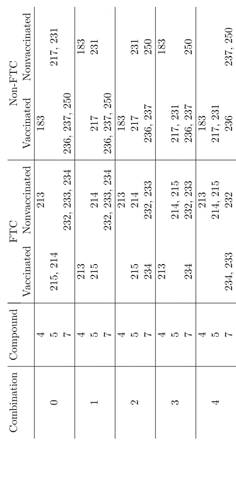
Although the total number of vaccinated individuals within the Abakaliki compounds is known, we do not have complete information on the composition of compound individuals with respect to vaccination status and FTC membership. Table 2 shows 5 potential con-figurations of the 12 individuals with unknown details. This means that all the elements ofs (the vector of vaccination statuses) are assumed known, with 12 exceptions, which can take 5 possible configurations. A described below in the MCMC algorithm, updates to s involve potentially changing the configuration from the 5 that are possible, while all other elements of sare unchanged.
3.2 Full conditional Distributions
Here we give, up to proportionality, the full conditional distributions for the parameters that will be updated in the MCMC algorithm. Although in principle we could update all parameters individually using a Metropolis-Hastings step involving the full likelihood, algorithm efficiency is increased if we only include those parts of the likelihood that can change during a particular update.
The parameters to be updated are tq, λa, λf, λh, v, b, ˜p, s and the exposure, fever,
generic unknown constant (arising from the fact that we generally only know full conditional distributions up to proportionality).
log(π(tq|r,θ,γ˜, κ, b, v, λa, λf, λh, eκ,s)) +c=
log
Y
j∈Ninf
Λj(ej−)
− Z T
eκ
(ΛCN(t) + ΛCC(t))dt−log(L) + log(π(tq)).
log(π(b|r,θ,˜γ, κ, tq, v, λa, λf, λh, eκ,s)) +c=
log
Y
j∈Ninf
Λj(ej−)
− Z T
eκ
(ΛCN(t) + ΛCC(t))dt−log(L) + log(π(b)).
log(π(v|r,θ,γ˜, κ, tq, b, λa, λf, λh, eκ,s)) +c=
−log(L) +
ncom−1
X
r=0
prsrlog(v) + ncom−1
X
r=0
(1−pr)srlog(1−v)
+
N−1
X
r=ncom r∈Nn−inf
(1−pr)srlog(1−v) + log(π(v)).
log(π(λa|r,θ,γ˜, κ, tq, v, b, λf, λh, eκ,s)) +c=
log
Y
j∈Ninf
Λj(ej−)
− Z T
eκ
(ΛCN(t) + ΛCC(t))dt−log(L) + log(π(λa)).
log(π(λf|r,θ,˜γ, κ, tq, v, b, λa, λh, eκ,s)) +c=
log
Y
j∈Ninf
Λj(ej−)
− Z T
eκ
(ΛCN(t) + ΛCC(t))dt−log(L) + log(π(λf)).
log(π(λh|r,θ,γ˜, κ, tq, v, b, λf, λa, eκ,s)) +c=
log
Y
j∈Ninf
Λj(ej−)
− Z T
eκ
For any i= 0,1, . . . , ncom−1, defining ˜pi∗ = (p0, p1, ..., pi−1, pi+1, ..., pncom−1),
log(π(˜pi|r,Φ,e,i,q,τ,p˜∗i)) +c=
−
Z T
eκ
ΛCN(t)dt+pilog(v) + (1−pi) log(1−v).
log(π(s|r,θ,˜γ, κ, tq, v, b, λa, λh, eκ)) +c=
−
Z T
eκ
ΛCN(t)dt+ ncom−1
X
r=0
prsrlog(v) + ncom−1
X
r=0
(1−pr)srlog(1−v)
+
N−1
X
r=ncom r∈Nn−inf
(1−pr)srlog(1−v).
Finally, fori= 0,1, ..., N−1 whereiis infective, defininge∗i = (e0, e1, ..., ei−1, ei+1, ..., eN−1) and similarly defining i∗i,q∗i and τ∗i,
log(π(ei|r,Φ,e∗i,i,q,τ,p)) +˜ c=
log
Y
j∈Ninf
Λj(ej−)
− Z T
eκ
(ΛCN(t) + ΛCC(t))dt−log(L).
log(π(ii|r,Φ,e,ii∗,q,τ,p)) +˜ c=
log
Y
j∈Ninf
Λj(ej−)
− Z T
eκ
(ΛCN(t) + ΛCC(t))dt−log(L).
log(π(qi|r,Φ,e,i,q∗i,τ,˜p)) +c=
log
Y
j∈Ninf
Λj(ej−)
− Z T
eκ
(ΛCN(t) + ΛCC(t))dt−log(L).
log(π(τi|r,Φ,e,i,q,τ∗i,˜p)) +c=
log
Y
j∈Ninf
Λj(ej−)
− Z T
eκ
3.3 MCMC Algorithm
The MCMC algorithm consists of individual Metropolis-Hastings updates for all of the required parameters. For a generic parameter α the update consists of a proposed new value α∗ drawn from proposal density (or mass function)q(α∗|α), which is then accepted with probability
min
π(α∗)q(α|α∗) π(α)q(α∗|α),1
,
whereπ(α∗) andπ(α) denote the full conditional density (or mass function) forαevaluated at the proposed and current value, respectively. In most cases below, the proposal density q is symmetric in the sense that q(α|α∗) =q(α∗|α), which simplifies the computations.
For tq,λa,λf,λh,v, andb, we use a Gaussian proposal distribution with pre-specified
variance, centered on the current parameter value. Proposed values outside the possible set for each parameter are immediately rejected (for example, all the infection rates must be positive, 0≤v ≤1, etc.) Note that if such a rejection occurs, no further proposal attempt is made. The acceptance probability is calculated using the full conditional distributions listed above.
Protection status updates (i.e. updates to p) are achieved by first randomly selecting a˜ fixed number (e.g. 5 or 10) of compound individuals among those who were vaccinated but never infected, and proposing to change the protection status of each selected individual.
Updates to s are similar: a proposed new value is chosen uniformly at random from one of the five possible configurations of the 12 individuals whose vaccination status is uncertain, as shown in Table 2. Following this, all of the individuals among the 12 who are now proposed to be vaccinated are, independently with probability v, proposed to be protected, while those proposed to be unvaccinated are proposed to be unprotected.
Finally, updates to the event times are carried out in pairs, the reason being that we expect these quantities to be correlated. Specifically, an individual is chosen uniformly at random from the set of infected individuals, and proposed new exposure and fever times are simulated from the distributions assumed in the model. These are then accepted or rejected as usual. Following this, a pair of removal and quarantine times are proposed for the same individual, regardless of whether or not the exposure and fever times were changed. In practice we repeat the entire event-time-updating procedure a number of times (e.g. 5) within each full MCMC iteration in order to improve the overall algorithm mixing.