Diffusion driven oscillations in gene regulatory networks

(1)

Di

ff

usion Driven Oscillations in Gene Regulatory Networks

Cicely K Macnamara∗_{, Mark AJ Chaplain}

School of Mathematics and Statistics, Mathematical Institute, University of St Andrews, United Kingdom, KY16 9SS

Abstract

Gene regulatory networks (GRNs) play an important role in maintaining cellular function by correctly timing key pro-cesses such as cell division and apoptosis. GRNs are known to contain similar structural components, which describe how genes and proteins within a network interact - typically by feedback. In many GRNs, proteins bind to gene-sites in the nucleus thereby altering the transcription rate. If the binding reduces the transcription rate there is a negative feedback leading to oscillatory behaviour in mRNA and protein levels, both spatially (e.g. by observing fluorescently labelled molecules in single cells) and temporally (e.g. by observing protein/mRNA levels over time). Mathematical modelling of GRNs has focussed on such oscillatory behaviour. Recent computational modelling has demonstrated that spatial movement of the molecules is a vital component of GRNs, while it has been proved rigorously that the diffusion coefficient of the protein/mRNA acts as a bifurcation parameter and gives rise to a Hopf-bifurcation. In this paper we consider the spatial aspect further by considering the specific location of gene and protein production, showing that there is an optimum range for the distance between an mRNA gene-site and a protein production site in order to achieve oscillations. We first present a model of a well-known GRN, the Hes1 system, and then extend the approach to examine spatio-temporal models of synthetic GRNs e.g. n-gene repressilator and activator-repressor systems. By incorporating the idea of production sites into such models we show that the spatial component is vital to fully understand GRN dynamics.

Keywords: Hes1 protein, synthetic networks, repressilators, activator-repressor systems, spatial modelling

1. Introduction 1

A gene regulatory network (GRN) can be defined as

2

a collection of DNA segments in a cell which interact

3

with each other indirectly through their RNA and

4

protein products. GRNs lie at the heart of intracellular

5

signal transduction and indirectly control many

import-6

ant cellular functions such as cell division, apoptosis

7

and adhesion. One key class of GRNs is a group of

pro-8

teins called transcription factors. As the name suggests,

9

in response to a range of signals, transcription factors

10

change the transcription rate of genes, allowing cells

11

to alter the levels of proteins they require at any given

12

time. A GRN is said to contain a negative feedback

13

loop if a gene product inhibits its own production either

14

∗_{Corresponding author.}

Phone:+44 (0)1334 463723

Email addresses:ckm@st-andrews.ac.uk(Cicely K Macnamara),majc@st-andrews.ac.uk(Mark AJ Chaplain)

directly or indirectly, and similarly, is said to contain

15

a positive feedback loop if a gene product enhances

16

its own production either directly or indirectly. In

17

particular, the modification of the transcription of genes

18

by proteins (transcription factors) through negative

19

feedback (down-regulation) is an important component

20

of many gene networks, and such negative feedback

21

systems are known to exhibit oscillations in the levels

22

of the molecules involved. Negative feedback loops

23

are commonly found in diverse biological processes

24

including inflammation, meiosis, apoptosis and the heat

25

shock response (Lahav et al., 2004), where the

oscillat-26

ory expression is of particular importance. In addition

27

to their natural occurrence, GRNs have also become

28

an important focus in the emerging field of synthetic

29

biology. Since the pioneering work of Becskei and

30

Serrano (2000) and Elowitz and Leibler (2000), there

31

has been a great deal of interest in synthetic GRNs, both

32

from a practical, experimental viewpoint (Balagadde

33

et al., 2008; Chen et al., 2012; Yordanov et al., 2014)

(2)

and from a theoretical, modelling viewpoint (Purcell

35

et al., 2010; O’Brien et al., 2012).

36

37

Mathematical modelling of GRNs can be traced

38

back 50 years to the seminal paper of Goodwin (1965),

39

followed shortly after by the paper of Griffith (1968).

40

These papers proposed a generic “closed-loop” negative

41

feedback model for a simple mRNA-protein feedback

42

system (which we note is appropriate to model the

43

actual Hes1 protein system, Hirata et al. (2002)). The

44

models were restricted to purely temporal ODEs and

45

oscillatory behaviour was elusive. Mackey and Glass

46

(1977) introduced the idea of incorporating delays into

47

differential equations. Delay-differential equation

mod-48

els for GRNs have been studied extensively for the last

49

two decades, since the early work of Smolen, Baxter

50

and Byrne (e.g. Smolen et al., 1999, 2001, 2002). Of

51

particular interest here is Smolen et al. (1999) where the

52

relation between delays and macromolecular transport

53

was discussed. Specifically, their GRN model used a

54

delay to account for active transport of molecules and

55

showed that while such a model leads to oscillatory

56

behaviour, incorporating molecular diffusion supressed

57

oscillations. Other more recent models, including

58

models of the Hes1 system, the p53-Mdm2 system

59

and the NF-κB system, also showed that delays were

60

found to provoke oscillatory behaviour (Tiana et al.,

61

2002; Jensen et al., 2003; Lewis, 2003; Monk, 2003;

62

Bernard et al., 2006). Theoretical models of synthetic

63

GRNs (e.g. repressilators) have also been proposed and

64

studied (Purcell et al., 2010; O’Brien et al., 2012), while

65

interest in modelling bacterial operons by Mackey and

66

co-workers (Yildirim and Mackey, 2003; Hilbert et al.,

67

2011; Mackey et al., 2015) has added additional insight.

68

69

Early spatial models of theoretical intracellular

70

systems were pioneered in the 1970s by Glass and

71

co-workers (Glass and Kauffman, 1970; Shymko and

72

Glass, 1974) and again in the 1980s by Mahaffy and

73

co-workers (Busenberg and Mahaffy, 1985; Mahaffy,

74

1988; Mahaffy and Pao, 1984), where the focus was

75

on analysing generic systems with one-dimensional

76

models. ODE models were reconfigured to incorporate

77

a spatial dimension using reaction-diffusion PDEs and

78

steady states and stability were determined with

partic-79

ular attention paid to the geometry of the model. They

80

coined the term “spatial switching” to indicate how

81

the system geometry can lead to different dynamical

82

behaviour. This approach has recently been extended

83

by Naqib et al. (2012). Other spatial models have

84

focussed on the idea of modelling a cell using two (or

85

more) compartments, to account for different processes

86

which occur in the nucleus and cytoplasm (see, for

87

example, Sturrock et al., 2011, 2012); certain models

88

incorporate both compartments and delays (e.g. Momiji

89

and Monk, 2008). A two-dimensional spatial model

90

of molecular transport inside a cell was formulated by

91

Cangiani and Natalini (2010) and this general approach

92

was adopted by Sturrock et al. (2011) to formulate

93

and study a spatio-temporal model of the Hes1 GRN

94

considering diffusion of the protein and mRNA. This

95

model was then later extended to account for transport

96

across the nuclear membrane and directed transport

97

via microtubules (Sturrock et al., 2012). Other papers

98

adopting an explicitly spatial approach include those

99

of Szyma´nska et al. (2014), focussing on the role of

100

transport via the microtubules, and Clairambault and

101

co-workers (Dimitrio et al., 2013; Eliaˇs and

Clairam-102

bault, 2014; Eliaˇs et al., 2014a,b), focussing on the p53

103

system.

104

105

In this paper we focus on the spatial component,

106

by supposing that the different processes within a

107

given GRN occur at specific sites. This approach

108

removes the requirement to consider compartments

109

and instead localises mRNA and protein production.

110

The initial Hes1 model is an extension of the model of

111

Sturrock et al. (2011, 2012) and is inspired by the recent

112

result of Chaplain et al. (2015) where it was proved

113

rigorously that molecular diffusion causes oscillations.

114

We develop and analyse spatio-temporal mathematical

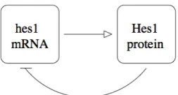
115

models for synthetic GRNs, focussing on the role of

116

diffusion and the spatial location of the gene sites and

117

protein production sites in generating and controlling

118

the oscillatory dynamics.

119

120

The paper is structured as follows. In Section 2

121

we discuss the results of the canonical GRN, the Hes1

122

system. In Sections 3 and 4 we develop models and

123

present simulation results for three different synthetic

124

GRNs, specifically repressilators and

activator-125

repressors. Discussions, conclusions and directions for

126

future work in this area are given in the final Section 5.

127

2. The Hes1 System 128

The Hes1 protein is a member of the family of

ba-129

sic helix-loop-helix (bHLH) transcription factors and

130

is known to repress the transcription of its own gene

131

through direct binding to regulatory sequences in the

132

Hes1 promoter (Hirata et al., 2002). For this reason,

133

it may be termed the canonical transcription factoror

134

canonical gene regulatory network. It is known that

135

periodically changing levels of Hes1 protein controls

(3)

embryonic development, specifically in correctly timed

137

somite segmentation (see, for example, Kageyama et al.,

138

2007). Mathematical modelling is particularly well

139

suited to the relatively simple Hes1 system, which is

140

controlled by way of a single negative feedback loop

141

between its mRNA and protein. Of particular interest

142

here is spatial modelling. Sturrock et al. (2011) showed

143

that a two compartment, nucleus-cytoplasm

reaction-144

diffusion model gives rise to oscillatory behaviour,

145

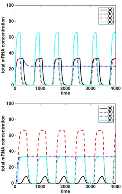
while Chaplain et al. (2015) rigorously proved that the

146

diffusion parameter controls whether or not the system

147

oscillates. Here we modify the model used by

Chap-148

lain et al. (2015) to incorporate sites at which the hes1

149

mRNA and Hes1 protein will be produced. For the

pur-150

poses of discussion we will refer to locations of mRNA

151

production as “gene-sites” and protein production as

152

“production sites”. We present results for a 1D

inter-153

val model, however they equally apply to models of the

154

system in other geometries, specifically 2D circular and

155

elliptical and 3D spherical, (more details can be found

156

in Appendix B). We consider the non-dimensional (see

157

2.1 for details of the non-dimensionalisation) form of

158

the 1D model to be:

159

∂m ∂t =D

∂2_m ∂x2 +

αm

1+phδ

ε

xm(x)−µm,

∂p ∂t =D

∂2_p

∂x2 +αpmδ

ε

xp(x)−µp,

(1)

wherem(x,t) and p(x,t) are the concentrations of hes1

160

mRNA and Hes1 protein, respectively. Initially (and for

161

simplicity) we assume that both mRNA and protein

dif-162

fuse through the cell with the same constant diffusion

163

coefficient, D, and are subject to degradation

(propor-164

tional to their concentrations) at the same rate,µ. The

165

protein is translated at a production site located at

po-166

sition xp, at a rate αp and proportional to the level of 167

mRNA. The presence of the protein then represses the

168

production of mRNA (modelled by a Hill function with

169

Hill coefficient h) which undergoes transcription at a

170

gene-site located at positionxm, at a rateαm. As such 171

the Hes1 system consists of a simple negative feedback

172

loop (see Figure 1 for a simple schematic of the system).

173

174

Following Chaplain et al. (2015) we use a Dirac

approx-175

imation of theδ-distribution function located at the gene

176

and protein production sitesxi, wherei ={m,p}, such 177

that

178

δε

xi(x)=

        

1 2ε

"

1+cos π(x−xi)

ε

!#

|x−xi|< ε,

0 |x−xi| ≥ε,

[image:3.595.357.484.108.176.2]

(2)

Figure 1: Simple schematic of the Hes1 gene regulat-ory system. Hes1 protein is produced from hes1 mRNA via translation, but then inhibits the production of hes1 mRNA (represses or down-regulates transcription).

withε > 0 a small parameter indicating the half-width

179

of the function. We consider a symmetric 1D interval

180

x ∈ [−1,1], and the positions of the gene and protein

181

production sites will be varied. We assume zero-flux

182

(Neumann) boundary conditions on the edges of the

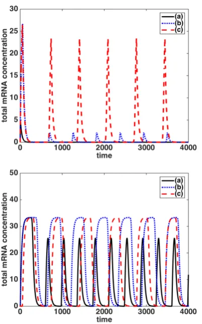
do-183

main such that:

184

∂m(−1,t)

∂x =

∂m(1,t)

∂x =0, ∂p(−1,t)

∂x =

∂p(1,t)

∂x =0,

(3)

and zero initial conditions, i.e.,

185

m(x,0)=0, p(x,0)=0. (4)

2.1. Model Parameters

186

The non-dimensional parameters, used in our

simula-187

tions are given in Table 1. These parameters are taken

188

from Sturrock et al. (2012), where a detailed discussion

189

of parameter choices is provided. They carried out a

190

full parameter analysis to determine the ranges for each

191

parameter for which oscillations were observed as well

192

as indicating how these values correspond with results

193

from the experimental literature. Our initial assumption

194

is that diffusion is a constant and the other parameters

195

are fixed. Sturrock et al. (2012) found that changes to

196

the parameters lead to changes in the nature of

oscil-197

lations, for example, changes to the period. It is

real-198

istic to expect that changes to the intracellular (and

ex-199

tracellular) environment would affect these parameters.

200

For example, changes to the transcription/translation

201

machinery due to temperature may affect the rates of

202

mRNA and protein production. Such changes would

203

then affect the period of oscillation

204

205

In non-dimensionalising the original Hes1 system (see

206

Sturrock et al. (2012) for more details) the relationships

207

between the non-dimensional parametersaand their

(4)

Parameter Description Value

D diffusion coefficient 0.00075

αm mRNA transcription rate 1.0

αp protein translation rate 2.0

µ natural degradation rate 0.03

h hill coefficient 5

ε small parameter used in 0.01

[image:4.595.69.282.108.209.2]

delta-function approx.

Table 1: Non-dimensional parameter values used

throughout our simulations. Note initially we consider

that both mRNA and protein diffuse at the same rate

such thatDm=Dp=D.

mensional counterparts [a] are given as follows:

209

D= τ[D]

L2 , αm= τ[αm]

m0 ,

αp=

τm0[αp]

p0

, µ=τ[µ],

(5)

whereτandLare a reference time and length,

respect-210

ively and m0 and p0 are reference concentrations of

211

mRNA, m and protein, p. Following Sturrock et al.

212

(2012) we takem0 = 0.0015µM and p0 = 0.001µM.

213

Taking their lead we suppose that a cell is of width

214

30µm, and as suchL = 15µm (since our domain has

215

length 2L). Equally by comparing the periods of

os-216

cillation we observe (for the Hes1 system) with

experi-217

mental data (which found the period of oscillations to be

218

2 hours, Hirata et al., 2002) we takeτ=22.5 (since

os-219

cillations occur with a period of approximately 320 time

220

units). Using these reference values the dimensional

221

parameters can be determined and are given in Table

222

2. We note that the diffusion coefficient lies within the

223

range of diffusion coefficients noted by Oeffinger and

224

Zenklusen (2012) (these varied from 0.005µm2_/_{s up to}

225

more than 1µm2_/_{s). While most of the parameters in}

226

our model are not precisely determined experimentally,

227

we note that we find the behaviour reported for ranges

228

of values for each parameter (cf. Sturrock et al. (2012)).

229

Parameter Dimensions Value

[D] µm2_s−1 ₇_.₅_×₁₀−3

[αm] Ms−1 6.67×10−11

[αp] s−1 0.0593

[µ] s−1 ₁_.₃₃_×₁₀−3

Table 2: Dimensional parameter values.

230

2.2. Varying Protein Production Site Position

231

We solve system (1), subject to the boundary conditions

232

(3) and initial conditions (4), first in Matlab using

233

the inbuilt pdepe solver and then using COMSOL,

234

with comparable results. In Figure 2 we display the

235

time-variation of the total concentrations of mRNA (top

236

panel) and protein (bottom panel). Since our interest

237

lies in whether the separation between the mRNA

238

and protein production affects whether the system

239

will oscillate, we choose to fix the mRNA gene-site

240

(at xm = 0.0) and vary the position of two protein

241

production sites (symmetric about xm). We observe

242

that if the protein production sites are either too close

243

to (solid cyan curves, xp =±0.1) or too far away from 244

(red dashed curves, xp = ±0.9) the mRNA gene-site, 245

the system will not oscillate. Instead, in both cases,

246

the system tends towards a constant level (low or high,

247

respectively) of both mRNA and protein. For the case

248

xp =±0.9, the system does initially exhibit oscillatory 249

behaviour, however oscillations are quickly damped.

250

251

For protein production sites which are adequately

252

separated from the mRNA gene-site (blue dashed,

253

black solid and green dotted curves), oscillations occur.

254

The periods we observe exhibit quite wide variation,

255

with the period increasing in proportion to the distance

256

between production sites. For example, the period

var-257

ies from 200 time units (forxp=±0.3) to 360 time units 258

(for xp =±0.7). The amplitude of mRNA oscillations 259

increases as the protein production site moves further

260

away, suggesting that an increase in separation leads

261

to higher peak levels of mRNA. However, the highest

262

peak level for the protein is observed for a mid-range

263

separation distance, e.g. xp = ±0.5. See Figure A.14 264

of Appendix A for the full space-time behaviour of

265

mRNA and protein concentrations for the Hes1 system

266

(1) withxm=0.0 andxp={±0.1,±0.5,±0.9}. 267

268

Our results indicate that separation between mRNA and

269

protein production sites can affect whether oscillations

270

occur, even for an “optimum” diffusion rate. Moreover

271

the precise distance can affect oscillation amplitudes

272

and periods. This result demonstrates that it is

im-273

portant not to neglect the spatial aspect in modelling

274

GRNs. For the purpose of discussion within this paper

275

(for our initial diffusion coefficient regime) we will

276

consider a separation distance of 0.5 length units as

277

optimum, while separations of 0.1 and 0.9 length units

278

are considered to be too short and too long, respectively.

[image:4.595.86.265.634.696.2]

(5)

[image:5.595.73.273.114.436.2]

Figure 2: Total mRNA (top panel) and protein (bot-tom panel) concentrations, for the Hes1 system, (1).

The mRNA gene-site is located at xm = 0.0 and

the protein production sites are located at xp =

{±0.1,±0.3,±0.5,±0.7,±0.9}(see legend).

2.3. Varying the Diffusion Coefficients

280

We now consider the effect of varying the diffusion

281

coefficients of mRNA and protein. Initial investigations

282

show that oscillations can be obtained for a range of

283

diffusion coefficients (as for Chaplain et al., 2015,

284

etc) but moreover that the particular combination of

285

diffusion coefficients along with position of production

286

sites dictates whether oscillations occur, and the nature

287

of oscillations. If diffusion rates, for either mRNA or

288

protein (or both) are increased/decreased, a

correspond-289

ing increase/decrease in separation between production

290

sites may also be required to generate oscillations.

291

292

In Figure 3 we indicate four separate cases, all of

293

which lead to oscillations. In the first and second cases

294

xm=0.0 andxp=±0.9, creating a separation between 295

production sites which did not lead to oscillations for

296

Figure 3: Total mRNA (top panel) and protein (bottom panel) concentrations, for the Hes1 system (1). Case (a) - solid black curve: Dm=7.5×10−3,Dp =7.5×10−4,

xm=0.0 andxp =±0.9. Case (b) - blue dotted curve:

Dm=7.5×10−4,Dp =7.5×10−3,xm=0.0 andxp =

±0.9. Case (c) - red dashed curve: Dm = 7.5×10−5,

Dp = 7.5 ×10−4, xm = 0.0 and xp = ±0.15. Case

(d) - cyan dot-dashed curve: Dm = 7.5×10−4,Dp =

7.5×10−5_,_x

m =0.0 and xp =±0.15. Note that in the

top panel (for the mRNA concentration) the solid black curve lies underneath the blue dotted curve and the red dashed curve lies underneath the cyan dot dashed curve.

our original diffusion coefficient regime (where the

297

diffusion coefficients are both equal toD, as specified in

298

Table 1). By increasing either the diffusion of mRNA,

299

in case (a), or protein, in case (b), by one order of

300

magnitude, we show that oscillations in the system are

301

now possible. In the third and fourth cases xm = 0.0 302

and xp = ±0.15, again creating a separation between 303

production sites which did not lead to oscillations for

304

the original diffusion coefficient regime. By decreasing

305

either the diffusion of mRNA, in case (c), or protein,

[image:5.595.315.517.117.431.2]

(6)

in case (d), by one order of magnitude, we show that

307

oscillations in the system are now possible. Note, even

308

when we reduce the diffusion rate of either mRNA or

309

protein by one order of magnitude, a separation of 0.1

310

remains too close to achieve oscillations. However, by

311

reducing both diffusion rates we can obtain oscillations

312

at this separation. Thus, for oscillations to occur

313

either the diffusion coefficients or gene-site separation

314

distances (or both) should be optimised.

315

316

Since mRNA molecules are smaller than protein

317

molecules, one might infer that mRNA diffuses faster

318

than protein (cf. Stokes-Einstein Law, Miller, 1924).

319

For the remainder of this paper we will discuss results

320

for two diffusion coefficient regimes. In the first both

321

mRNA and protein diffuse at a rate D. In the second

322

mRNA diffuses more quickly at a rate Dm = 0.0075

323

while diffusion of protein remains at a rate Dp = D. 324

All other parameters remain as in Table 1. For this

325

second diffusion coefficient regime we note that

oscil-326

lations are now possible at a separation of 0.9 length

327

units (and are still not found for a separation of 0.1

328

length units). See Figure A.15 of Appendix A for

329

the full space-time behaviour of mRNA and protein

330

concentrations for the Hes1 system (1) withxm = 0.0 331

and xp = {±0.1,±0.5,±0.9}, for this second diffusion 332

coefficient regime.

333

334

We repeated the investigation into the Hes1 system for

335

different geometries considering a circular, elliptical

336

and spherical domain (see Appendix B). The results

337

were qualitatively comparable, confirming that both

338

the size of the diffusion coefficients and the distance

339

between production sites (or zones) must be optimised

340

for the Hes1 system to oscillate. We note that some

341

alterations to parameters may be required as the

dimen-342

sions of the domain are increased. Armed with our

343

results for the Hes1 system we consider the role of

pro-344

duction site position in multi-gene GRNs. In particular

345

we shall study the mechanics of two types of synthetic

346

system. The first type consists of down-regulation

347

alone, where a given gene in the cycle represses the

348

next, which we will refer to as a repressilator. The

349

second type will combine both up-regulation/activation

350

and down-regulation/repression of genes. We will refer

351

to such systems as activator-repressor systems.

352

3. Synthetic GRNs: Repressilators 353

The term repressilator (first coined by Elowitz and

Lei-354

bler, 2000) has been reserved for a system of three

355

genes which couple to form a cycle of negative feedback

356

loops. We choose to use this terminology, for ease of

357

reference, for any n-gene system for which the protein

358

of any given gene inhibits the production of the mRNA

359

for the subsequent gene. Under this terminology, the

360

Hes1 system can be termed a one-gene repressilator and

361

we base our synthetic multi-gene repressilator on the

362

Hes1 system structure. As such the equations in 1D are

363

taken to be:

364

∂mi

∂t =Dm ∂2_m

i

∂x2 + αm

1+ph j

δε

xmi(x)−µmmi,

∂pi

∂t =Dp ∂2_p

i

∂x2 +αpmiδ

ε

xpi(x)−µppi,

(6)

where i = {1,2,3, . . .n} and, since the repression of

365

mRNA comes from the preceding protein in the system,

366

j={n,1,2,3, . . .(n−1)}, for ann-gene system. As

be-367

fore we use a Dirac approximation of theδ-distribution

368

function, this time located at the production sitesxmiand 369

xpi, withias above. In our simulations we consider the 370

effect of varying the position of these production sites.

371

The boundary conditions and initial conditions are, as

372

before, such that:

373

∂mi(−1,t)

∂x =

∂mi(1,t)

∂x =0, ∂pi(−1,t)

∂x =

∂pi(1,t)

∂x =0,

(7)

mi(x,0)=0 pi(x,0)=0. (8)

3.1. Two-gene Repressilator

374

We begin our analysis of multi-gene repressilators by

375

considering a two-gene (or species) system. A simple

376

schematic of a generic two-gene repressilator is shown

377

in Figure 4.

[image:6.595.356.485.547.673.2]

378

(7)

379

We solve the 1D system (6), wheren=2, with

bound-380

ary conditions (7) and initial conditions (8) using the

381

pdepe solver in Matlab (comparable results were

ob-382

tained using COMSOL). Parameters remain as for the

383

Hes1 system and are given in Table 1. By solving the

384

system for numerous production site scenarios and

vary-385

ing the diffusion coefficients, we find that the two-gene

386

repressilator system is a “weak” oscillator, in that it only

387

oscillates for a very limited set of conditions. In

Fig-388

ure 5 we provide the results for four key cases, (a)-(d),

389

under both diffusion coefficient regimes. Since we

fo-390

cus our attention solely on distinguishing between

os-391

cillating and non-oscillating cases, we choose not to

re-392

port on the behaviour of the system for the cases which

393

do not show periodic behaviour. In general, we note

394

that alternative scenarios may result in persistent high or

395

low concentrations of the mRNAs and proteins. To that

396

end we graph the concentrations of species 1 mRNA

397

only (all other concentrations behave qualitatively in the

398

same manner).

399

400

In case (a) both genes have the same production sites

401

which are optimally separated for both diffusion coeffi

-402

cient regimes (xm1 =xm2 =0.0 andxp1 =xp2=±0.5).

403

We observe oscillations, for both regimes, which match

404

closely with the oscillations for the one-gene Hes1

sys-405

tem. In this case, as we might expect, the two-gene

sys-406

tem acts just as if it were a single-gene system. Nothing

407

in the equations or numerical code distinguishes species

408

1 from species 2. In case (b) the two genes have

dif-409

ferent production sites although they remain optimally

410

separated for both diffusion coefficient regimes (xm1 =

411

±0.2,xm2 =±0.4,xp1=±0.7 andxp2 =±0.5).

Oscilla-412

tions are not observed in either regime. In case (c) both

413

genes have the same production sites with separation

414

distances only optimal for the second diffusion coeffi

-415

cient regime (xm1 = xm2 =0.0 and xp1 = xp2 =±0.9).

416

Oscillations are only seen for the second diffusion

coef-417

ficient regime. In case (d) the two genes have diff

er-418

ent production sites with separation distances remaining

419

optimal for only the second diffusion coefficient regime

420

(xm1 =0.0, xm2 = ±0.1, xp1 = ±0.9 and xp2 = ±1.0).

421

In this case neither diffusion coefficient regime leads to

422

oscillations. Our investigations indicate that if the

pro-423

duction sites for the two genes are different then

oscil-424

lations will not occur, regardless of whether gene-site

425

position and diffusion coefficients are optimum or not.

426

Oscillations may only be obtained if the two genes share

427

the same production sites, when the system effectively

428

behaves like a one-gene repressilator, the Hes1 system.

429

However, in such a case, the separation between

[image:7.595.315.517.115.436.2]

pro-430

Figure 5: Total mRNA concentrations for species 1 for the two-gene repressilator under both diffusion coeffi -cient regimes. Top panel: first regime,Dm =Dp = D.

Bottom panel: second regime,Dm =0.0075 andDp =

D. Case (a) - solid black curve: the production sites are

xm1 = xm2 = 0.0 and xp1 = xp2 = ±0.5. Case (b)

-blue dotted curve: the production sites arexm1 =±0.2, xm2 =±0.4, xp1 =±0.7 andxp2 =±0.9. Case (c) - red

dashed curve: the production sites arexm1 =xm2 =0.0, xp1=xp2=±0.9. Case (d) - cyan dot-dashed curve: the

production sites arexm1 =0.0,xm2 =±0.1,xp1 =±0.9

andxp2=±1.0.

duction sites must then be optimised in relation to the

431

diffusion coefficients in order to obtain oscillations. In

432

support of these results we note that we have obtained