Encoding of relative location of intensity changes in human spatial vision

(1)

ENCODING OF RELATIVE LOCATION OF INTENSITY

CHANGES IN HUMAN SPATIAL VISION

Ian R. Paterson

A Thesis Submitted for the Degree of PhD

at the

University of St Andrews

1992

Full metadata for this item is available in

St Andrews Research Repository

at:

http://research-repository.st-andrews.ac.uk/

Please use this identifier to cite or link to this item:

http://hdl.handle.net/10023/14594

(2)

Encoding of relative location of intensity changes

in human spatial vision

Ian R. Paterson

August 1990

University of St. Andrews

Scotland

(3)

ProQuest Number: 10167235

The quality of this reproduction is dependent upon the quality of the copy submitted. In the unlikely event that the author did not send a com plete manuscript and there are missing pages, these will be noted. Also, if material had to be removed,

a note will indicate the deletion.

uest

ProQuest 10167235

This work is protected against unauthorized copying under Title 17, United States C ode Microform Edition © ProQuest LLO.

ProQuest LLO.

789 East Eisenhower Parkway P.Q. Box 1346

(4)

(5)

In submitting this thesis to the University of St. Andrews I understand that I am giving permission for it to be made available for use in accordance with the regulations of the University Library for the time being in force, subject to any copyright vested in the work not being affected thereby. I also understand that the title and abstract will be published, and that a copy of the work may be made and supplied to any bona fide

(10)

Declaration for the degree of Ph.D.

I, Ian Robert Paterson, hereby certify that this thesis has been composed by myself, that it is a record of my own work, and that it has not been accepted in partial or complete fulfilment of any other degree or professional qualification.

Signed: Date: S i

I was admitted to the Faculty of Science of the University of St. Andrews under Ordinance General No. 12 in October, 1986, and as a candidate for the degree of Ph.D. in 1990.

Signed: Date: /|U |

I hereby certify that the candidate has fulfilled the conditions of the Resolution and Regulations appropriate to the degree of Ph.D.

Signature of Supervisor: Date:

(11)

Chapter 0: Introduction

Chanter 0

Introduction

(12)

-Chapter 0; Introduction

0.1: Preamble

One view of how we should study vision holds that only analysing what information is available to the visual system to perform a task is liable to deliver meaningful results (Watt, 1990; Marr, 1982). However, there is a venerable tradition of trying to understand something about our psychological experience of the world in terms of theories of one sort or another, and it may be that our understanding of vision can be increased by studying some of the subjective aspects of vision, at least if done carefully enough, with due regard for the perversity of human psychology.

The study is a psychophysical investigation of the perception of relative spatial location. A great deal is known about how the human visual system assesses the relative location of image features, but there are some aspects of relative localisation which have not yet been fully understood, and to date no comprehensive explanations exist of the geometric illusions. This study was an attempt explain some very simple geometric distortions using soundly based principles of low-level vision. The experiments reported here involved measuring location biases and precision on relative localisation tasks. From spatial interference experiments, it was found that changes in perceived location induced by the presence of flanking features can be explained by MIRAGE (Watt & Morgan, 1985); interference with both vernier acuity and direction of displacement discrimination, the difference between the data from these tasks, the differing pattern of spatial interactions between bars and edges, and the effects of blur on these tasks are explained by MIRAGE in elegant fashion.

(13)

s Chapter 0: Introduction

demands it. A dissociation is found between the phenomenology of perceived separation of luminance features and the information necessary to judge their separation. Combination of information across spatial scales was implied by the

pattern of biases measured for stimuli without spatial perturbation, but could not be 1 reconciled with the precision of separation judgments for stimuli with spatial

perturbations. When the stimuli does not vary randomly in its spatial configuration, the system appears to combine information across several scales, but when there is externally applied noise on the coarser scales that the system can identify as noise, then it can restrict itself to using information present only on a fine scale. This closely parallels an observation by Burbeck & Yap (1990), indicating that the visual system

can choose to accept information only from spatial scales which deliver a reliable | signal which is task-related, indicating a role for selective attention even at the earliest

stages of edge localisation.

0.2: Early vision

The general framework of this investigation is based upon ideas developed by David Marr (1976, Marr & Hildreth, 1980; Marr, 1982) and Watt and Morgan (1984,1985) who applied his approach to the study of early vision. Marr (1982) stressed that a complex system may only be understood if a number of levels of analysis are simultaneously brought to bear on the system. He argued that for a problem as complex as biological vision to be understood, it necessarily should be understood at the levels of computational theory, algorithms and hardware. His main point was that the computational theory should guide research at the other levels. The computational theory states what is being computed, and why it is being computed. It should specify what sort of representations are necessary (ie. what information is made explicit at a given stage in processing) and how the information in a representation is manipulated by the processes which act upon it. The algorithmic level gives details of how to implement the theory, which is likely to be hardware- dependent; the computational theory ought to be hardware-independent. Marr believed that given the complexity of the neural architecture, an understanding of what the brain did would not arise by direct examination of what it looked like and what it

appeared to be doing, but rather by a rigorous study of the information necessary for a |

task and how the task might be carried out. Central to Marr's ideas is the belief that early processes are largely data-driven; the visual system is thought to be concerned with squeezing as much information necessary to make a correct interpretation out of

(14)

Chapter 0: Introduction

the image before any higher-level processes are involved. A representation is simply a means of encoding information- a description of some sort, which may make explicit properties of the visual scene which are not obvious upon examination of the intensity distribution of the image (eg. the location of texture boundaries, for instance).

Marr regarded early vision as a set of computational processes which detect and 4 represent intensity changes in the image, extract information about local geometric i

structures in the image, and detect and analyse the effects of illumination (eg. determining whether a surface is opaque or transparent). He viewed the ultimate aim of early vision as construction of a visible surfaces representation (the so-called '2.5 D sketch', which is a viewer centred description of the visual image), in which surface attributes such as orientation and relative distance from the viewer might be made explicit, based upon combining information from stereo, motion, shading,

shadows, texture, intensity and chromatic changes. The most primitive representation A in Marr's scheme is the primal sketch (which Marr subdivided into 'raw' and 'full'

primal sketches), which is retinotopically organised. The primal sketch is composed of a set of spatial primitives. In Marr's scheme, spatial primitives, are cousins to Lotze's (1884) retinal mean local signs. Spatial primitives encode attributes of image features as edge/ boundary segments, bars, feature terminations and 'blobs' (doubly terminated bars). These primitives in turn are acted upon by early grouping processes (which embody prior knowledge that the visual system has about the geometry of the visual world). Marr and Hildreth (1980) devised a scheme for detecting and representing intensity changes in the retinal imge, based on a number of bandpass spatial frequency filters which are used to analyse the retinal image in parallel. The outputs of the filters are combined and features in the combined output extracted to give a 'raw primal sketch* of the image. Watt and Morgan (1984, 1985) applied a related model to data from extensive psychophysical experiments to explain performance on relative localisation tasks. These models are described in the next chapter. Most models in computational vision which have as initial stages in their operation filtering by spatial frequency bandpass filters; extensive work on multiple spatial frequency channels and spatial contrast detection, started by Campbell and Robson (1968), indicates the existence of multiple spatial frequency bandpass filters at each retinal locus in the human visual system. The evidence for this notion is described in the next chapter.

10

(15)

Chapter 1: Studying early vision

Chapter One

Studying early vision

(16)

Chapter 1; Studying early vision

1.1: Overview

The purpose of this chapter is to discuss psychophysical and theoretical work relating to how the human visual system detects and represents elementary image features, and computes spatial relations amongst such features. Psychophysical data and theory relating to detection and discrimination of contrast-modulated patterns is discussed in the sections 1.2 through 1.6. The literature is vast, even when attention is confined to static, achromatic luminance modulated patterns, and the account here is inevitably highly selective. Section 1.2 presents empirical evidence for the existence of multiple spatial frequency bandpass filters in early vision, derived from studies of the visual system’s sensitivity to spatial modulations of luminance; the existence of such bandpass filters is central to most theories of low-level vision.

There are many different pattern acuities which have been investigated- a pattern acuity is simply the limit on precision in judgments about elements of the geometr y of one or more pattern(s). Measures of precision can be highly informative, since precision (the reciprocal of the subject’s error variance) is a direct measure of the amount of information the system has available in performing the task. Ideally, we wish some mathematical model, which should explain why the human observer shows the pattern of information loss which they do (Watt & Morgan, 1983b). A major part of the task of psychophysics is to discover what cues subserve psychophysical judgments, a cue simply being an information source. Section 1.3 describes results from studies of vernier acuity and orientation discrimination. The

following section, 1.4, is an account of data from spatial interval and spatial f* frequency discrimination experiments; these sorts of discriminations are relative

localisation tasks which display fundamental differences to vernier acuity. Unlike

vernier acuity, spatial interval discrimination is remarkably robust to changes in the 'I spatial configuration of the target. Psychophysical evidence for the existence of

spatial primitives in human vision is discussed in section 1.5. Section 1.6 samples some theoretical accounts of early visual processing; section 1.7 is a very brief account of some of the neurophysiological research which is relevant to psychophysical studies of early vision. Whilst several workers have attempted to make close links between physiological and psychophysical results, it seems ambitious at this stage in our knowledge to do so. To date, there are no neurobiological linking hypotheses which allow reconciliation of psychophysical and neurophysiological results. On the other hand, physiology and anatomy can identify constraints on what sorts of representations and processing occur in

(17)

1.2.1: The multiple spatial frequency channel model

There is ample evidence that neural mechanisms exist in human vision, which correspond to bandpass spatial frequency selective mechanisms (Campbell & Robson, 1968; Blakemore & Campbell, 1969) and which are also spatially localised (Wilson & Bergen, 1979). Several different spatial scales are believed to co-exist at each retinal location ( Graham, Robson &Nachmias, 1978; Wilson & Bergen, 1979).

The proposal that the visual system might be transmitting independent spatial frequency signatures of the retinal image was made by Campbell and Robson (1968). They determined how well subjects could distinguish a square wave modulation of contrast from a sine wave grating; they concluded that "a square wave grating is perceived to be different from a sine-wave grating when the third harmonic of the square wave independently reaches its own threshold." They explicitly compared the visual system to a linear system and proposed that early vision literally performs a Fourier analysis of the retinal image. Blakemore and Campbell (1969) determined contrast thresholds for gratings following adaptation to a high contrast grating, and found that thresholds were elevated only for frequencies near to the adapting frequency, which they interpreted as a selective

14

■i

biological visual sytems. Additionally, neurophysiological results have been used to generate models of relative localisation of image features, and some of these models are briefly examined in this section.

1.2: Spatial contrast detection and multiple channels theory

This section discusses briefly some of the psychophysical evidence in favour i of multiple, spatially coincident and relatively independent spatial filters in

human vision. Most empirical evidence on the nature of 'channels' has come from studies of spatial contrast detection (using adaptation, subthreshold summation,

masking and other related paradigms) where the contrast of the lowest contrast * pattern that can just be seen is determined as a function of the stimulus parameters.

The most difficult problem with such studies is that it is hard to generalise the results | to suprathreshold contrast levels. There has has been an extensive and systematic

(18)

impairment of a subset of the visual system's spatial frequency channels. Graham

and Nachmias (1971) demonstrated that the detectability of a compound grating :j composed of more than one sinusoidal component did not depend on the relative

phase of the components. Sachs, Nachmias and Robson (1971) interpreted their data as evidence that unless gratings are very similar in frequency, they are detected by independent spatial frequency selective filters.

1.2.2: A space-variant single-filter model

All of the data presented above could be explained by a model in which the frequency components of spatially extended patterns like gratings are independently detected at different visual field locations. From psychophysical (Green, 1970) and physiological (eg. Hubei & Wiesel; 1962, 1974a, 1974b) evidence, the visual field is known to be markedly inhomogeneous, with a general increase in the spatial scale of receptive fields at more peripheral locations. It is possible that the relatively independent detection of widely separated frequency components requires the components to be detected at different retinal locations. The sensitivity of central vision to fine spatial detail (ie. information conveyed by high spatial frequencies) has long been known, and it is possible that low spatial frequency components could be detected at more peripheral visual field locations. A model incorporating the inhomogeneity of the visual field was devised by Limb and Rubinstein (1977). This model incorporated a single linear filter at each retinal location, but the scale of the filter increased with eccentricity. Since the filter was linear, its response could be described by a convolution with the input pattern. Their filter parameters were derived from measurements of the sensitivity of the visual system to two line patterns separated by different distances, which they used to determine a one dimensional line-spread function (spatial weighting or sensitivity function) at six different eccentricities (0-8.3 deg arc). The filter profile had a large number of free parameters to ensure a good fit to the sensitivity data. They then predicted thresholds for other classes of patterns (eg. bright/ dark bars, gratings) using this space-variant single filter model; the model was quite successful in explaining all the data from

their experiment. Energy summation across spatial frequency is predicted by a single % lienar filter model; presenting stimuli with substantial energy at two widely separated

(19)

%

1.2.3: Evidence for multiple spatial filters at one locus

Subsequent studies showed that there is more than one scale of spatial filter at each 4;

retinal location. Graham, Robson and Nachmias (1978) measured summation of 4

sinewave gratings of different frequencies, for patches of grating windowed with a

Gaussian to localise the stimulus in a particular retinal region (presented either | foveally or 7.5 deg peripherally), in order to minimise the confounding effects of

retinal inhomogeneity on detection. The grating patches were composed of gratings of 2 and 6 c/deg, in either 0 or 180 deg relative phase (peaks-add and peaks- subtract, respectively). The detectability of the f-3f compound is less than would be expected if one linear filter were present at each retinal locus (as in the model of Limb and Rubinstein); detection of the different components was slightly better than predicted by a wholly-independent filter model, which they attributed to probability summation across spatial frequency detectors (eg. a filter with a peak frequency of 4 c/deg has some probability of responding to a grating of 6 c/deg or 2 c/deg).

If patterns are presented at contrast threshold, then discrimination may require that the patterns are detected by different filters; ie. that somehow the filters are labelled', although this is a strong assumption. Watson and Robson (1981) used a detection/ identification paradigm to examine spatial frequency discrimination for Gabor patches (sinewave windowed with a Gaussian) presented at contrasts near to detection threshold. In this paradigm, the subject is required to indicate which of two temporal intervals contained the grating patch, and whether it was of the higher or lower of the two spatial frequencies being presented within any one session. To give 'perfect' discrimination at contrast threshold (being when the grating is correctly identified every time it is detected), a difference in spatial frequency of about an octave between the patches was necessary. Watson and Robson concluded that about seven classes of independent local spatial frequency detectors were necessary to explain performance on these tasks, if errorless discrimination depended on signals from labelled filters with different peak spatial frequencies.

Wilson and Bergen (1979) developed a highly influential model of threshold spatial vision, based on the operation of four independent spatial frequency filters at each retinal location; this is described in section 1.6. The peak frequencies of the filters in Wilson and Bergen's model ranged from 1-8 c/deg. An experiment by Watson (1982) suggested the need for a wider frequency range of filters than those in Wilson and Bergen's model. Watson presented compound grating patches spatially

(20)

windowed with a Gaussian; the higher of the two component frequencies in the patch was varied, and the detectability of the compound patch measured. The lower frequency was either 1 or 16 c/deg. Watson measured less summation than would be predicted by the filters from Wilson and Bergen's model, indicating relatively independent detection of Ic/deg and 2.8 c/deg patches was occurring (as well as for

16 c/deg and 32 c/deg patches).

1.2.4 Fourier analvsis and earlv vision

The view of early vision as equivalent to a Fourier analysis of the retinal image was the dominant paradigm in spatial vision for many years. From a computational perspective, this is not really a theory of vision at all. Fourier analysis allows an arbitrary waveform, as long as it is limited by physical possibility, to be re-expressed as the sum of periodic components. Fourier methods transform a waveform expressed as a function of space and/or time into an equivalent representation in the frequency domain. Fourier analysis can describe the response of all systems that are linear and stationary (time-invariant). The Fourier transform of a waveform can be expressed as a sum of sinusoids with different frequencies; each frequency has an associated amplitude (or energy) and phase.

Descriptions in the frequency domain and space domain are formally equivalent; no information is sacrificed by a Fourier transform, but the only useful property of a simple Fourier transform for an image analysis sytem is that the transform gives a shift-invariant representation if (and only if) the phase spectrum is ignored. Since the phase spectmm carries information about local image geometry, this neglect leads to problems. In terms of Marr's approach, there appears to be little made usefully explicit in transforming the image into a frequency representation. It might be argued that with high spatial frequencies generally carrying texture, low spatial frequencies 'shape' there is some useful partitioning of image information; but we do not need an exclusively frequency domain representation to do this- we can do this equally well with multiple spatial scales of representation. One major problem with the work on spatial contrast detection was that it was driven by the idea that early vision performed a spectral analysis of the input, and that the system was essentially linear. The models

(21)

threshold contrast patterns to make accurate predictions about visual responses made at suprathreshold contrast levels (Olzak & Thomas, 1987).

1.3: Relative localisation

There are many sorts of acuities, the most frequently encountered being resolution acuity - ability to see fine spatial detail; for instance, to tell that two dots are separate, or see a high spatial frequency grating pattern. The lowest values obtained for resolution acuity are in the order of 30 sec arc, or close to the diameter of a foveal cone. There are other sorts of pattern acuities which yield finer thresholds than this; vernier thresholds, for instance, can be as fine as 3 sec arc (Westheimer & McKee, 1977a); since this is about one-tenth of the diameter of the smallest photoreceptors, the processing underlying vernier acuity is a form of neural interpolation (Barlow,

1981; Morgan & Watt, 1982).

1.3.1: Vernier acuitv and mean retinal sign

One familiar result in vernier acuity is improvement in sensitivity to vernier offset as the length of the lines in the target is increased. For abutting targets, there is a limited dependency of vernier acuity on line (or edge) length (Anderson & Weymouth, 1923; Andrews, Butcher & Buckley, 1973; Westheimer & McKee, 1977a). The spatial scale of the target determines the retinal distance over which increasing the feature length can improve vernier acuity. Watt and Morgan (1983b) demonstrated that the region over which target length can improve performance is proportional to the blur of the target features. For instance, with edges having a space constant of 10 min arc, they found that an edge length of 1 deg is necessary for asymptotic performance. For fine line targets, vernier threshold is almost independent of line-length beyond an overall target length of about 10 min arc (Westheimer & McKee, 1977a).

The dependence of vernier acuity on line-length was used by Hering (1899) to explain the precision of vernier acuity, which he saw as resulting from averaging across the length of the lines in a vernier target to derive a retinal mean local sign for each line. This notion of a local sign is based on information in the retinal intensity distribution itself, but more recent forms of this idea are based on information in blurred and differentiated versions of the retinal image, although the fundamental concept is the same- representing an image feature by a 'token' or symbol of some sort, which itself possesses only a limited amount of information. Evidence for

(22)

1.3.2: Two mechanisms in vernier acuitv

Ludvigh (1953) showed that two dot vernier acuity can be as precise as two line vernier acuity, which refutes the notion of a mean local retinal sign as the only explanation of the precision of vernier alignment. It is also possible to use a relative orientation cue in performing a vernier task. Relative to an aligned target, a vernier target with an offset appears as rotated slightly (eg. rotated clockwise if the lower bar is offset to the left of the upper bar). Vernier acuity may reflect the operation of at least two localisation mechanisms, one concerned with extracting an overall orientation for an image feature, and the other with extracting information about the relative location of the components in the target, in the dimension perpendicular to the main axis of the target. Evidence for the existence of two distinct mechanisms involved in vernier acuity was provided by Watt, Morgan and Ward (1983a). In a conventional vernier task (eg. judging whether one line above the other is offset to the left or right), the subject may use both the relative orientation of the target (eg. relative to vertical) and the relative location of the components of the target in judging the direction of vernier offset. If the orientation of the target is varied randomly from trial to trial, then the relative orientation cue becomes unreliable, (| since a change in perceived orientation is not related to the direction of offset.

Performance on the vernier task should then be determined by the operation of the mechanisms which compare local signs for the target elements. Ideally, we would like to show a relation between physical cue amplitude and precision of localisation- ie. to discover what physical cue controls localisation precision; if we degrade a given cue and localisation performance deteriorates in a systematic fashion, we can assert that information carried by this cue is necessary for localisation (since precision of localisation is inversely related to the amount of information used by the system). For a conventional vernier judgment, comparison of local signs will have to occur along the direction perpendicular to the main axis of the target; ie. in the "orthoaxial" direction (Watt & Andrews, 1982). We can degrade the orthoaxial contrast information available to the system by blurring the target. This was performed by Watt, Morgan and Ward (1983a); they blurred the corners of an spatial primitives comes from studies showing that primitive features of a given sort

result in a comparable information loss to that shown by the human visual system in | making a judgment- that is, by demonstrating that precision in a given task declines

(23)

1

abutting vernier target, and determined vernier thresholds for various degrees of comer blur. When sharp corner detail is present, randomising the reference orientation (with the overall target length constant at 30 min arc) has no effect on vernier thresholds. Blurring the corner detail leads to a difference between the random and fixed reference orientation conditions, for greater degrees of corner

blur. The decline in performance seen in the random slope condition (when 4 no relative orientation cue is present) is consistent with the degradation in the

amount of orthoaxial contrast information present in the target. It is therefore

reasonable to conclude that this information is used by at least one of the 2* mechanisms involved in vernier acuity.

1.3.3: Orientation discrimination

Orientation discrimination is another sort of pattern acuity which is capable of yielding thresholds in the 'hyperacuity’ range; a change in orientation for a pattern of as small as 0.5 degrees rotation can be detected by the visual system, which for short lines yields thresholds of less than a cone-diameter, ie. in the hyperacuity range. Despite a superficial similarity to vernier judgments, there are some quite striking differences between orientation discrimination and vernier acuity.

Like vernier acuity, orientation discrimination is dependent on line length (Andrews, 1967) with improvements reported at line lengths of at least one degree of arc for an abrupt 1 msec ("transient") presentation, and up to 30 min arc for "continuous" presentation (unlimited inspection time). Spatial interference with orientation discrimination has a similar pattern to interference with vernier acuity (Westheimer, Shimamura & McKee, 1976), with optimal interference occuring when two symmetrically disposed flanking lines are situated some 3-6 min arc distant from the target line.

Orientation discrimination improves over part of the contrast range, but performance saturates at relatively low contrasts of about 5-10% (Regan & Beverley, 1985; Skottun, Bradley, Sclar, Ohzawa & Freeman, 1987). This makes it somewhat different to vernier acuity, which is dependent on contrast for the whole of the contrast range (Watt & Morgan, 1984). Another difference is that orientation discrimination thresholds are largely independent of spatial frequency (Heeley & Timney, 1987), unlike vernier acuity, which is related to the spatial scale of the targets to be localised (Watt & Morgan, 1984; Bradley & Skottun, 1987). There is

(24)

some evidence that orientation discrimination is unaffected by the presence of a large spatial frequency difference between the stimuli to be compared (Bradley & Skottun, 1984), although this may be artefactual (Heeley, pers. comm.). Both orientation discrimination and vernier acuity display meridional anisotropies (McKee & Westheimer, 1978; Heeley & Timney, 1987; Orban, Vandenbussche & Vogels,

1984; Corwin, Moskowitz-Cook & Green, 1977), which may reflect the use of a relative orientation cue in the vernier task becoming less effective at oblique orientations.

1.4: Spatial frequency and spatial interval discrimination

One school of thought (Olzak & Thomas, 1987) regards spatial frequency discrimination as a degenerate case of size discrimination (in which the stimulus is highly redundant), since the width of bars in a grating are inversely related to the spatial frequency. This section treats spatial frequency discrimination as a spatial interval discrimination between bars of the same contrast polarity in the grating target. Spatial period discrimination reaches an asymptote at 1.5 cycles of a sinewave grating (Hirsch & Hylton, 1982), suggesting that optimal performance can

be based on just one spatial interval (eg. between two bright bars in the grating %

(25)

1.4.1: Precision and perturbation

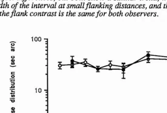
The precision of both spatial frequency and interval discrimination is surprisingly resistant to changes in the luminance profile of the retinal image that are known to be important in detection tasks, which immediately suggests difficulties in attempting to explain precision of such discriminations in terms of the properties of low-level detection mechanisms (eg. WiUon & Gelb, 1984). Fractional thresholds for spatial frequency discrimination are relatively constant over a wide range of spatial frequencies (Campbell, Nachmias & Jukes, 1970), in contrast with the dependence of sinusoidal grating visibility on spatial frequency (Blakemore & Campbell, 1969). Fractional difference thresholds are similar across a wide range of spatial frequencies at very low contrasts if the stimuli are equated for visibility (Thomas, Gille & Barker, 1982; Watson & Robson, 1981). Campbell et al (1970) found no significant difference in discrimination thresholds for square versus sinewave gratings, and no superiority for binocular over monocular presentation. Spatial frequency discrimination thresholds are known to be independent of contrast over most of the contrast range. Caelli, Brettel, Rentschler and Hilz (1983) measured frequency discrimination thresholds at contrasts ranging from 5 to 25 % contrast, at different reference orientations and frequencies, and found no effect of contrast, replicated by Skottun, Bradley, Sclar, Ohzawa and Freeman (1987) for a wider contrast range. Morgan and Regan (1987) demonstrated that precision of spatial interval discrimination is unaffected by a contrast randomisation procedure (for separations greater than 2.5 min arc). Similarly, edge blur width discrimination , wherein subjects are required to estimate the spatial extent of a blurred edge, is unaffected by contrast randomisation (Hess, Pointer & Watt, 1989).

Spatial interval discrimination is relatively robust to changes in the spatial configuration of the target. Two point separation discrimination is as good as that for line separation (Westheimer & McKee, 1977a). Morgan and Ward (1985) determined spatial interval thresholds for intervals with flanking features placed a randomly varying distance either side of the interval delimited by two lines; this manipulation did not affect the precision of interval judgments.

Spatial interval discrimination is also apparently insensitive to the spatial frequency composition of the individual features delimiting the interval. Burbeck (1988) devised spatial interval targets which were delimited by either lowpass Gaussian bars, or high-frequency bandpass modulated bars, or one of

(26)

each. She reported that interval discrimination was as accurate with the mixed frequency pairs as with those matched in frequency. Likewise, Toet and Koenderink (1988) found that the frequency content of a Gabor patch had no effect upon the thresholds for spatial bisection and displacement tasks with three "blob" targets, whose intensity profile was a two-dimensional Gaussian function, presented at threshold contrast. Bradley and Skottun (1984) and Burbeck and Regan (1983) both reported an apparent insensitivity of spatial frequency discrimination to the presence of a 90 deg. orientation difference between the gratings to be discriminated. Additionally, spatial period discrimination is largely unaffected by duration of the inter-stimulus interval; Regan (1985) showed no decline in precision of period estimation for inter-stimulus intervals of up to twenty seconds. Judgments are robust to variations in the relative distances between the comparison stimuli (Campbell, Nachmias & Jukes, 1970), and contrast randomisation (Heeley, in press). Spatial interval discrimination can be as precise in a single interval judgment, where the subjects must compare the width of the target stimulus with some internal standard, acquired through feedback (Westheimer & McKee, 1977a).

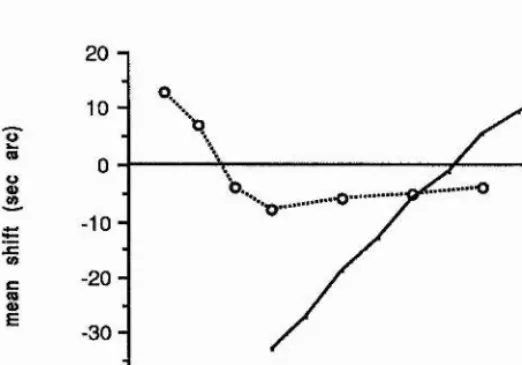
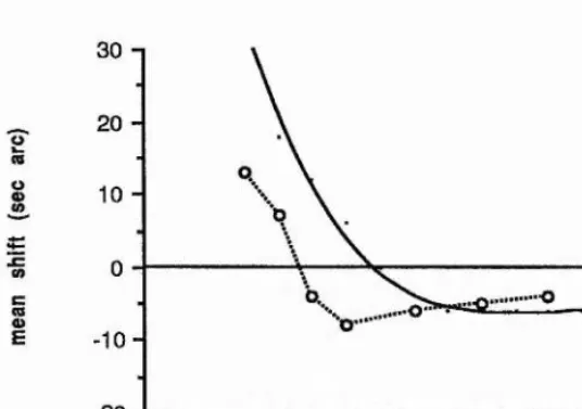
Beyond small separations, accuracy of interval discrimination is not affected by the polarity of contrast of the features delimiting the interval. Discrimination of small and large separations may be performed by somewhat different processes; Levi and Westheimer (1987) showed that interval discrimination for lines of different polarities is poorer than for lines of the same polarity when the separation is small (ie. less than about 4 min arc), and this is supported indirectly by the result of Morgan and Regan that contrast randomisation of the bars in the interval target did affect interval discrimination at the smallest separation they used (2.5 min arc).

1.5: Psychophysical evidence for spatial primitives

(27)

judgment with fine, bright lines. They presented narrow bars (less than 3 min arc wide); one of the two bars had a luminance asymmetry, and subjects were simply asked to perform a vernier alignment of the two bars. Subjects could accurately discriminate the relative location of the centroids of the two bars (with a precision equivalent to ’normal' vernier acuity for symmetric bars) without being aware that the bars were asymmetric in luminance. Whether the subjects were actually estimating the location of the centroid of the retinal intensity distribution was not clear- it is possible that some other feature (which happened to fall close to the location of the centroid of the intensity distribution for these stimuli) was being used, but they did not distinguish between any alternative candidates.

1.5.1: Zero-crossings

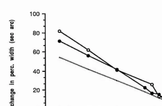
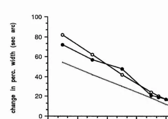
The first empirical demonstration of the perceptual significance of zero-crossings in the second spatial derivative of a smoothed version of the image was provided by Watt and Morgan (1983a). They measured the perceived width of narrow, bright bars with a luminance asymmetry, relative to a symmetric bar. Luminance asymmetries were created by having two very narrow bars with differing luminances spaced below the resolution limit. Subjects could discriminate the 'paired' bar from a single bar, when the change in the separation of the peaks of the two bars was much less than the theoretical resolution limit for these two stimuli (about 1 min arc); subjects were discriminating the width of the paired bar and the single bar, and these width thresholds increased as the degree of luminance asymmetry in the 'paired' bar increased.

They examined whether zero-crossings in the second derivative of a smoothed retinal image could explain the thresholds for changes in perceived width of these asymmetric bars. They simulated the neural response with a DOG filter (centre- surround ratio 1:1.75, excitatory centre space constant 22 sec arc). Zero-crossings accounted for the width thresholds obtained with these asymmetric stimuli. Other candidates for edge primitives they discounted were threshold edges (places in the image where the luminance exceeds some threshold value) and luminance maxima; these intensity features made predictions which were inconsistent with the results of vernier acuity for targets composed of one symmetric and one asymmetric bar, relative location in the vernier task depending on either the mean of the intensity distribution, or the zero-crossings in the 2nd derivative of the smoothed image. They could not choose between the mean/ zero-crossings models on the basis of the

(28)

i vernier acuity data, since the largest luminance asymmetries they could create did not J lead to predictions discriminable within experimental error, but only the zero-

crossings model could explain the bar-width discrimination data.

1.5.2: Centroids and extrema

In a further set of experiments Watt and Morgan (1983b) examined the suggestion of Marr and Hildreth (1980) that edge blur and contrast could be computed from the

scale of filter responding to an edge, and the gradient of the filter response at the | zero-crossing (in the direction perpendicular to the 'edge' alignment). Marr and

Hildreth's edge primitives were zero-crossing segments and associated gradients of I the normals to these segments, computed by filtering the image with several scales

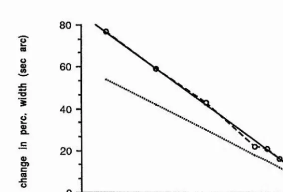
of second-order filters. Watt and Morgan determined thresholds for detecting a change in the spatial extent of blurred step edges, which had either Gaussian, rectangular or cosinusoidal blurring functions. They noted that sensitivity to an increment of blur added to a sharp edge is less than an increment added to a slightly more blurred edge, which was one of the critical pieces of evidence for their theory of spatial primitives MIRAGE (Watt and Morgan, 1984, 1985); this indicates the addition of some degree of internal 'blur' to an edge, which is consistent with the responses of larger scale filters being combined in some way with the smaller scale filters to increase the effective neural blur. For blur extents of less than about 3 min arc space constant, threshold increases with decreasing blur extent.

(29)

Watt and Morgan note is a remarkable coincidence. For separations of the extrema in the second derivative of the retinal stimulus of greater than 5 min arc, a power law with an exponent of 1.5 fits the data for the three different blur types and the functions have the same height above the x-axis. The simplest way of describing their data is the following function,

A S

S y =--- for values of S > 5 min arc

where = the blur extent difference threshold, A = a constant

C - contrast S = pedestal blur

They dismissed Marr and Hildreth’s suggestion that edge blur could be computed from the scale of filter responding, since this scheme would predict that edge blur thresholds for rectangular blur of medium and greater blurs would be much poorer than they were (since the smaller scale filters would not give zero-crossings in response to moderately blurred rectangular edges). The gradient at the zero-crossing in the second derivative of the retinal stimulus cannot be a cue to blur extent; since this is proportional to blur extent and inversely proportional to contrast, then the power law exponents for the effects of pedestal blur and contrast should be equal in magnitude but opposite in sign (whereas they are different in reality by a factor of three).

They also measured localisation thresholds for blurred edges, using a vernier task. Vernier thresholds were measured for edges with Gaussian, rectangular and cosinusoidal blur, as functions of both contrast and edge blur. Vernier thresholds showed an inverse square root dependency on contrast, and a square root relationship with edge blur. To explain this data, a very simple statistical model was devised; they equate the task of finding the extrema of a zero-bounded filter response distribtion, which is a portion of the blurred second spatial derivative of the retinal image, with finding its first moment (centroid). By analogy with the process of estimating the mean of a distribution, where the precision of the estimate of the mean is given by the standard error of the mean (the standard deviation divided by the square root of the number of samples), the precision with which this centroid can be

(30)

located will depend on both the dispersion of this distribution and on the area of this response distribution, the dispersion of the distribution being equivalent to the standard deviation, and the area under the distribution the number of samples (from this analogy). The area of the distribution will depend on both contrast and edge blur, but they assume the width depends only on edge blur.

Their working is shown below.

From their analogy,

where S is the theoretical localisation threshold (the s.d. of the error response distribution) k = a constant

W = the width of the zero-bounded response distribution

A = the area of the zero-bounded response distribution

Since the area depends on both contrast and width, A = k’.W.C

we can substitute in the above equation for A and simplify, giving

Vw

S = c. where c is a constant

which was the observed relationship between the stimulus parameters and the psychophysical threshold; expressing localisation thresholds as a function of stationary point width (at 80% contrast) gave a threshold which showed a square root dependency on the stationary point width. The inverse square root relationship of threshold to contrast has been discussed above.

1.5.3: Interpreting primitives

(31)

deciding which positive centroid goes with which negative centroid, but this will not be generally true for natural images. They propose that a region of zero-filter response between pairs of centroids of opposite sense is necessary to allow segregation of the features corresponding to distinct edges or bars; in other words, to solve the correspondence problem for the features which together represent the edge. This is a neat way out of what could be a tricky computational problem, and is supported indirectly by several brightness illusions, which can be explained by supposing that the system fails to register the "true" nature of the visual image if there is either an absence of a zero-region between positive and negative centroids which do not belong to the same edge, or if there is a fortuitous region of zero- response between features which should belong together. In the Chevreuil illusion, consisting of two closely spaced step edges, three edges are seen instead of two, but this is only true for small spacings of the two step edges; consistent with the system failing to resolve a region of zero-response between two centroids of opposite sense which do not belong to the same edge. Mach bands can be seen for ramp edges, but not at very small sizes of ramp, consistent with the system adding in extra edges of opposite polarity in situations where features which should be kept separate are incorrectly combined into edge-primitives.

1.5.4: Perceived size and spatial extent

Many studies have looked at changes in perceived spatial frequency; for instance, following adaptation (Blakemore, Nachmias & Sutton, 1971; Heeley, 1979) or shifts in perceived frequency due to changes in contrast (Georgeson, 1980). The rationale for these experiments has typically been to demonstrate that perceived spatial frequency or size can be explained by the relative activity of spatial frequency tuned channels. Gelb and Wilson (1983a,b) tried to explain perceived size in terms of such frequency channel models, but found them unable to account for many observations relating to the perception of the size of spatially localised patterns.

Gelb and Wilson (1983a,b) studied changes in the perceived size of spatially localised Difference-of-Gaussian (DOG) patterns produced by varying contrast, temporal modulation or by the presence of a masking sinewave grating. The effect of reducing the contrast of a DOG pattern is to reduce its perceived size relative to a high contrast standard, also observed by Georgeson (1980) for Gaussian bars. These results held under both sustained and transient temporal modulations. To attempt to explain their results, they employed a model for perceived size based on

(32)

earlier formulations by Klein, Stromeyer and Ganz (1974) and Georgeson (1980), using filter space constants and sensitivity parameters from Wilson and Bergen (1979).

The size-index measure they computed is: perceived size = Z Wj. q

where r^= R j XRi

Rj represents the response of the ith filter in Wilson and Bergen's model, q is the proportional contribution of the ith filter to the total response,

wj is a weighting coefficient which is proportional to the space constant of the ith filter.

By weighting the filter responses in the above fashion, Gelb and Wilson are incorporating Watson and Robson's (1981) labelled detectors idea, which asserted that perceived size depended on the 'identity' of the filter detecting a stimulus, although Watson and Robson were studying discrimination of Gabor patches at threshold contrast, and the idea could only be used at suprathreshold levels with additional assumptions about how filter outputs are combined in determining perceived size. The simplest assumption is linear addition of the filter outputs, which is expressed in the above summation to compute a size index.

Using the parameters for filter space constants from Wilson and Bergen (1979) they did not obtain a good fit to the data. Of course, the above size-index uses only information in the frequency amplitude spectrum; it computes a sum of filter responses for filters centred under the stimulus, and takes into account only the amplitude of the filter outputs. Gelb and Wilson suggested that the distribution of filter responses across space might also be important in determining perceived size.

Their second study looked at the effect of masking by sinewave gratings on the perceived size of a DOG pattern. The perceived width of an unmasked DOG standard was compared with a test pattern superimposed on a sinewave of variable spatial frequency.

(33)

Chapter 1: Studying early vision ^ |

mask and target have the same orientation), whereas the size-index model (based on the energy in local spatial frequency detectors) fails to account for the data. Perceived size of these DOG patterns was also influenced by an oblique mask (which randomised the phase relationships between the test pattern and the mask), and this effect was spatial frequency dependent, which Gelb and Wilson argued represented evidence against a spatial primitives type approach- however, it is not clear that this result could not simply be due to an illusion of simultaneous size contrast (itself a result of some unknown principles), as in the well-known Baldwin illusion or so-called line-length assimilation.

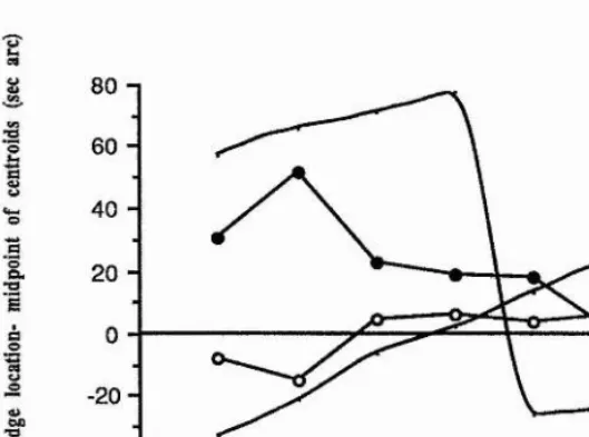
Another study of perceived spatial extent was conducted by Levi and Westheimer (1987), who determined whether variations in the luminance profile of a stimulus consisting of two bars influenced the perceived separation of the bars, and the precision with which separation could judged. Their stimulus was made up of seven unresolved lines, with an eighth added to one of the bars to alter the location of the centroid of the retinal intensity distribution for the bar. The location of the centroid of the intensity distribution did not affect thresholds for interval width discrimination but did affect the point of subjective equality (PSE) of interval width- and the perceived width of the interval was closely matched by the separation of the centroids of the retinal intensity distribution. This is similar to the data of Westheimer and McKee (1977a) for vernier acuity, in which they showed that vernier alignment for very similar stimuli depended on the centroid of the retinal intensity distribution. This suggests initially that the way in which spatial extent is assessed and relative location in a vernier task is measured have some similarities; it may be that the perceived width of an interval is determined by the location of the spatial primitives, but there is yet another source of information for interval width judgments which is not limited by contrast (unlike localising the centroids of zero-

bounded response distributions, for instance).

Levi and Westheimer (1987) also determined thresholds and points of subjective equality for stimuli composed of two bars with a lower contrast bar between them. This internal bar had no effect on threshold for discrimination of the separation of the outer bars (at contrasts up to 1/7 th that of the outer outer bars). However, the perceived width of the interval was dependent on the separation of the internal bar and the outer two bars; when the internal bars and outer bars were close, the interval between the outer two was seen as narrower. If the internal bar and the outer bars

(34)

were more widely separated, the interval width was overestimated. This result is directly analogous to findings of Badcock and Westheimer (1985a), who showed that a single flanking line alters the location of a target line in the same manner; ie. the lines are 'attracted' when close and 'repelled' when slightly further apart. This phenomenon (one aspect of spatial interference) is discussed at greater length in section 3.2.

The perceived relative location of a bright bar with an asymmetric orthoaxial contrast profile was determined by Toet, Smits, Nienhuis and Koenderink (1988), using interval bisection and vernier acuity tasks. For the bisection task, they found that the spatial primitive which best explained the results was dependent on the instructions given to the subject; if the subject was asked to attend to the width of the intervals between the three bars in the target, then zero-crossings in a hypothetical neural response (equivalent to a blurred second spatial derivative) were most appropriate. Without these explicit instructions being given, the relative localisation of the asymmetric bar was best explained by supposing that the visual system extracted either extrema or centroids from the hypothetical neural response to the stimulus. The significance of this result is unclear, since there have been no comparable reports of an interaction between spatial primitives and attentional, ie. top-down factors, which can be modulated by varying the instructions given.

1.6: Models of early vision

There have been many competing models of early vision. Exponents of the two broad theoretical alignments have been labelled "frequency freaks" and "feature creatures" (Krose, 1987). These two divisions reflect the differential emphasis on information in either the spatial frequency amplitude spectrum, or about the geometric (ie. spatial) properties of the stimuli. It would be fair to say that the feature creatures are (once again) in the ascendancy.

1.6.1: Frequencv based models

(35)

detectors, each with its own non-linearity (inspired by contrast discrimination experiments) and a noise source. Detecting a change in the spatial structure of the pattern takes place by analysing the change in response of the filter most sensitive to change in the pattern- ie. the filter which exhibits the greatest differential response between two patterns. The model predicts thresholds for relative localisation tasks, considering only the changes in the spatial frequency amplitude spectrum of patterns.

1.6.2: Wilson's model

One of the most influential models of early vision has been that of Wilson and Bergen (1979). Wilson's models have always been concerned with the energy in localised spatial frequency detectors and do not merit the 'hybrid' character that he claims for them. This statement is justified below. Wilson and Bergen's (1979) models of threshold spatial vision was derived from a re-analysis of data in a previous work by Wilson (1978); Wilson (1978) measured the influence of subthreshold flanking lines on a target line's detectability at different flanking distances, repeating this for two forms of temporal modulation ('sustained' and 'transient') as well as three different eccentricities. The line-spread function (LSF) for the system with a given set of parameters describes the sensitivity of the system as a function of the separation of the target and the subthreshold flanking lines. For lines with the same contrast polarity, the flanking lines facilitate detection when they are close to the target line, and inhibit detection when slightly further away, the inhibition effect diminishing at greater distances, giving a non-monotonic function relating sensitivity to flanking distance.

Wilson used the line-spread functions from this data set to estimate the filter profile and sensitivity of two bandpass filters which best explained the line detection data. This gave him a model for spatial contrast detection, which he used to predict thresholds for detecting Difference- of- Gaussian (DOG) patterns and cosine bars. The data were not well explained by the model predictions, with evidence of both lower and higher peak frequency bandpass filters contributing to the detection of these patterns.

Consequently, Wilson and Bergen (1979) modelled the data for detection of DOG patterns of different sizes with four filters, one higher and the other lower in peak frequency to the filters in Wilson's (1978) model. Wilson and Bergen's model is

32

(36)

based loosely upon Quick's (1974) vector magnitude model for detecting spatial patterns, in which the responses of independent detectors are combined by some magnitude function prior to detection; the magnitude function is given by

vector magnitude sum of ( R ) = [ Z ( Ri )p ] where R = { R^ ,R2 ,...Rn }•

In other words, the responses of a range of detectors are combined into a single sum, which depending on the value of p (the exponent) will range from an arithmetic mean (p=l) to peak detection (for large p). Wilson and Bergen fitted the DOG data from Wilson (1978) with four types of filter, each having different sensitivities, different space constants and different temporal response characteristics.

Responses of individual filters are computed by convolving the filter profile with the luminance profile of the stimulus, with the response being weighted by an amount which is proportional to the sensitivity of each detector. Whilst Wilson and Bergen's model has only four scales of filter, there are a larger number of filters pooled to derive the theoretical response of the system. To predict theoretical detection thresholds for the DOG patterns, they use five filters of each type, the centres of each of these being separated by 2.0 min arc.

The reason for incorporating units which are not centred under the stimulus is to improve the fit to the data- Wilson's approach is to start with the simplest possible model configuration to see if this can explain the data, and if it does not, add an extra mechanism and see how well this new configuration fits the data. The main point of Wilson's work is that a relatively small number of spatial filters generally provide adequate explanation of detection sensitivity.

(37)

necesssary to explain the threshold evelation data, within the limits imposed by experimental error.

Wilson and Bergen's model of detection was extended to cover discrimination tasks by Wilson and Gelb (1984), in their 'modified line-element' model of spatial discrimination, named by analogy with line-element models in colour vision. Six peak frequencies of filters were employed in Wilson and Gelb’s model, ranging in peak frequency from 0.8 to 16.0 c/deg. Filter sensitivities and bandwidths were estimated from the masking data of Wilson et al (1983). The response of each filter to the stimulus is computed by convolution of the pattern's luminance profile with the filter profile, the response is then weighted by the filter's sensitivity. Then the response is passed through a contrast transfer function, with each filter having a different transfer function. Response of each filter to the first pattern is then stored. The procedure is repeated when the second pattern is presented to the system.

The difference in response magnitude of each individual filter to the two patterns is then computed for each filter type; if we write the difference in magnitude of the i*^ filter response to the two patterns as dR^ and the vector of differences as dR

dR = { dRj, dR2, dRn) for n filters

then Wilson's model involves computing the vector magnitude sum for dR using Quick's (1974) formulation given above. The difference in response of each filter size to each pattern is computed for filters centred under the stimulus and for one filter either side of this centred filter. The model pools across these spatially offset filters, and therefore discards potential information about the spatial distribution of responses, taking only the magnitude of the difference in response in each filter to each of the two patterns. This model therefore does not merit being called a 'hybrid' model, since there is no information preserved about the spatial distribution of filter response, unlike models such as MIRAGE (Watt & Morgan, 1985) or Marr and Hildreth (1980).

In Wilson (1986), a two-dimensional extension of Wilson and Gelb's (1984) model is applied to a wide range of pattern acuity data; this model (Wilson, 1986) is identical in form to Wilson and Gelb's model, but incorporates orientation selective filters, and pooling across all orientations before a decision is made. Wilson (1986)

34

(38)

attempts to explain a wide range of data with a single model with very few free parameters. Wilson notes that his model is inappropriate or fails completely to explain performance on relative localisation tasks involving widely separated, relatively fine features (eg. separated by more than 1 deg). This is principally because it does not allow for activity in filters which are not spatially near neighbours as a source of information about relative location. It cannot do so, because information about the spatial location of filters is not preserved at all in Wilson's scheme and this seems to be its basic philosophy. Very low frequency filters would have to carry information about the relative location of widely separated features, lower than Wilson could find evidence for with his masking experiments.

Wilson's model has a very large 'null-space'; this is the equivalence class of patterns which Wilson's model fails to discriminate (Nielsen & Wandell, 1988). Given the representation that Wilson advocates does not have the property of uniqueness, there are many ways of mapping different patterns into the same point in Wilson's multidimensional filter response space. Additionally, there are many patterns which would be seen as perceptually identical which Wilson's model identifies as quite different. Since Wilson's model discards information about local image geometry, it is capable of making discriminations only when the spatial frequency amplitude spectra of patterns have a meaningful relationship to the changes in pattern which have to be identified.

(39)

discrimination, although a system that could analyse changes in the 'shape' of the amplitude spectrum (ie. the relative distribution of energy across spatial frequency) could deal with this situation. However, changes in the activity of any particular subset of filters would not give useful information about the intervals to be discriminated, which is contrary to simple models like Wilson's or Carlson and Klopfenstein's.

To eliminate the possibility that the system performs some more elaborate analysis of the frequency amplitude spectrum of each pattern, they determined interval thresholds for a target which consisted of four lines, which was compared with a two-line reference interval. The separation of the outer lines was randomly varied; the subjects had to discriminate the width of the innermost interval and the width of the two line reference interval. This manipulation will randomly perturb the 'shape' of the frequency amplitude spectra of the two patterns from trial to trial. They found that the random perturbation in flanking distance of the outer lines had not effect on threshold for the interval task. To explain this result, Wilson's model would have to conclude that the system can discover which filters carry most information about the change in interval width (rather than those which have the biggest differential response to the two patterns). Wilson (1986) mentions that a different strategy would be needed for this stimulus situation anyway, since the Wilson model would indicate that the two stimuli to be compared in this experiment are different in the first instance; but this seems to refute his own claim of having a unified theory of pattern discrimination.

1.6.3: Computational approaches : localising intensitv changes

This section describes some computational approaches to the detection of intensity changes in the image. The process of identifying and assigning location to intensity discontinuities is important as a means of data reduction, and may also be critically necessary for higher-level visual processes to work dependably. Conventionally, intensity changes are detected with differential operators. Differential operators are notoriously sensitive to noise, but we can overcome this by smoothing the image; also, since we do not know in advance how blurred an intensity change in the image will be, we may have to look at the filtered image on many spatial scales; generally, signal-to-noise ratios will differ for all edges in an image, and it is necessary to incorporate several different operators with different scales in to the scheme for detecting edges (the largest filters having good sensitivity

(40)

but poor localisation ability). Marr and Hildreth (1980) were the first to do this. Integrating the outputs of different scales of operators is a problem which has not yet been adequately solved.

Marr and Hildreth (1980) were also influential in proposing the use of Laplacian of a Gaussian function. Their model of edge localisation involved blurring the image with Gaussians of different space constants, and taking the Laplacian (the sum of the pure partial derivatives in orthogonal directions) of these blurred images. In practice, given the linearity of the convolution operator, we can combine these two steps into one convolution, by using an isotropic difference-of-Gaussians function, which for a centre-surround ratio of 1:1.6, gives a good engineering approximation to the Laplacian of a Gaussian. Marr and Hildreth's symbolic representation of edges consisted of a set of zero-crossing segments detected by operators with different spatial scales, along with the slope of the directional derivative perpendicular to each zero-crossing segment. Alternatively, since zeros are difficult to detect in a noisy system like the brain, they suggested that the location of zero-crossings could be estimated by interpolating between extrema of opposite sign in the filter output (Marr, Ullman & Poggio, 1979). The zero-crossing segments from the different spatial scales of filters were then combined into one representation by an algorithm based on the "spatial coincidence assumption"- if zero-crossings from filters adjacent in scale coincide, then this is enough to indicate the presence of an edge. Provided two filters that are reasonably separated in peak frequencies signal an edge, an edge primitive is represented in the 'primal sketch', a symbolic representation of intensity changes in the retinal image.

1.6.4: The optimal edge-finder