Analysis of Objectives Relationships in Multiobjective
Problems Using Trade-Off Region Maps
Rodrigo L. Pinheiro
ASAP Research Group School of Computer Science The University of Nottingham
[email protected]
Dario Landa-Silva
ASAP Research Group School of Computer Science The University of Nottingham
[email protected]
Jason Atkin
ASAP Research Group School of Computer Science The University of Nottingham
[email protected]
ABSTRACT
Understanding the relationships between objectives in many-objective optimisation problems is desirable in order to de-velop more effective algorithms. We propose a technique for the analysis and visualisation of complex relationships between many (three or more) objectives. This technique looks at conflicting, harmonious and independent objectives relationships from different perspectives. To do that, it uses correlation, trade-off regions maps and scatter-plots in a four step approach. We apply the proposed technique to a set of instances of the well-known multiobjective multidimensional knapsack problem. The experimental results show that with the proposed technique we can identify local and complex relationships between objectives, trade-offs not derived from pairwise relationships, gaps in the fitness landscape, and re-gions of interest. Such information can be used to tailor the development of algorithms.
Categories and Subject Descriptors
G.1.6 [Optimisation]; I.2.8 [Problem Solving, Control Methods, and Search]
Keywords
multiobjective fitness landscape analysis; trade-off region maps; fitness landscape visualisation
1.
INTRODUCTION
It is important to understand the relationships between objectives in multiobjective optimisation problems (MOPs) because this can help to tailor the search according to the multiobjective fitness landscape. This is particularly when tackling large real-world MOPs with many objectives (more than two). In the multiobjective optimisation literature, the focus is often on MOPs that exhibit strong conflict relation-ships between objectives as this is part of the motivation for applying multiobjective techniques. However, the conflict relationship between objectives could be local rather than
Permission to make digital or hard copies of all or part of this work for personal or classroom use is granted without fee provided that copies are not made or distributed for profit or commercial advantage and that copies bear this notice and the full citation on the first page. Copyrights for components of this work owned by others than the author(s) must be honored. Abstracting with credit is permitted. To copy otherwise, or republish, to post on servers or to redistribute to lists, requires prior specific permission and/or a fee. Request permissions from [email protected].
GECCO ’15, July 11 - 15, 2015, Madrid, Spain c
⃝2015 Copyright held by the owner/author(s). Publication rights licensed to ACM. ISBN 978-1-4503-3472-3/15/07. . . $15.00
DOI:http://dx.doi.org/10.1145/2739480.2754721
global. Aglobal conflict relationshipwould hold throughout most, if not all of, the search space. On the other hand, a local conflict relationship would hold in a restricted re-gion of the search space, e.g. the objectives could be in conflict early in the search but not conflicting later. This was discussed by Knowles and Corne [1] in the context of the multiobjective quadratic assignment problem. Castro-Gutierrez et al. [2] studied the objectives’ relationships in multiobjective vehicle routing problems.
As the number of objectives increases, composite relation-ships between objectives might emerge, i.e. relationships between objectives (conflicting or otherwise) that are not global but localised and more complex. Several techniques have been previously applied for the analysis and visualisa-tion of relavisualisa-tionships between objectives in MOPs. These in-clude parallel coordinates, scatter-plots (which both involve graphical representations), Kendall correlation [3] (a quant-itative metric), and statistical measures [4], among others. Purshouse and Fleming [5] discussed these techniques in their research into the relationships between objectives in MOPs. Other works that have used some of these techniques include Castro-Gutierrez et al. [2] on multiobjective vehicle routing problems, and Ishibuchi et al. [6] on many-objective problems with correlated objectives. One limitation of these techniques is that they are most suited to identify only pair-wise relationships between objectives.
multidimensional 0-1 knapsack problem [8, 9] are presented in Section 5. Our main observation is that different instances of the same problem may exhibit very different relationships between objectives. Finally, Section 6 concludes the paper.
2.
RELATED WORK
Better understanding of fitness landscapes has been bene-ficial in multiobjective combinatorial optimisation (MOCO) problems. For example, Garrett and Dasgupta [10] [11] ad-apted single-objective landscape analysis techniques (distri-bution of optima, fitness distance correlation, ruggedness, random walk analysis and analysis of the geometry of the solution space) for tailoring multiobjective evolutionary al-gorithms. They applied such techniques to quadratic as-signment and generalised asas-signment problems with two ob-jectives. They concluded that the performance of hybrid algorithms benefits from using knowledge of the fitness land-scape. Castro-Gutierrez et al. [2] used the objectives’ pair-wise dependency correlation analysis proposed by Purshouse and Fleming [5] to assess the conflicting nature of objectives in multiobjective vehicle routing problems.
Brownlee and Wright [12] proposed a visualisation tech-nique to evaluate the quality of a non-dominated set based on a ranking of the objectives. However, this technique may not be suitable for large solution sets as it is based on the in-dividual analysis of solutions. Other visualisation techniques include objective wheels, bar graphs and colour stacks as ex-plored by Anderson and Dror [13].
Verel et al. [14] adapted single-objective landscape ana-lysis techniques to set-based multiobjective problems with objective correlation. Later, Verel et al. [15] conducted a study on the landscape of local optima in such problems. Verel et al. [16] proposed to carry outa priori analysis of a problem by evaluating the problem size, its epistasis, the number of objectives and the correlation values between ob-jectives, to suggest the best way to tackle it. They concluded that, depending on the problem features, different types of algorithms (scalar or Pareto approach) and sizes of the solu-tion archive should be employed.
Walker et al. [17] reviewed different methods (scatter plots, parallel coordinates and heat maps) to visualise solution sets for many-objective problems. They also proposed two tech-niques: a data mining visualisation tool to plot a convex graph, and a new similarity measure of solutions to plot them in a two-dimensional space.
Giagkiozis and Fleming [18] proposed a technique to es-timate the Pareto front of a continuous optimisation prob-lem, and then use the estimated front to obtain values for the decision variables of interesting solutions. They pro-posed using a multiobjective algorithm to obtain an initial solution set, which is then used to calculate a projection matrix of the optimal Pareto set. They tested their tech-nique on convex benchmark problems.
Tusar and Filipic [19] presented a comprehensive survey and assessment on several visualisation techniques for many-objectives approximation sets. They also presented a visual-isation method that uses orthogonal projections of a section and applied it to four-dimensional approximation sets.
It is clear that understanding the fitness landscape of mul-tiobjective optimisation can help to develop better solution methods. It is also clear that the analysis and visualisa-tion of objectives’ relavisualisa-tionships, particularly in combinator-ial landscapes with many objectives, is a topic of interest for
0.2 0.4 0.6 0.8 0.2
0.4 0.6 0.8 1
Z1
[image:2.612.354.522.55.184.2]Z2
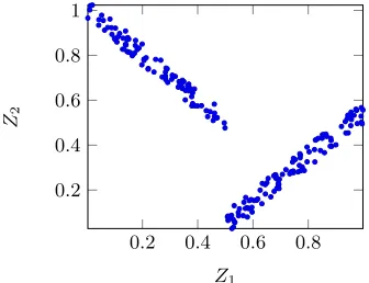
Figure 1: Example of complex relationship between two ob-jectivesZ1 andZ2 in a 3-objective optimisation problem.
researchers. The technique proposed in this paper seeks to make a contribution in this area.
3.
OBJECTIVES RELATIONSHIPS IN
MULTIOBJECTIVE OPTIMISATION
The focus of this research is to investigate the relation-ship between objectives in MOPs by analysing the non-dominated approximation set and its coverage of the solu-tion space. We use the concepts of conflict, harmony and independence between objectives as proposed by Purshouse and Fleming [5].Results from some existing techniques to assess the con-flicting nature of objectives can be deceiving. The literature includes studies of pairwise relationships between objectives [2, 6, 20]. However, analysis techniques such as Kendall correlation [3] only manage to identify global relationships between objectives. Figure 1 shows a Pareto-front between two maximisation objectives,Z1 andZ2, in a scenario with
three objectives (we omit the scatter-plots forZ3). Clearly,
when Z1 < 0.5, the objectives are conflicting while when
Z1 > 0.5 the objectives are harmonious. However, if the
number of solutions with Z1 lower than 0.5 is roughly the
same as the number of solutions with Z1 higher than 0.5,
simply applying the Kendall correlation technique would res-ult in a correlation value close to 0. The conclusion could be drawn that the objectives are independent, when in reality there may belocal relationships that could be exploited.
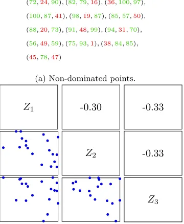
Some existing techniques might not reveal trade-offs which result fromcomposite relationships between two and more objectives. Figure 2a lists a set of non-dominated fitness vec-tors for three maximisation objectives and Figure 2b shows their scatter-plot matrix and correlation values. We can ob-serve that high values (51-100) appear simultaneously only in up to two of the three objectives. Two points in Figure 2a have only one good objective value. Four points are good for onlyZ1 andZ2. Three points are good for onlyZ1 and
Z3, and the remaining points are good for onlyZ2 andZ3.
No solution present has values higher than 50 for all three objectives simultaneously. The scatter plot and correlation values do not help us to appreciate the three-way trade-off. Likewise, we can see that the correlation values do not in-dicate any strong pairwise correlation.
(45,68,85),(6,63,99),(34,64,95), (28,100,48),(98,47,69),(48,62,79), (72,24,90),(82,79,16),(36,100,97), (100,87,41),(98,19,87),(85,57,50),
(88,20,73),(91,48,99),(94,31,70), (56,49,59),(75,93,1),(38,84,85), (45,78,47)
(a) Non-dominated points.
Z1 -0.30 -0.33
Z2 -0.33
Z3
[image:3.612.90.270.91.310.2](b) Scatter-plot matrix and correlation coefficients.
Figure 2: Three-way conflicting objectives
between objectives as well as interesting trade-offs in the fitness landscape.
4.
A FOUR STEPS ANALYSIS AND
VISUALISATION TECHNIQUE
We propose a four-step technique to analyse and visual-ise objectives relationships. It requires some knowledge of the problem domain (the desirable range of objective val-ues) and an approximation set of non-dominated solutions, which could be obtained using any multiobjective algorithm (MOA), such as those available in frameworks like JMetal [21] and ParadiseEO [22]. The quality of the approxima-tion set given may affect the conclusions from the analysis because inaccurate ranges and scatter plots could lead to in-accurate observations, thus combining the results from the application of a number of well-accepted MOAs may be wise. The scope of our technique is to aid the study of a sub-set of problem instances, to aid in tailoring an algorithm for solving other problem instances. Our aim in this work is to investigate the suitability of our technique, hence we test it on scenarios for which good algorithms are known. Although the approach requires some instances to be solved before-hand, the increased understanding of the problem should help in identifying the strengths and weaknesses of novel al-gorithms. Solution of these many-objectives problems are computationally expensive thus any help in tailoring fast techniques that can provide good-enough results has value, and this technique may allow a user to identify similarities between instances which could be exploited.
Each step in the proposed technique aggregates some in-formation about the relationship between objectives, the coverage of the feasible solution space and the trade-offs in the fitness landscape. The four steps are described here and
are illustrated by applying them to benchmark instances of the multiobjective multidimensional knapsack problem.
Step 1 – Global Pairwise Relationship Analysis:
First, the Kendall correlation values [3] are calculated, as in [5], to identify global pairwise relationships. Strongly con-flicting correlations (values < −0.5) immediately indicate that a trade-off surface exists, whilst strongly harmonious correlations (values>0.5) indicate that objectives could be aggregated or clustered. Correlation values showing that ob-jectives are independent indicate that the data is not glob-ally dependent, but do not imply the absence of local trade-offs in the fitness landscape. If independence is detected, the problem could be decomposed by separating the decision variables according to the objectives, to solve each object-ive (or groups of objectobject-ives) separately as such an approach provides improved performance [23].Step 2 – Objective Range Analysis:
Here, the range (difference between best and worst values) is calculated for each objective in the given approximation set. Then, using problem domain knowledge the objectives which are interesting for further exploration are identified. Ameaningful objectiveis an objective with a range which is large enough so that solutions can be classified into different quality categories regarding that objective value (e.g. good to bad, high to low, etc). Analogously, a non-meaningful objective is an objective with a range so small that the vari-ability in the solution quality regarding that objective is considered negligible, thus not worth exploring further.
One way to deal with non-meaningful objectives is to ig-nore them during the optimisation. It is possible that by op-timising the other objectives, the non-meaningful ones will present acceptable values within their small range anyway. Having a small range on the given approximation set does not mean that the range will be small across the entire solu-tion space. The non-meaningful objective could be removed, the MOA re-executed and the ranged recalculated for the ex-cluded objective. If the new solution set still exhibits only a small range for the excluded objective, it can be safely ig-nored. Another way to deal with non-meaningful objectives is to combine or cluster them [20].
Step 3 – Trade-off Regions Analysis:
We apply a quantitative method, namely Karnaugh maps [7], to classify the solution space into regions to help with the identification of trade-offs and the complex relationships between objectives. A Karnaugh map is a method for simpli-fying boolean algebra expressions using a truth table. The map has 2i cells where iis the number of variables. The cells are labelled with binary numbers following the Grey code, meaning that any two adjacent cells differ in one bit. Hence, in a three variable scenario, the cells adjacent to cell 0 (0002) are cells 1(0012), 2(0102) and 4(1002). Karnaugh
maps make it easy to visualise patterns that are used to group boolean variables.
In this step, for each objectiveZi where (i= 1,2, . . . m),
we define a thresholdtisuch that values aboveti
(maximisa-tion problem) are considered good or acceptable, and values belowti are considered inadequate. Thesetican be set
solution as good (↑) or bad (↓). Finally, we draw aregion map similarly to a Karnaugh map, but showing the count of solutions in each region rather than 0-1 output variables, and using solutions classifications (labelled↑and↓) instead of the input variable values. The map is built with 2m re-gions such that each region represents a single combination of good and/or bad objectives. We number the regionsrk
using a binary encoding such that the least significant digit representsZ1and the most significant digit isZm,↑= 0 and
↓= 1. For instance, the region Z3↓, Z2↑ and Z1↓, would be
regionr5, since binary 1012 is 5.
Z2↑ Z2↓ Z3↑ r0 r1 r3 r2
Z3↓ r4 r5 r7 r6
Z1↑ Z1↓ Z1↑
(a) Three Objectives
Z2↑ Z2↓
r0 r1 r3 r2 Z3↑
Z4↑ r
4 r5 r7 r6
r12 r13 r15 r14 Z ↓ 3
Z4↓ r
8 r9 r11 r10 Z3↑
Z1↑ Z1↓ Z↑1
(b) Four Objectives
Z5↑ Z5↓
Z2↑ Z2↓ Z2↑ Z2↓
r0 r1 r3 r2 r16 r17 r19 r18 Z3↑
Z4↑
r4 r5 r7 r6 r20 r21 r23 r22
r12 r13 r15 r14 r28 r29 r31 r30 Z
↓ 3
Z4↓
r8 r9 r11 r10 r24 r25 r27 r26 Z3↑
Z1↑ Z1↓ Z1↑ Z1↓ Z1↑
[image:4.612.54.293.181.422.2](c) Five Objectives
Figure 3: Region map schematics.
Figure 3 presents the region map schematics for 3, 4 and 5 objectives. Each region is identified with therk. Regions
with the same number of good solutions are highlighted with the same shade of grey in such a way that lighter tones represents a higher number of good solutions while darker tones represents fewer good solutions.
The main advantage of the region map is that we can easily identify which objectives simultaneously present good values and the existence of trade-offs. If the region r0 is
not empty, then we have solutions with acceptable values in all objectives, meaning that the problem could potentially be tackled with single-objective algorithms. A range ana-lysis on the solutions in this region could provide additional information on which approach is appropriate. On the con-trary, when most solutions fall into regionr2m−1, it means
that the thresholds may have been set too high and should be lowered for more accurate results. When there are no solutions inr0, but there are solutions scattered across the
regions, there are trade-offs and the map can be used to visualise them.
Step 4 – Multiobjective Scatter-plot Analysis:
The last step is an analysis using scatter plots. First, for each instance we normalise the values of all objectives. Then, we select an objective and draw a scatter plot of all
remain-ing objectives against the selected objective. Finally, we can combine all scatter plots into a single one. By visually inspecting this combined graph we can identify local rela-tionships (conflicts and harmony), interesting patterns, gaps in the solution space, and well-spread trade-offs or isolated regions. This information can help us to tailor a solution algorithm by directing the search towards the regions of in-terest. When the landscape of the solution space is consist-ent throughout all instances analysed in this way, we could have a clearer idea of what type of solutions to expect when solving unseen instances.
When picking an objective for this process, it is prefer-able to select one that has a wider range of values rather than being concentrated in only a small range, otherwise the resulting graph may be more difficult to read. It may be interesting to test different objectives in order to spot which provide more useful information, or, if multiple objectives provide different insights, all of them could be considered instead of only one.
The next section presents experimental results from ap-plying the proposed analysis and visualisation technique to five sets of benchmark instances of the multiobjective mul-tidimensional knapsack problem.
5.
SAMPLE ANALYSIS
In order to illustrate the analysis technique we apply it to different scenarios of the multiobjective multidimensional knapsack problem (MOMKP) [8]. We aim to show that within the same problem, the proposed technique can identify multiple scenarios with distinct multiobjective natures.
In the MOMKP, we haven items (i= 1, . . . , n) with m weightswji (j = 1, . . . , m) and p profits c
i
k (k = 1, . . . , p).
A set of items must be selected to maximise the p profits while not exceeding the capacitiesWjof the knapsack. This
problem can be formulated as follows:
maximise
n ∑
i=1
cikxi k= 1, . . . , p
subject to
n ∑
i=1
wjixi≤Wj j= 1, . . . , m
xi∈0,1 i= 1, . . . , n
We considered five MOMKP datasets, each with five in-stances, all with m = 4, p = 4, n = 1000 and Wj =
50000. The first four datasets were generated following the guidelines in Bazgan et al. [9] and are as follows:
• Set A: Independent random instances wherewik ∈N
[1,1000] andcik∈N[1,1000].
• Set B: Uncorrelated harmonious instances where
wik∈N[1,1000],ci1∈N[1,1000] andcik∈N [max{cik−1
−100,1}, min{cik−1+ 100,1000}] fork= (2,3,4).
• Set C: Uncorrelated conflicting instances wherewki ∈N
[1,1000],ci1∈N[1,1000] andcki ∈N [max{900−cik−1,
1}, min{1100−ci
k−1,1000}] fork= (2,3,4).
• Set D: Correlated conflicting instances wherewi1∈N
[max{900− |ci1−ci4|,1},min{1100− |ci1−ci4|,1000}],
wi
k∈N [max{900− |cik−cik−1|,1}, min{1100− |cik−
cik−1|,1000}], c i
1 ∈N [1,1000] and cik ∈N [max{900−
cik−1,1},min{1100−c i
[image:4.612.346.529.437.506.2]SetA contains only independent objectives. In setB all objectives are harmonious. Set C contains three pairs of conflicting objectives, (Z2, Z1), (Z3, Z2) and (Z3, Z4), while
the weights are uncorrelated. SetDhas conflicting object-ives, as setC, but the weights are correlated to the objective values. The fifth setXwas generated using data from a real-world home health-care scheduling problem.
Set A A1 A2 A3 A4 A5 Mean
Z1-Z2 -0.15 -0.33 -0.21 -0.39 -0.49 -0.314
Z1-Z3 -0.02 0.09 -0.43 -0.34 0.11 -0.118
Z1-Z4 -0.21 0.09 -0.18 0.20 0.07 -0.006
Z2-Z3 -0.30 -0.37 0.17 0.01 -0.42 -0.182
Z2-Z4 0.06 -0.22 -0.17 -0.41 -0.09 -0.166
Z3-Z4 -0.25 -0.20 -0.22 -0.26 0.19 -0.148
Set C C1 C2 C3 C4 C5 Mean
Z1-Z2 -0.96 -0.97 -0.98 -0.98 -0.98 -0.974
Z1-Z3 0.93 0.95 0.95 0.96 0.96 0.950
Z1-Z4 -0.93 -0.92 -0.92 -0.97 -0.95 -0.938
Z2-Z3 -0.96 -0.96 -0.97 -0.97 -0.96 -0.964
Z2-Z4 0.95 0.92 0.93 0.96 0.94 0.940
Z3-Z4 -0.98 -0.94 -0.95 -0.97 -0.97 -0.962
Set D D1 D2 D3 D4 D5 Mean
Z1-Z2 -0.92 -0.92 -0.94 -0.94 -0.94 -0.932
Z1-Z3 0.88 0.84 0.88 0.87 0.87 0.868
Z1-Z4 -0.84 -0.84 -0.87 -0.87 -0.87 -0.858
Z2-Z3 -0.87 0.90 -0.91 -0.90 -0.90 -0.896
Z2-Z4 0.82 0.86 0.87 0.87 0.87 0.858
Z3-Z4 -0.92 -0.93 -0.93 0.92 -0.92 -0.924
Set X X1 X2 X3 X4 X5 Mean
Z1-Z2 -0.26 -0.29 -0.13 -0.24 -0.32 -0.248
Z1-Z3 -0.13 -0.24 -0.27 -0.25 -0.27 -0.232
Z1-Z4 -0.29 -0.12 -0.29 -0.21 -0.07 -0.196
Z2-Z3 -0.25 -0.13 -0.26 -0.23 -0.19 -0.212
Z2-Z4 -0.13 -0.28 -0.22 -0.11 -0.27 -0.202
[image:5.612.324.540.51.611.2]Z3-Z4 -0.24 -0.23 -0.14 -0.21 -0.18 -0.200
Table 1: Results for the pairwise relationship analysis (1.0 is completely harmonious, -1.0 is completely conflicting).
For each instance we run a single-objective genetic al-gorithm on each objective alone, then both NSGAII [24] and MOEA/D [25] algorithms on each pair and triple of ob-jectives. We then combined all the obtained non-dominated solutions into an archive. We randomly drew from the archive half of the individuals for the initial population and the other half were randomly generated. We performed three runs for the MOEA/D and three runs for the NSGA-II with all ob-jectives. The approximation non-dominated set was formed with all non-dominated solutions which were found in the process. Both NSGAII and MOEA/D used a population of 200 individuals, binary tournament selection and half uni-form crossover [26] for 1500000 function evaluations. Over-all, we obtained non-dominated sets with approximately 900 solutions for setA, 3 for setB, 550 for setC, 1500 for set
Dand 2500 solutions for setX.
Only a few non-dominated solutions were found for set
B, the objectives there are strongly harmonious. Therefore, when maximising one of the objectives, the other object-ives are also maximised. The data is therefore not enough for some of the analysis steps. However, the results are presented for completeness and illustrate that the number
Set A A1 A2 A3 A4 A5 Mean
Z1
Max 105269 105591 98845 109048 98562 103463.0 Min 81507 84910 72393 82400 78259 79893.8 Range 22.6% 19.6% 26.8% 24.4% 20.6% 22.8%
Z2
Max 105565 102067 101879 107485 106290 104657.2 Min 84618 78862 75194 78073 82345 79818.4 Range 19.8% 22.7% 26.2% 27.4% 22.5% 23.7%
Z3
Max 100267 105755 106024 110554 102331 104986.2 Min 76363 80682 78207 82257 77085 78918.8 Range 23.8% 23.7% 26.2% 25.6% 24.7% 24.8%
Z4
Max 107607 110827 105888 103686 106472 16895.4 Min 84932 88405 75817 76770 86274 82439.6 Range 21.1% 20.2% 28.4% 26.0% 19.0% 22.9%
Set B B1 B2 B3 B4 B5 Mean
Z1
Max 103713 n/a 104141 111900 n/a 106584.7 Min 102748 n/a 104107 111622 n/a 106159.0 Range 0.9% n/a 0.1% 0.2% n/a 0.4%
Z2
Max 104952 n/a 107233 113620 n/a 108601.7 Min 104410 n/a 106638 113496 n/a 108181.3 Range 0.5% n/a 0.6% 0.1% n/a 0.4%
Z3
Max 106633 n/a 109010 113821 n/a 109821.3 Min 106274 n/a 108175 113479 n/a 109309.3 Range 0.3% n/a 0.8% 0.3% n/a 0.5%
Z4
Max 107347 n/a 108361 113926 n/a 109878.0 Min 107025 n/a 107324 113663 n/a 109337.3 Range 0.3% n/a 1.0% 0.2% n/a 0.5%
Set C C1 C2 C3 C4 C5 Mean
Z1
Max 109142 105928 114773 115084 112290 111443.4 Min 34911 33631 35449 35317 33157 34493.0 Range 68.0% 68.3% 69.1% 69.3% 70.5% 69.0%
Z2
Max 111124 109863 110290 114339 112559 111635.0 Min 37928 36764 33189 30491 32431 34160.6 Range 65.9% 66.5% 69.9% 73.3% 71.2% 69.4%
Z3
Max 109775 104817 113400 115214 112467 111134.6 Min 35859 33066 35326 35508 33004 34552.6 Range 67.3% 68.5% 68.8% 69.2% 70.2% 68.9%
Z4
Max 109569 108055 109242 113106 113391 110272.6 Min 38774 37107 34277 32074 34062 35258.8 Range 64.6% 65.7% 68.6% 71.6% 69.4% 68.0%
Set D D1 D2 D3 D4 D5 Mean
Z1
Max 186945 190209 188157 170337 179792 183088.0 Min 58152 65554 69709 53810 64747 62394.4 Range 68.9% 65.5% 63.0% 68.4% 64.0% 65.9%
Z2
Max 180305 188813 197847 183889 191691 188509.0 Min 64198 58680 68608 55859 63604 62189.8 Range 64.4% 68.9% 65.3% 69.6% 66.8% 67.0%
Z3
Max 185349 189131 187175 169153 180283 182218.2 Min 56697 63717 68430 52449 67272 61713.0 Range 69.4% 66.3% 63.4% 69.0% 62.7% 66.1%
Z4
Max 182878 188835 196048 182326 190441 188105.6 Min 66673 61884 70145 59158 66344 64840.8 Range 63.5% 67.2% 64.2% 67.6% 65.2% 65.5%
Set X X1 X2 X3 X4 X5 Mean
Z1
Max 29105 30825 29173 29906 30536 29909.0 Min 4930 3703 5317 4685 4429 4612.8 Range 83.1% 88.0% 81.8% 84.3% 85.5% 84.6%
Z2
Max 28885 30180 29314 28990 31422 29758.2 Min 4706 4506 5024 4027 4190 4490.6 Range 83.7% 85.1% 82.9% 86.1% 86.7% 84.9%
Z3
Max 299949 29488 28154 31445 30055 29818.2 Min 4096 4288 4298 4652 4102 4287.2 Range 86.3% 85.5% 84.7% 85.2% 86.4% 85.6%
Z4
[image:5.612.70.273.135.448.2]Max 30040 30478 30063 31103 29206 30178.0 Min 5075 3749 3673 4334 4563 4278.8 Range 83.1% 87.7% 87.8% 86.1% 84.4% 85.8%
Table 2: Results for the objective ranges analysis.
of solutions obtained can have a major impact on the ana-lysis and that, it is important to have a comprehensive set, with enough well-spread solutions.
5.1
Application of the Proposed Technique
coeffi-Z2↑ Z ↓ 2
01.2% 05.9% 07.9% 06.3% Z↑3
Z↑4 04.0% 06.5% 07.2% 08.6%
4.7% 11.2% 00.5% 08.0% Z
↓ 3
Z↓4 02.8% 06.7% 08.7% 10.0% Z↑ 3
Z1↑ Z ↓
1 Z
↑ 1
(a) Set A
Z2↑ Z2↓
45.0% 10.0% 11.7% 00.0% Z3↑
Z4↑ 00.0% 00.0% 00.0% 00.0%
13.3% 00.0% 00.0% 15.0% Z3↓
Z4↓ 00.0% 00.0% 05.0% 00.0% Z↑ 3
Z↑1 Z1↓ Z↑1
(b) Set B
Z2↑ Z2↓
00.0% 00.2% 00.3% 00.6% Z3↑
Z4↑ 00.0% 49.9% 01.9% 00.3%
00.0% 00.9% 00.8% 00.4% Z
↓ 3
Z4↓ 00.0% 00.2% 00.8% 43.5% Z↑ 3
Z↑1 Z1↓ Z↑1
(c) Set C
Z2↑ Z2↓
00.0% 00.0% 00.0% 00.0% Z3↑
Z4↑ 00.0% 55.6% 04.7% 00.0%
00.0% 04.4% 09.9% 01.8% Z3↓
Z4↓ 00.0% 00.0% 01.0% 22.6% Z↑ 3
Z↑1 Z1↓ Z↑1
(d) Set D
Z2↑ Z2↓
00.0% 00.0% 05.9% 00.0% Z3↑
Z4↑ 00.0% 06.2% 10.0% 05.9%
07.9% 15.4% 04.7% 15.0% Z3↓
Z4↓ 00.0% 07.1% 15.4% 06.4% Z↑ 3
Z↑1 Z1↓ Z↑1
[image:6.612.101.241.51.388.2](e) Set X
Table 3: Results for the trade-off regions analysis.
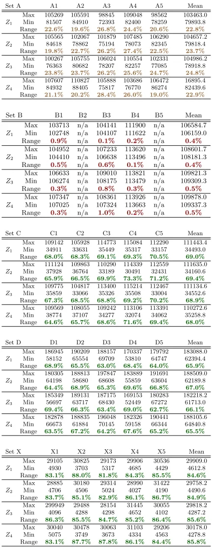
cient values for setBare not provided for the reason given above. The table presents the individual pairwise correla-tion value for each combinacorrela-tion of objectives. As expected for fully independent objectives, set A has values close to 0. The values for sets C and D are also predictably close to either 1 or−1 indicating global conflicting or harmoni-ous relationships. SetX has values similar toA– they do not reveal a strong global relationship between objectives as they are closer to 0 than to 1 or−1. Also, in set X it is not possible to decompose the decision variables according to the objectives, as every item has all weights and values above zero.
Step 2 - Objective Range Analysis. The results for this step are in Table 2. Considering setB, it can be seen, that the set presents small ranges of less than 0.3% on av-erage. In this dataset all objectives are harmonious and the solutions found are all located in a small region of the solu-tion space. These few solusolu-tions dominated all other solusolu-tions explored. Both setsCandDpresent similar results to each other with large ranges for each objective (over 60%). This is expected since these are instances with conflicting object-ives and present global trade-offs. The large ranges mean that while we have solutions with good values for a given objective, at least one other objective has poor value.
Finally, we highlight that while the global pairwise re-lationship analysis (step 1) hinted that setsA andX were similar, the difference between them now becomes clear with
the results from step 2. In set A, each objective range is around 24.0% of the maximum value – the smallest ranges excluding the harmonious instances – whilst in set X the ranges go up to 84.9%, the largest range found. Thus, we can see that the ranges for setX are closer to those for set
D, a conflicting scenario with global trade-offs.
Step 3 - Trade-Off Regions Analysis.The results for this step are in Table 3. For each instance we computed the number of solutions in each region and the map shows the average percentage for each set. We set the range threshold to 1% above the mean value found for each objective, thus considering a value slightly above the average to be good. We can observe that on setA the front is well distributed as we have solutions in all regions, scattered throughout the solution space, as a result of the independent objectives. Additionally, note that we have solutions both in r0 and
r15. This is due to the map presenting the combined results
for all five instances in that set, and in some instances we have solutions inr0 only and in other instances inr15only.
In setsC and D we clearly identify the global relation-ships. There are no solutions with good values in all object-ives and most instances present no solution with good values in three objectives. The majority of the solutions are situ-ated whereZ1 andZ3alone have good values and whereZ2
andZ4alone have good values, as these are the harmonious
pairs. Additionally, we can observe that almost no solutions are present in conflicting areas. For instance, whereZ1 and
Z2present good values simultaneously. Moreover, solutions
in conflicting areas should be close to the chosen threshold. The setX does not contain solutions in r0 and there are
no solutions in regions r1, r2, r4 and r8, meaning that no
high values can be simultaneously found for three or more objectives. We can find good values simultaneously only for up to two objectives. The map for setX resembles the ones for sets C andD in the sense that we can clearly see that there are several regions without solutions. Thus, we have trade-offs to present to the decision-maker. This means that the decision-maker has to choose between up to two good ob-jective values to the detriment of the remaining obob-jectives, since all of the regions containing solutions have at most two simultaneously good values.
Step 4 - Multiobjective Scatter Plot Analysis.This analysis was performed for each instance and Figure 4 presents the results for all instances of each set combined. We can see in Figure 4a that although instances in datasetAare com-pletely random, all of them show similar landscapes with a high concentration of solutions towards the (1,1) corner. Moreover, no local relationships can be identified, which is expected as the data is completely random.
On setsC andDwe can clearly see the trade-off regions. Also, there is a noticeable gap in the solution space when
Z1 is in the range from 0 to 0.5 and when the remaining
objectives are in the range from 0 to 0.4, approximately. Moreover, the landscape of the solution space appears to be similar for all instances of each of the setsC andD.
Since the data was uniformly generated (these gaps are unlikely to arise from the data itself) and could represent limitations in the solution algorithms, indicating that they did not explore the entire front. It is well known that the performance of some MOEAs is limited when the number of objectives is more than three [27].
(a) Set A (b) Set B (c) Set C (d) Set D (e) Set X
Figure 4: Results for the trade-off regions analysis.
noticing is that there is a lack of solutions with values within [0.85,1]. Again, this is due to limitations of the solution al-gorithms. However, we can see that the size of the gap is small, confirming that instances with strongly conflict-ing objectives present a bigger challenge to the algorithms. We can also identify several local relationships. When Z1
ranges from 0.5 to 0.8, the three remaining objectives sim-ultaneously conflict and harmonise. Knowing that only two simultaneous objectives present high values (from the region map analysis), we can conclude that wheneverZ1increases,
only one of the other objectives simultaneously increases too.
5.2
Discussion
With the proposed analysis and visualisation technique, we can better understand the multiobjective nature of the problem instances considered. Looking at only the correla-tion coefficients, we could conclude that: setsA andX do not present interesting multiobjective traits, that setB is inconclusive and that setsC andD present conflicting and harmonious objectives. However, by applying our analysis and visualisation technique we can reach a more compre-hensive understanding of these instance sets.
As fully random instances, datasetAdoes not present rel-evant global or local pairwise relationships according to the global pairwise analysis (step 1) and the multiobjective scat-ter plot analysis (step 4). Additionally, the objective range analysis (step 2) shows that even though there is a large set of non-dominated solutions, these are concentrated in a reasonably small area of the search space. For this dataset we can use the information from the trade-off region maps to interact with the decision-maker to identify which regions are of more interest and then use single-objective optimisa-tion algorithms to find soluoptimisa-tions in that region. Since we have solutions in all of the regions of the map, any objective vector could provide an adequate solution.
SetB presents a completely harmonious case and by ana-lysing the ranges and bearing in mind that the algorithms found just a handful of solutions, we can assume that a single-objective algorithm aiming to maximise any of the objectives could provide a reasonable good solution.
SetsC andDpresent similar scenarios, hence the correl-ation between weights and coefficients does not impact on the nature of the problem. The entire solution set repres-ents a huge trade-off. We also notice that the algorithms found it very difficult to expand along the front and that they mainly explored the region surrounding the intersec-tion of the trade-off. Nonetheless, by perceiving that all in-stances in these sets have similar landscapes and by knowing the approximate boundaries of each objective (by applying
single-objective algorithms to each objective alone), we can estimate the landscape of solutions for other instances in those sets. Therefore, we could direct the search to the re-gions of interest after presenting the expected trade-offs to the decision-maker. However, if it is imperative to use an a posteriori approach, the global pairwise analysis and the scatter plots provide sufficient information to make feasible the grouping of harmonious objectives.
Finally, setX presents a quite different picture. By only evaluating the global pairwise analysis (step 1) we conclude that there is no strong pairwise relationship between ob-jectives. However, the objectives range analysis (step 2) shows that in fact we have non-dominated solutions that vary greatly in quality. This is an indication of the exist-ence of trade-offs (as we can see by comparing this set with setsCandD). The trade-off region analysis (step 3) showed the existence of overall trade-offs as it is not possible to have solutions with good values in more than two objectives sim-ultaneously. Finally, the multiobjective scatter plot analysis (step4) identified local relationships between objectives and gaps in the solution space, pointing to the existence of local conflicts. Therefore, instances in dataset X exhibit a dis-tinctive multiobjective nature perhaps with interesting op-tions for a decision-maker. A sound possibility to tackle this problem would be to use the region map to identify the re-gions of interest and then locate those rere-gions in the scatter plot. In case a selected region contains a local conflict, we can use the algorithm proposed by [1] to reach the trade-off front and then expand through it.
6.
CONCLUSION
We proposed a technique that uses correlation, trade-off region maps and scatter-plots as tools for the analysis and visualisation of objectives’ relationships in multiobject-ive optimisation problems. The technique consists of four steps: 1) evaluate the global correlation values, 2) compute the range of values for all objectives, 3) compute the distri-bution of solutions in the different trade-off regions, and 4) conduct a scatter-plot analysis of the objectives.
visualisa-tion technique could be used to better understand the fitness landscape of the problem in hand.
Future work includes applying the proposed technique to other optimisation problems to validate further. It is also important to study the impact that the initial approximation set provided has on the accuracy of the analysis. Finally, we intend to investigate how the components of this technique, such as the trade-off region map, could be employed during the optimisation process for a many-objectives algorithm, to direct the search towards regions of interest.
7.
REFERENCES
[1] J. Knowles and D. Corne. Towards Landscape Analyses to Inform the Design of Hybrid Local Search for the Multiobjective Quadratic Assignment Problem. InSoft Computing Systems: Design, Management and Applications, pages 271–279, Amsterdam, 2002. [2] J. Castro-Gutierrez, D. Landa-Silva, and
J. Moreno Perez. Nature of real-world multi-objective vehicle routing with evolutionary algorithms. In Systems, Man, and Cybernetics (SMC), 2011 IEEE International Conference on, pages 257–264, 2011. [3] M. G. Kendall. A new measure of rank correlation.
Biometrika, 30(1/2):81–93, 1938.
[4] M. Khabzaoui, C. Dhaenens, and E.-G. Talbi. A multicriteria genetic algorithm to analyze DNA microarray data. InEvolutionary Computation (CEC), IEEE Congress on, pages 1874–1881, 2004. [5] R. C. Purshouse and P. J. Fleming. Conflict,
harmony, and independence: Relationships in evolutionary multi-criterion optimisation. In Evolutionary Multi-Criterion Optimization, volume 2632 ofLNCS, pages 16–30. 2003.
[6] H. Ishibuchi, N. Akedo, H. Ohyanagi, and Y. Nojima. Behavior of EMO algorithms on many-objective optimization problems with correlated objectives. In Evolutionary Computation (CEC), 2011 IEEE Congress on, pages 1465–1472, June 2011. [7] M. Karnaugh. The Map Method for Synthesis of
Combinational Logic Circuits. Trans. AIEE. pt. I, 72 (9):593–599, 1953.
[8] T. Lust and J. Teghem. The multiobjective
multidimensional knapsack problem: a survey and a new approach. CoRR, abs/1007.4063, 2010.
[9] C. Bazgan, H. Hugot, and D. Vanderpooten. An efficient implementation for the 0-1 multi-objective knapsack problem. InExperimental Algorithms, volume 4525 ofLNCS, pages 406–419. 2007. [10] D. Garrett and D. Dasgupta. Multiobjective
landscape analysis and the generalized assignment problem. volume 5313 ofLNCS, pages 110–124. 2008. [11] J. D. Garrett. Multiobjective Fitness Landscape
Analysis and the Design of Effective Memetic Algorithms. PhD thesis, Memphis, TN, USA, 2008. [12] A.r E.I. Brownlee and J. A. Wright. Solution analysis
in multi-objective optimization. InFirst Building Simulation and Optimization Conference, Loughborough, UK, 2012.
[13] R. K. Anderson and M. Dror. An interactive graphic presentation for multiobjective linear programming.
Applied mathematics and computation, 123:229–248, 2001.
[14] S. Verel, A. Liefooghe, and C. Dhaenens. Set-based multiobjective fitness landscapes: A preliminary study. InProceedings of the 13th Annual Conference on Genetic and Evolutionary Computation, GECCO ’11, pages 769–776, New York, NY, USA, 2011. [15] S. Verel, A. Liefooghe, L. Jourdan, and C. Dhaenens.
Pareto local optima of multiobjective NK-landscapes with correlated objectives. InEvolutionary
Computation in Combinatorial Optimization, volume 6622 ofLNCS, pages 226–237. 2011.
[16] S. Verel, A. Liefooghe, L. Jourdan, and C. Dhaenens. On the structure of multiobjective combinatorial search space: MNK-landscapes with correlated objectives. European Journal of Operational Research, 227(2):331 – 342, 2013.
[17] D. J. Walker, R. M. Everson, and J. E. Fieldsend. Visualizing mutually nondominating solution sets in many-objective optimization. Evolutionary
Computation, IEEE Transactions on, 17(2):165–184, 2013.
[18] I. Giagkiozis and P.J. Fleming. Pareto front estimation for decision making. Evolutionary Computation, MIT Press, Apr 2014.
[19] T. Tusar and B. Filipic. Visualization of pareto front approximations in evolutionary multiobjective optimization: A critical review and the prosection method. Evolutionary Computation, IEEE Transactions on, 19(2):225–245, April 2015. ISSN 1089-778X. .
[20] X. Guo, Y. Wang, and X. Wang. Using objective clustering for solving many-objective optimization problems. Mathematical Problems in Engineering, 2013.
[21] J. J. Durillo and A. J. Nebro. jMetal: A java
framework for multi-objective optimization. Advances in Engineering Software, 42:760–771, 2011.
[22] S. Cahon, N. Melab, and E.G. Talbi. ParadisEO: a framework for the reusable design of parallel and distributed metaheuristics. Journal of heuristics, 10: 357–380, 2004.
[23] R. C. Purshouse and P. J. Fleming. An adaptive divide-and-conquer methodology for evolutionary multi-criterion optimisation. InEvolutionary Multi-Criterion Optimization, volume 2632 ofLNCS, pages 133–147. 2003.
[24] K. Deb, A. Pratap, S. Agarwal, and T. Meyarivan. A fast and elitist multiobjective genetic algorithm: NSGA-II. Evolutionary Computation, IEEE Transactions on, 6(2):182–197, 2002.
[25] Q. Zhang and H. Li. MOEA/D: A multiobjective evolutionary algorithm based on decomposition. Evolutionary Computation, IEEE Transactions on, 11 (6):712–731, 2007.
[26] L. J. Eshelman. The chc adaptive search algorithm: How to have safe search when engaging in
nontraditional genetic recombination. InFOGA’90, pages 265–283, 1990.