Development of a statistical crop model to explain the relationship between seed yield and phenotypic diversity within the Brassica napus Genepool

agronomy

Article

Development of a Statistical Crop Model to Explain

the Relationship between Seed Yield and Phenotypic

Diversity within the

Brassica napus

Genepool

Emma J. Bennett1,†, Christopher J. Brignell2,†, Pierre W. C. Carion3, Samantha M. Cook3, Peter J. Eastmond3_{, Graham R. Teakle}4_{, John P. Hammond}5_{, Clare Love}6_{, Graham J. King}7_, Jeremy A. Roberts8and Carol Wagstaff1,*

1 _{Department of Food and Nutritional Sciences and Centre for Food Security, University of Reading,}

Whiteknights, PO Box 226, Reading, Berkshire RG6 6AP, UK; e.j.bennett@reading.ac.uk

2 _{School of Mathematical Sciences, University of Nottingham, University Park, Nottingham NG7 2RD, UK;}

Chris.Brignell@nottingham.ac.uk

3 _{Rothamsted Research, Harpenden, Hertfordshire AL5 2JQ, UK; pierre.carion@rothamsted.ac.uk (P.W.C.C.);}

sam.cook@rothamsted.ac.uk (S.M.C.); peter.eastmond@rothamsted.ac.uk (P.J.E.)

4 _{Warwick Crop Centre, University of Warwick, Wellesbourne CV35 9EF, UK; graham.teakle@warwick.ac.uk} 5 _{School of Agriculture, Policy and Development and Centre for Food Security, University of Reading,}

Earley Gate, Whiteknights Road, PO Box 237, Reading RG6 6AR, UK; j.p.hammond@reading.ac.uk

6 _{Rothamsted Research, Harpenden, Hertfordshire AL5 2JQ, UK; clare.love@mcri.edu.au}

7 _{Southern Cross Plant Science, Southern Cross University, PO Box 157, Lismore, NSW 2480, Australia;}

Graham.King@scu.edu.au

8 _{Office of the Vice-Chancellor, 18 Portland Villas, University of Plymouth, Plymouth, Devon PL4 8AA, UK;}

jerry.roberts@plymouth.ac.uk

* Correspondence: c.wagstaff@reading.ac.uk; Tel.: +44-118-378-5362 † These authors contributed equally to the work.

Academic Editor: Karin Krupinska

Received: 30 March 2017; Accepted: 19 April 2017; Published: 22 April 2017

Abstract:Plants are extremely versatile organisms that respond to the environment in which they find themselves, but a large part of their development is under genetic regulation. The links between developmental parameters and yield are poorly understood in oilseed rape; understanding this relationship will help growers to predict their yields more accurately and breeders to focus on traits that may lead to yield improvements. To determine the relationship between seed yield and other agronomic traits, we investigated the natural variation that already exists with regards to resource allocation in 37 lines of the crop species Brassica napus. Over 130 different traits were assessed; they included seed yield parameters, seed composition, leaf mineral analysis, rates of pod and leaf senescence and plant architecture traits. A stepwise regression analysis was used to model statistically the measured traits with seed yield per plant. Above-ground biomass and protein content together accounted for 94.36% of the recorded variation. The primary raceme area, which was highly correlated with yield parameters (0.65), provides an early indicator of potential yield. The pod and leaf photosynthetic and senescence parameters measured had only a limited influence on seed yield and were not correlated with each other, indicating that reproductive development is not necessarily driving the senescence process within field-grownB. napus. Assessing the diversity that exists within theB. napusgene pool has highlighted architectural, seed and mineral composition traits that should be targeted in breeding programmes through the development of linked markers to improve crop yields.

Keywords:oilseed rape; statistical crop model; plant development; yield; seed composition

Agronomy2017,7, 31 2 of 26

1. Introduction

Crop yield is a complex trait determined by a number of contributing environmental and genetic factors. Mathematical modelling approaches are one way of synthesising information and simplifying the complex interactions that exist throughout a plant’s life cycle to gain information about the most appropriate target traits that could increase yields. The rationale is that, if used as early predictors of final yield, models have the potential to inform growers of alterations in farming practices that, if implemented early in the season, could increase yields. Models exist for the three major cereal crops grown worldwide (rice, wheat and maize) [1–3], and all aim to predict yield in the face of environmental or genetic variation. Crops such as oilseed rape (canola, rapeseed, colza) are of increasing economic importance, yet they have an indeterminate growth habit compared to cereals, having been domesticated for only 4000 years compared to the 10,000 years for wheat, and therefore, require a dedicated approach in order to determine yield components that are of use to growers and breeders. Several models of yield prediction in oilseed rape have been generated previously [4–8]. As with all models, they have limitations; for instance, only applying data from optimum growth conditions, using just one variety of oilseed rape and/or being solely based on parameters derived from the literature. Hence, whilst modelling oilseed rape growth provides a useful tool to evaluate the parameters affecting yield, to date, this technique is still in its infancy and has not had the power of the diversity trial used in the present study to inform the modelling approach.

Oilseed rape (Brassica napus) is a crop species primarily harvested for its oil-containing seeds within temperate regions and is globally ranked as the third leading source of plant oil after soybean (Glycine max) and oil palm (Elaeis guineensis) [9]. The oil is used in the food industry, but the seed and remaining biomass material also have a number of other roles, including use as a protein meal for the feed industry and as a feedstock for biofuels. Its success as an oilseed can be attributed to the fact that its seeds are composed of ~25% protein and ~50% oil (w/w); the oil having a desirable composition of almost entirely unsaturated fatty acids [10], of which the primary components are the unsaturated fatty acids oleic acid (C18:1), linoleic acid (C18:2) and linolenic acid (C18:3; [11]. Brassica napus(AACC) is an amphidiploid species arising from a spontaneous hybridisation between B. rapa(AA) andB. oleracea(CC) [12]. Compared to other crops, such as wheat, oilseed rape has only recently undergone a domestication event [13]; this is highlighted by the increase in its cultivation as a crop between 1961 and 2013 when there was a 481% global increase in the area of oilseed rape harvested, contrasting with a 7% increase in wheat over the same period [14]. This observation could be partly attributed to the fact that oilseed rape is often used as a break crop within a wheat rotation, yet within these few decades, seed quality has already been improved by reducing the concentration of erucic acid and glucosinolates (GSLs), which were believed to be anti-nutritional seed components [15]. This may have been achieved at a cost, as one study linked Quantitative Trait Loci (QTL) for seed yield in winter oilseed rape to high Glucosinolate (GSL) concentration, revealing that reducing the latter has the potential to negatively impact seed yield [16].

As crops become domesticated, there is strong selection against the natural variation in plant development and architecture within the population, leading to increasingly uniform monocultures that are suited to mechanised harvest at a single time point. In general, the growth habit, yield, pest/pathogen defence system and response to environmental conditions throughout the growing season largely depend on the genotype of the accession sown [17].

Agronomy2017,7, 31 3 of 26

seed mass per plant achieve this as a consequence of more pods per plant rather than a positive increase in resource accumulation within individual seeds or pods. Whilst the vegetative structure of the plant contributes towards increased pod production by providing more sites at which pods can be formed, it can also reduce the amount of incident light reaching photosynthetic components lower down in the canopy. Even the relatively small petals are believed to block out ~60% of the photosynthetically-active radiation (PAR) [20].

The timing of leaf senescence is not predetermined, but is influenced by both environmental [21] and genotypic factors [22,23], which will ultimately affect both the number of fruits that develop and the extent to which the seed will fill. However, the relationship between senescence and yield is a complex one and not fully understood [24], especially in oilseed rape. The role of the pod wall extends far beyond that of a protective organ [18,25], as the pods are themselves photosynthetic units that senesce, contributing 50%–60% of the final dry mass of the mature plant [26]. It has been noted thatArabidopsisaccessions that naturally senesce early have a greater number of pods per plant compared to late-senescing accessions (although the nutritional composition and weight of these seeds were not stated), indicating a greater investment in reproductive as opposed to vegetative development [22,23]. SomeArabidopsismutants that exhibit a delayed senescence phenotype, such as the abscisic acid insensitive (abi3) mutant, develop more pods per plant compared to the wild-type [27]. This delay was predicted to enhance yields by providing a longer photosynthetic period in which to synthesise photoassimilates for subsequent re-allocation into reproductive structures. Whilst this might increase carbon assimilation in the seed, nitrogen (N) remobilisation becomes delayed in late senescingArabidopsisphenotypes [28], so while delaying senescence might result in higher yields, the trade-off is that the seeds contain less protein [17]. Hence, when choosing ideal traits for crops, there is confusion over whether maximum yield will be achieved from fast or slow senescing lines [29].

The diversity trials performed as part of the Oilseed RapE Genetic Improvement Network (OREGIN) project [30,31] sampled in the current study provided a robust basis to begin modelling, as they represent the genetic diversity that exists across the domesticatedB. napusgene pool, therefore providing a useful insight into direct future breeding programmes. The present study developed statistical models of yield across two years that were able to elucidate the most important architectural and quality traits related to yield and that provide a predictive model of yield based on parameters that could be measured prior to pod formation and then acted on to maximize yield.

2. Results

2.1. Development of an Efficient Statistical Model to Explain Yield

Agronomy2017,7, 31 4 of 26

two distinct groups according to yield; some varieties grown on low N had higher yield than others grown on high nitrogen and vice versa (Figure1a). A two-way ANOVA of log[yield] against variety and N showed that the size of the effect differs between varieties, and for most varieties in the present study, the effect of N on seed yield per plant is not significant (Figure1b), although if more years/blocks were available, other varieties in the middle of the graph may also show a significant response.

Table 1.Statistical model to explain log[yield].

Coefficients Estimate Standard Error t-Value Pr (>|t|) Significance Cumulative %

Variance Explained

(Intercept) 2.472 0.285 8.672 1.42×

10−14 ***

-Log(canopy leaf Chl a) 0.491 0.179 2.740 0.0070 ** 28.81

Seed linolenic acid −0.058 0.016 −3.635 0.0004 *** 44.05

Seeds per pod 0.019 0.008 2.287 0.0238 * 48.70

Nitrogen applied to plot 0.329 0.088 3.722 0.0003 *** 52.91

Log(seed glucosinolate) −0.067 0.031 −2.200 0.0296 * 54.59

Forty-five traits were considered as candidates for terms in the model. Starting with no terms in the model, terms were added using forward selection (see the Materials and Methods). Traits that do not appear in the model did not significantly improve the estimation of log[yield]. The data modelled represented 35 varieties grown at

residual N (~18 kg ha−1_{) and high N (148 kg ha}−1_{) concentrations in duplicate plots in a randomised block design.}

Residual standard error: 0.3629 on 131 degrees of freedom; multipleR-squared: 0.5459; adjustedR-squared: 0.5285;

significance codes: 0.001 ‘***’; 0.01 ‘**’; 0.05 ‘*’.

Agronomy 2017, 7, 31    4 of 26 

is not significant (Figure 1b), although if more years/blocks were available, other varieties in the 

middle of the graph may also show a significant response. 

Table 1. Statistical model to explain log[yield]. 

Coefficients  Estimate  Standard  Error 

t‐

Value  Pr (>|t|)  Significance 

Cumulative %  Variance Explained 

(Intercept)  2.472  0.285  8.672  1.42 × 

10−14  ***  ‐ 

Log(canopy leaf Chl a)  0.491  0.179  2.740  0.0070  **  28.81 

Seed linolenic acid  −0.058  0.016  −3.635  0.0004  ***  44.05 

Seeds per pod  0.019  0.008  2.287  0.0238  *  48.70 

Nitrogen applied to plot  0.329  0.088  3.722  0.0003  ***  52.91 

Log(seed glucosinolate)  −0.067  0.031  −2.200  0.0296  *  54.59 

Forty‐five traits were considered as candidates for terms in the model. Starting with no terms in the 

model, terms were added using forward selection (see the Materials and Methods). Traits that do not 

appear in the model did not significantly improve the estimation of log[yield]. The data modelled 

represented 35 varieties grown at residual N (~18 kg ha−1_{) and high N (148 kg ha}−1_{) concentrations in} 

duplicate plots in a randomised block design. Residual standard error: 0.3629 on 131 degrees of 

freedom; multiple R‐squared: 0.5459; adjusted R‐squared: 0.5285; significance codes: 0.001 ‘***’; 0.01 

‘**’; 0.05 ‘*’. 

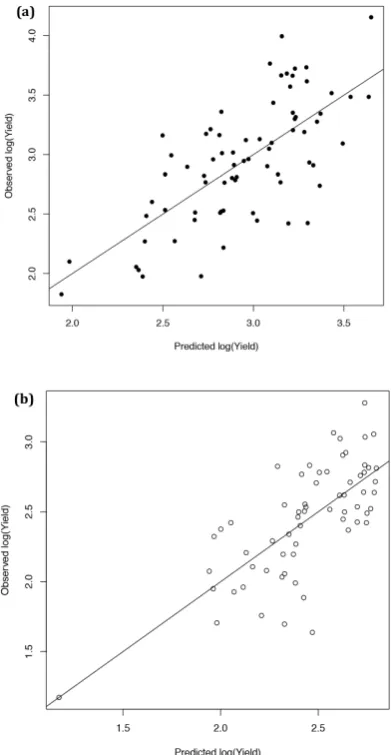
Figure 1. Responses of 35 varieties of Brassica napus to nitrogen fertilizers in Year 1. (a) Comparison 

of observed yield to that predicted by the statistical model for Year 1 data from low (18 kg ha−1_; open 

circle) and high (148 kg ha−1_{; closed circle) nitrogen plots (R}2 _{= 0.5404). (b) Size of the nitrogen effect} 

for each variety. Bars = SEM. Varieties for which the addition of nitrogen had a significant impact on 

yield are marked with *. 

2.2. Genetic Factors Are Stronger Predictors of Yield than Environmental Factors within Year 

Agronomy2017,7, 31 5 of 26

2.2. Genetic Factors Are Stronger Predictors of Yield than Environmental Factors within Year

In order to explore models that could predict yield independently of N application, and in preparation for characterising Year 2 data where only one N treatment was included in the trial, statistical models were developed independently for low and high N treatments (Figure2and Table2). Both models performed slightly less well than the combined model (Figure1a). Each shared some covariates with the combined model, with seeds per pod and seed linolenic acid common between the combined and low N models and log[seed glucosinolate] common between the combined and high N models. There were no common covariates between the low and high N models. Having seed compositional traits as core terms in both the combined and separated models, as opposed to the terms being entirely of growth and development traits, suggests that the combined model is applicable to a range of growing environments. The six terms in the low N model accounted for 52.67% of the variance in yield. The low N treatment demonstrated the importance of senescence when resources are limited; a higher percentage of green pods at the stages examined showed a positive and significant (p< 0.05) relationship with yield (Table2). Variety was excluded as a candidate for this model; however, in a separate model, where only variety was considered, it explained 44.50% of the variation in yield (across all plots), rising to 60.92% in high N plots and 78.43% in low N plots. Therefore, although N does have an impact on yield, the genetic basis of yield (i.e., variety) is a much more powerful predictor.Agronomy 2017, 7, 31    6 of 26 

Figure 2. Comparison of observed yield of 35 varieties of Brassica napus to that predicted by the 

statistical model for Year 1 data using data from (a) high nitrogen (148 kg ha−1_) plots (R2 _{= 0.4922) and} 

(b) low nitrogen (18 kg ha−1_) plots (R2 _= 0.5221).  

2.3. Developing an Improved Model to Explain Yield 

Application of the Year 1 low N model to Year 2 data (the crop was only grown under low N in 

Year 2) showed that the model was poor at explaining yield, being able to only account for 25.48% of 

yield variation (Table 3, Figure 3a). This is half of the yield variation explained by the same model in 

Year 1 (52.67%) and demonstrates that within‐year variation in yield is dominated by genetic factors, 

whilst between‐year variation is strongly influenced by the environmental conditions to which the 

plants were exposed. However, although the estimates of variation for the terms used in the model 

are different between years, we see the same directional effects, i.e., there is a negative estimate of 

variation for seed linolenic acid and a positive estimate of variation for seeds per pod. 

To develop the model further, a second forward selection process was performed to determine 

which traits best explained log[yield] in Year 2. Plants in Year 2 were grown on residual N only, and 

additional traits were recorded. As predicted, variety was highly significant (p = 0.009) in predicting 

log[yield], but as with Year 1, this was not included as a term in the following analyses in order to 

determine  traits  that  contribute  to  the  yield  difference  observed  between  varieties.  Seed 

compositional traits, such as linolenic acid, total seed oil and seed protein content, were important 

Agronomy2017,7, 31 6 of 26

Table 2.Statistical model to explain log[yield] under high and low nitrogen.

High Nitrogen Coefficients Estimate Standard Error t-Value Pr (>|t|) Significance _{Variance Explained}Cumulative %

(Intercept) 1.649 0.833 1.980 0.0518 .

-Seed protein content −0.051 0.018 −2.767 0.0073 ** 33.77

Log[early leaf Mn] 0.632 0.223 2.836 0.0060 ** 40.51

Pod dehiscence Low 0.672 0.282 2.379 0.0202 *

-Pod dehiscence Medium 0.731 0.278 0.268 0.0107 * 46.17

Log[seed glucosinolate] −0.108 0.054 −2.019 0.0475 * 49.26

Low Nitrogen Coefficients

(Intercept) 2.113 0.342 6.180 7.28×10−8 _***

-Seed linolenic acid −0.033 0.021 −1.597 0.1159 - 35.59

Seeds per pod 0.028 0.009 2.995 0.0041 ** 41.66

Pod development: Yellow stage −0.276 0.243 −1.137 0.2602 -

-Pod development: Yellow-green stage −0.048 0.216 −0.222 0.8253 - 52.67 Forty-five traits were considered as candidates for terms in the model. Starting with no terms in the model, terms were added using forward selection (see Methods). Traits that do not appear in the model did not significantly

improve the estimation of log[yield]. The data modelled represented 35 varieties grown at high N (148 kg ha−1_{) and}

low (18 kg ha−1) concentrations in duplicate plots in a randomised block design. Residual standard error: 0.3795 on

67◦of freedom; multipleR-squared: 0.4926; adjustedR-squared: 0.4547; residual standard error: 0.2931 on 57◦of

freedom; multipleR-squared: 0.5267; adjustedR-squared: 0.4769; significance codes: 0.001 ‘***’; 0.01 ‘**’; 0.05 ‘*’;

0.1 ‘.’.

2.3. Developing an Improved Model to Explain Yield

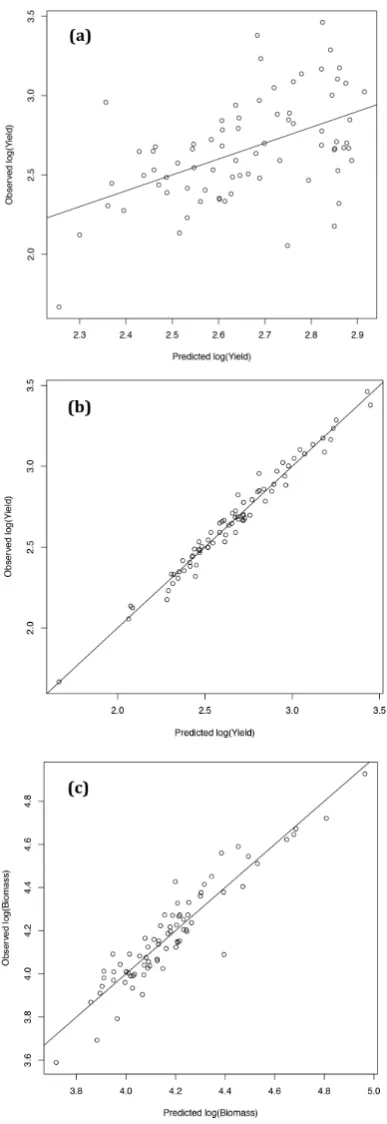
Application of the Year 1 low N model to Year 2 data (the crop was only grown under low N in Year 2) showed that the model was poor at explaining yield, being able to only account for 25.48% of yield variation (Table3, Figure3a). This is half of the yield variation explained by the same model in Year 1 (52.67%) and demonstrates that within-year variation in yield is dominated by genetic factors, whilst between-year variation is strongly influenced by the environmental conditions to which the plants were exposed. However, although the estimates of variation for the terms used in the model are different between years, we see the same directional effects, i.e., there is a negative estimate of variation for seed linolenic acid and a positive estimate of variation for seeds per pod.

To develop the model further, a second forward selection process was performed to determine which traits best explained log[yield] in Year 2. Plants in Year 2 were grown on residual N only, and additional traits were recorded. As predicted, variety was highly significant (p= 0.009) in predicting log[yield], but as with Year 1, this was not included as a term in the following analyses in order to determine traits that contribute to the yield difference observed between varieties. Seed compositional traits, such as linolenic acid, total seed oil and seed protein content, were important factors; however, total vegetative mass (excluding seeds) was the most significant term, explaining 73.70% of log[yield] (Table3, Figure3b). Seed oil was shown to be a positive term, whereas protein content had a negative impact on yield, demonstrating that the oil:protein ratio is important in determining total yield. In total, the forward selection model accounted for 95.12% of the variation contributing to log[yield].

Agronomy2017,7, 31 7 of 26

Agronomy 2017, 7, 31    8 of 26 

Figure 3. Models: (a) Comparing observed yield of Brassica napus in Year 2 to that predicted by the 

statistical model developed on Year 1 data using plants grown on low nitrogen (18 kg ha−1_) plots.   

R2 _{= 0.2548. (b) Explaining yield in Year 2 using forward selection from 133 possible terms. The final} 

model used nine terms to explain 95.12% of the yield variance using plants grown on low nitrogen 

(18 kg ha−1_{) plots in a randomised block design. R}2 _{= 0.951. (c) Explaining vegetative biomass in}   

Year 2 using forward selection from 133 possible terms. The final model used four terms to explain 

80.04% of the biomass variance using plants grown on low nitrogen (18 kg ha−1_{) plots in a randomised} 

block design. R2 _= 0.8004. 

Figure 3.Models: (a) Comparing observed yield ofBrassica napusin Year 2 to that predicted by the statistical model developed on Year 1 data using plants grown on low nitrogen (18 kg ha−1) plots.

Agronomy2017,7, 31 8 of 26

Table 3. Statistical model to explain log[yield] using the Year 1 model on Year 2 data, the forward selection statistical model on Year 2 data and the forward selection statistical model to explain the log[biomass] term from Year 2 data.

Year 1 Model On Year 2 Data

Coefficients Estimate Standard Error t-Value Pr (>|t|) Significance Cumulative % Variance Explained

(Intercept) 2.186 0.325 6.730 3.65×10−9 ***

-Linolenic acid −0.008 0.023 −0.357 0.7224 -

-Seeds per pod 0.012 0.007 1.777 0.0798 .

-Pod development: Yellow stage 0.192 0.103 1.863 0.0666 .

-Pod development: Yellow-green stage 0.332 0.103 3.219 0.0019 **

-Year 2 Model on -Year 2 Data

(Intercept) −2.844 0.494 −5.757 2.42×10−7 _***

-Log[Vegmass] 1.262 0.042 30.377 <2×10−16 *** 73.70%

Total Protein −0.019 0.010 −1.952 0.0551 . 89.16%

Canopy leaf Chlorophyll b 0.337 0.072 4.666 1.55×10−5 _{*** 91.41%}

Total Lipid 0.015 0.006 2.736 0.0204 * 92.04%

Seed weight per pod 0.001 0.000 4.036 0.0001 *** 92.80%

No. pods on primary raceme 0.007 0.001 4.427 3.67×10−5 _{*** 93.50%} Canopy leaf calcium −0.125 0.029 −4.336 5.07×10−5 _{*** 94.40%}

Linolenic acid −0.021 0.008 −2.517 0.0143 * 94.81%

log(Pod Chlorophyll a content Wk43) −0.024 0.012 −2.046 0.0448 * 95.12%

Log[Vegmass] Model on Year 2 Data

(Intercept) 2.423 0.108 22.435 <2×10−16 _***

-Stem area 0.001 0.000 3.407 0.0011 ** 47.16%

Log[No. branches on primary stem] 0.029 0.003 9.574 2.06×10−14 _{*** 59.93%}

Height 0.005 0.001 7.373 2.42×10−10 _{*** 77.74%}

Total branch No. 0.034 0.004 9.793 2.04×10−14 _{*** 75.63%}

Pod carotenoid content (Wk41) 0.021 0.007 2.857 0.005 ** 80.04%

The data modelled represented 35 varieties grown at residual N (~18 kg ha−1_{) in duplicate plots in a randomised}

block design. Residual standard error: 0.2893 on 71◦of freedom; multipleR-squared: 0.2548; adjustedR-squared:

0.2128; residual standard error: 0.07675 on 66◦of freedom; multipleR-squared: 0.9512; adjustedR-squared: 0.9446;

residual standard error: 0.102 on 71◦of freedom; multipleR-squared: 0.8004; adjustedR-squared: 0.7891; significance

codes: 0.001 ‘***’; 0.01 ‘**’; 0.05 ‘*’; 0.1 ‘.’.

2.4. Ten-Fold Cross-Validation of the Year 2 Models

In order to investigate how robust these models are to new data, we divided the plots from Year 2 at random into ten groups (folds). We then fitted the models (estimated the parameters) using nine of the folds and then applied the model to the remaining fold and measured the percentage of variance explained. We repeated this procedure for each of the ten folds in turn. Over the 10 folds, the percentage of variance explained by the yield model ranged from 83.28%–97.90%, with an average of 93.61%. The same approach was applied to the “Vegmass” model, where the average percentage of variance explained was 67.57%. As expected, there is a slight drop in the percentage of variation explained compared to the original model that used all of the available data, but the decrease is not substantial, suggesting that the models are robust to new data obtained from plants grown under similar environmental conditions.

2.5. Seed Oil Content Rather Than Protein Drives Seed Yield

Agronomy2017,7, 31 9 of 26

during development does not necessarily imply that resources will be translocated into seeds at a later stage. Flowering window has a non-significant relationship with yield and biomass. The relationship between the majority of the leaf minerals analysed and yield was also non-significant, the exceptions being canopy leaf potassium, which was strongly negatively correlated with yield (−0.432), total biomass (−0.403) and vegetative biomass (−0.375) and early leaf phosphorus, which was positively correlated with yield (0.281), total biomass (0.384) and vegetative biomass (0.408).

Agronomy 2017, 7, 31    9 of 26 

2.4.

Ten

‐

Fold

Cross

‐

Validation

of

the

Year

2

Models

In

order

to

investigate

how

robust

these

models

are

to

new

data,

we

divided

the

plots

from

Year

2

at

random

into

ten

groups

(folds).

We

then

fitted

the

models

(estimated

the

parameters)

using

nine

of

the

folds

and

then

applied

the

model

to

the

remaining

fold

and

measured

the

percentage

of

variance

explained.

We

repeated

this

procedure

for

each

of

the

ten

folds

in

turn.

Over

the

10

folds,

the

percentage

of

variance

explained

by

the

yield

model

ranged

from

83.28%–97.90%,

with

an

average

of

93.61%.

The

same

approach

was

applied

to

the

“Vegmass”

model,

where

the

average

percentage

of

variance

explained

was

67.57%.

As

expected,

there

is

a

slight

drop

in

the

percentage

of

variation

explained

compared

to

the

original

model

that

used

all

of

the

available

data,

but

the

decrease

is

not

substantial,

suggesting

that

the

models

are

robust

to

new

data

obtained

from

plants

grown

under

similar

environmental

conditions.

2.5.

Seed

Oil

Content

Rather

Than

Protein

Drives

Seed

Yield

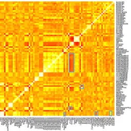
A

correlation

matrix

was

used

to

visualise

positive

and

negative

relationships

between

different

traits

(Figure

4).

The

matrix

showed

(factors

mentioned

in

the

text

below

are

boxed

in

blue

in

Figure

4)

that

the

oil:protein

ratio

was

correlated

positively

with

seed

number

per

pod

(0.756)

and

negatively

with

seed

packing

density

per

pod

(

−

0.702).

This

appeared

to

be

driven

by

the

lipid

component,

since

there

was

a

negative

relationship

between

protein

content

and

seed

weight

per

pod

(

−

0.627).

This

suggests

that

seed

yield

gain

for

an

individual

plant

was

driven

by

increased

oil

content.

There

was

also

a

strong

negative

relationship

between

pigment

(chlorophyll

and

carotenoid)

content

of

the

pod

and

protein/sugars

(range

from

 −

0.239—

−

0.579).

This

implies

that

senescence

may

drive

the

remobilisation

of

sugars

and

proteins

into

the

developing

seed

and

that

retention

of

pigment

in

the

pod

during

development

does

not

necessarily

imply

that

resources

will

be

translocated

into

seeds

at

a

later

stage.

Flowering

window

has

a

non

‐

significant

relationship

with

yield

and

biomass.

The

relationship

between

the

majority

of

the

leaf

minerals

analysed

and

yield

was

also

non

‐

significant,

the

exceptions

being

canopy

leaf

potassium,

which

was

strongly

negatively

correlated

with

yield

(

−

0.432),

total

biomass

(

−

0.403)

and

vegetative

biomass

(

−

0.375)

and

early

leaf

phosphorus,

which

was

positively

correlated

with

yield

(0.281),

total

biomass

(0.384)

and

vegetative

biomass

(0.408).

Figure  4.  Correlation  matrix  showing  the  relationship  between  all  traits  measured  from   

Brassica napus plants in Year 2. White squares = positive correlation of +1; red squares indicate a strong 

negative correlation. Note that where a measurement was taken on multiple occasions, some time 

points are not shown for clarity. Blue squares indicate regions of the matrix that are discussed in the 

main text. 

Figure 4.Correlation matrix showing the relationship between all traits measured fromBrassica napus

plants in Year 2. White squares = positive correlation of +1; red squares indicate a strong negative correlation. Note that where a measurement was taken on multiple occasions, some time points are not shown for clarity. Blue squares indicate regions of the matrix that are discussed in the main text.

Agronomy2017,7, 31 10 of 26

Agronomy 2017, 7, 31    10 of 26 

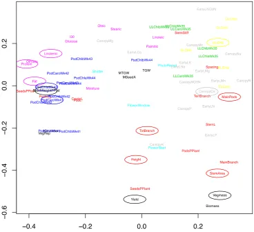
Multi‐Dimensional Scaling (MDS) was used to project the distances between traits in a schematic 

diagram (Figure 5). The correlation between each pair of traits was converted into a distance, where 

a correlation of ±1 was given a distance of zero and a correlation of zero was given a distance of one. 

We then used MDS to show the best two‐dimensional projection of these distances; traits that are 

positioned close together are highly correlated. Traits that the models (Table 3) deem useful for 

predicting yield and/or biomass are circled, and colour is used to group traits according to their type: 

yield, architecture, leaf chlorophyll, pod chlorophyll, progression of plant development, oil/protein 

content and minerals. Biomass, the most important predictor of yield, was located relatively close to 

the yield term, and biomass itself is positioned closely to the architectural traits nearby. The next two 

predictors from the linear yield model, seed protein and canopy leaf chlorophyll b content, are located 

further away from the yield term. Leaf mineral analysis makes no contribution to the yield models. 

Perhaps surprisingly, traits relating to floral development are not important for the yield model, so 

the date of first flower opening, photoperiod, flowering duration and time to pod shatter had no 

significant impact on yield.  

Figure 5. Multi‐dimensional scaling of all traits measured from Brassica napus. The correlation 

between each pair of traits was converted into a distance, where a correlation of ±1 was given a 

distance of zero and a correlation of zero was given a distance of one; a two‐dimensional projection 

of these distances is shown in the figure. Traits that are close together in this space are highly 

correlated. Traits are coloured according to the type of trait: measures of yield (black), architecture 

(red), lower leaf and upper leaf chlorophyll (green), pod chlorophyll (blue), timing of plant 

development (cyan), NIRS data (pink), early leaf and canopy leaf chlorophyll (yellow) and early leaf 

and canopy leaf minerals (grey). Traits used in the models for predicting yield and/or vegetative 

biomass are circled. 

Figure 5.Multi-dimensional scaling of all traits measured fromBrassica napus. The correlation between each pair of traits was converted into a distance, where a correlation of±1 was given a distance of zero and a correlation of zero was given a distance of one; a two-dimensional projection of these distances is shown in the figure. Traits that are close together in this space are highly correlated. Traits are coloured according to the type of trait: measures of yield (black), architecture (red), lower leaf and upper leaf chlorophyll (green), pod chlorophyll (blue), timing of plant development (cyan), NIRS data (pink), early leaf and canopy leaf chlorophyll (yellow) and early leaf and canopy leaf minerals (grey). Traits used in the models for predicting yield and/or vegetative biomass are circled.

Agronomy2017,7, 31 11 of 26

and plant height were positively correlated with yield, together with lipid content and pod weight for all varieties, except Darmor, Rameses and Canard.

Agronomy 2017, 7, 31    11 of 26 

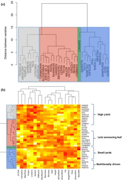
2.6. Analysis of Varieties to Determine Those Produce High Yields and Highlight Gaps in Breeding Potential 

Having established  which  traits  are  important  for predicting  yield (Table 3),  next  we 

investigated which varieties displayed the traits contributing to high yield. For this analysis, we used 

the mean of both blocks for each variety for each trait contributing to the models for yield and above‐

ground  vegetative  biomass  at  harvest  (Table  3).  Each  of  the  traits  was  scaled  to have  a   

mean = 0 and variance = 1. For the cluster analysis, we took the Euclidean distance between each pair 

of varieties and combined varieties using Ward’s method, creating three groups from the whole 

dataset (Figure 6). A combined approach was then taken to include the other traits shown to be 

important in our earlier models and to cluster them all against the varieties studied (Figure 6b). 

Varieties are ordered according to the cluster analysis shown in Figure 6a. The top cluster contains 

all of the highest yielding varieties and the bottom cluster all the lowest yielding varieties. High seed 

protein, seed linolenic acid content, chlorophyll b content of the canopy leaf and early leaf calcium 

content were all negatively correlated with yield; however, it should be noted that canopy leaf 

chlorophyll b was a positive term within the statistical model for log[yield]. This is because the 

correlation is relatively weak with yield (0.11), biomass (0.03) and protein (0.09), so canopy leaf 

chlorophyll b only becomes an important term once biomass and protein are taken into account. 

Conversely, the architectural plant traits of raceme area and plant height were positively correlated 

with yield, together with lipid content and pod weight for all varieties, except Darmor, Rameses   

and Canard.  

Figure 6. Cluster analysis of the Brassica napus traits and varieties. (a) Cluster dendrogram of the 

variety set; each cluster is blocked in green, black (grey), red or blue to correspond with Figure 6b and 

the colours used to circle varieties in Figure 7. The study included 35 different plant varieties. The 

mean of both blocks was used for each variety for each trait; each of the traits was scaled to have a 

mean = 0 and variance = 1, and then cluster analysis was performed by taking the Euclidean distance 

between each pair of varieties and combining varieties using Ward’s method. The distance between 

varieties is defined as equal to the sum of the squares of differences across all traits analysed in Figure 

5. (b) Analysis of the traits contributing to the yield and vegetative biomass models clustered by 

variety. 

Figure 6. Cluster analysis of theBrassica napustraits and varieties. (a) Cluster dendrogram of the variety set; each cluster is blocked in green, black (grey), red or blue to correspond with Figure6b and the colours used to circle varieties in Figure7. The study included 35 different plant varieties. The mean of both blocks was used for each variety for each trait; each of the traits was scaled to have a mean = 0 and variance = 1, and then cluster analysis was performed by taking the Euclidean distance between each pair of varieties and combining varieties using Ward’s method. The distance between varieties is defined as equal to the sum of the squares of differences across all traits analysed in Figure5. (b) Analysis of the traits contributing to the yield and vegetative biomass models clustered by variety.

Agronomy2017,7, 31 12 of 26

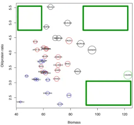
Agronomy 2017, 7, 31    12 of 26 

In the model for explaining yield, the top two terms were vegetative biomass (positive) and total 

protein (negative). Total seed oil also (positively) contributed to yield. Therefore, the oil:protein ratio 

and biomass traits were used to illustrate the clustering of different varieties in two‐dimensional 

space (Figure 7). Canard produced the highest yield, but had a comparatively low oil:protein ratio. It 

also had a very poor score for raceme stiffness and has been observed to lodge readily in the field; 

therefore, although Canard had a high vegetative biomass, the architecture was not sufficiently 

robust. The varieties from the cluster coloured grey also had high yield, but show a higher oil:protein 

ratio than other clusters, meaning that the yield increase is achieved by assimilating more oil in the 

seeds. The other groups had lower vegetative biomass, lower oil:protein ratio and lower yield, with 

Ningyou having the poorest phenotype of all of the varieties. Yield gaps are apparent (green squares 

on Figure 7) where breeding and selection, or agronomy, could be used to target plants with high oil 

content from a smaller vegetative biomass (by changing the harvest index to put more resources into 

seeds), or large plants with high yields of oil‐rich seeds, or large plants with low oil content that could 

potentially be used as biomass crops.  

Figure 7. Varietal distribution across the Brassica napus diversity trial in two‐dimensional space using 

vegetative biomass and oil:protein ratio. The yield of each variety is shown by the radius of the circle; 

colours are used to identify the varieties within each cluster as determined in Figure 6. Green boxes 

indicate yield gaps where no varieties currently exist. 

2.7. Traits Measured Early in Crop Development Are Also Good Predictors of Yield 

Our earlier model for explaining yield (Table 3) relied on many traits that can only be observed 

at, or close to, the time of harvest. While that model is useful for selecting the variety for growing in 

subsequent seasons, a model that forecasts yield during the growing period would also be more 

useful. Traditional early observations, such as date of flowering and leaf chlorophyll retention, had 

very poor correlation with seed yield (Figure 8). 

Observations in the field of the highest and lowest yielding varieties showed that there was very 

little visual difference in colour of pods on the main raceme from May–July (Figure 9a), although the 

absolute leaf chlorophyll levels in April demonstrated clear differences between the varieties (Figure 

8). However, when the canopy was viewed as an entirety, there were clear differences in senescence 

Figure 7.Varietal distribution across theBrassica napusdiversity trial in two-dimensional space using vegetative biomass and oil:protein ratio. The yield of each variety is shown by the radius of the circle; colours are used to identify the varieties within each cluster as determined in Figure6. Green boxes indicate yield gaps where no varieties currently exist.

2.7. Traits Measured Early in Crop Development Are Also Good Predictors of Yield

Our earlier model for explaining yield (Table3) relied on many traits that can only be observed at, or close to, the time of harvest. While that model is useful for selecting the variety for growing in subsequent seasons, a model that forecasts yield during the growing period would also be more useful. Traditional early observations, such as date of flowering and leaf chlorophyll retention, had very poor correlation with seed yield (Figure8).

Agronomy 2017, 7, 31    13 of 26 

between the high and low yielding varieties (Figure 9b) with high yielding plants having a slower 

senescing canopy. When the extreme lines (defined as the top ten lines for seed yield, retention of 

pod chlorophyll and biomass) were analysed, only two high yielding cultivars, Canard and Victor, 

also had high biomass and slow pod senescence. In other cases, high biomass lines overlapped with 

high yielding lines, but retention of pod chlorophyll did not correlate well (Figure 10a).   

Figure 8. Scores for nine traits associated with resource allocation and yield for the thirty‐five varieties 

used in this study, ordered by yield (outer ring) and coloured from largest (red) to smallest (green) in 

each  ring.  Averages  of  all  replicates  over  both  blocks  were  used.  White   

spaces = missing data. 

It was essential to develop a model that can predict final yield prior to visual indicators of yield 

differences. The forward selection procedure was repeated, but only allowing covariates that were 

unrelated to flowers or pods in the model. The fitted model (Table 4, Figure 10b) explains 63.69% of 

the variance in yield, compared to 95.12% in the earlier model (Table 3). This reduction was due to 

the omission of information regarding the later stages of plant development. However, the model 

still offers a good method for predicting yield approximately 15 weeks prior to harvest, i.e., 

approximately April of the same year. The model comprises two of the best architectural variables 

(stem area and numbers of branches on the primary stem) that were used to explain vegetative 

biomass in the earlier model. Canopy leaf chlorophyll b content, which was in the earlier model for 

predicting yield, was also included in the predictive model (Table 4). Interestingly, two leaf mineral 

concentration traits were also selected, canopy leaf potassium and canopy leaf magnesium.  

Agronomy2017,7, 31 13 of 26

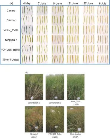
Observations in the field of the highest and lowest yielding varieties showed that there was very little visual difference in colour of pods on the main raceme from May–July (Figure9a), although the absolute leaf chlorophyll levels in April demonstrated clear differences between the varieties (Figure8). However, when the canopy was viewed as an entirety, there were clear differences in senescence between the high and low yielding varieties (Figure9b) with high yielding plants having a slower senescing canopy. When the extreme lines (defined as the top ten lines for seed yield, retention of pod chlorophyll and biomass) were analysed, only two high yielding cultivars, Canard and Victor, also had high biomass and slow pod senescence. In other cases, high biomass lines overlapped with high yielding lines, but retention of pod chlorophyll did not correlate well (Figure10a).

Agronomy 2017, 7, 31    14 of 26 

Figure 9. Contrast in uniformity of Brassica napus. (a) Pod senescence on primary stems and   

(b) Canopy senescence. Canard, Darmor and Victor TVSL are the three highest yielding lines; 

Ningyou7, POH285 and Shen‐li Jutsai are the three lowest yielding in terms of seed mass per plant. 

Dates in (a) are the dates the images were taken. All images in (b) were taken on 13 June 2011, with 

the dates shown in brackets being the final harvest date for each line.  

Table 4. Forward selection statistical model to predict the yield from traits observable at or prior to 

flowering using Year 2 data. The data modelled represented 35 varieties grown at residual N   

(~18 kg ha−1_{) in duplicate plots in a randomised block design.}  

Coefficients  Estimate  Standard 

Error  t‐Value  Pr(>|t|)  Significance 

Cumulative % Variance 

Explained 

(Intercept)  −0.377  0.359  1.050  0.2975  ‐  ‐ 

Agronomy2017,7, 31 14 of 26

Agronomy 2017, 7, 31    15 of 26 

Stem area  0.002  0.001  3.150   0.00241  **  36.64% 

Log[No. branches on 

primary stem]   0.724  0.151  4.811  8.51 x 10‐6  ***  44.22% 

Length of flower set  0.009  0.003  3.294  0.0016  **  51.73% 

Canopy leaf potassium  −0.188  0.057  −3.293  0.0016  **  56.92% 

Canopy leaf chlorophyll b  0.550  0.185  2.972  0.0041  **  60.19% 

Canopy leaf Mg  1.594  0.617  2.582  0.0120  *  63.69% 

Residual standard error: 0.2048 on 69° of freedom; multiple R‐squared: 0.6369; adjusted R‐squared: 

0.6054; significance codes: 0.001 ‘***’; 0.01 ‘**’; 0.05 ‘*’. 

Figure 10. Plant traits as drivers for final yield in Brassica napus. (a) Top 10 lines in each category 

showing overlap between them. Temple is one of the most commonly‐grown varieties, yet it is 

atypical in linking chlorophyll retention to high yield. In general, biomass and yield overlap (big 

plants = more seed) and varieties with a delayed senescence phenotype do not yield highly.   

(b) Model for predicting yield using traits that were observed at or before the time of flowering. The 

model was developed using nine terms and applied to Year 2 data collected from plants grown on 

low nitrogen (22 kg ha−1_{) plots in a randomised block design. R}2 _= 0.6369. 

3. Discussion 

Seed yield is a complex trait influenced by numerous interacting variables that are governed by 

both genetic and environmental factors. Several studies have sought to understand the contribution 

of individual traits to oilseed rape yield [4,6,32–35] or to model yield such that it can be predicted 

over future growing seasons [5,7,8,36]. However, there is some disagreement between the studies as  Figure 10. Plant traits as drivers for final yield inBrassica napus. (a) Top 10 lines in each category showing overlap between them. Temple is one of the most commonly-grown varieties, yet it is atypical in linking chlorophyll retention to high yield. In general, biomass and yield overlap (big plants = more seed) and varieties with a delayed senescence phenotype do not yield highly. (b) Model for predicting yield using traits that were observed at or before the time of flowering. The model was developed using nine terms and applied to Year 2 data collected from plants grown on low nitrogen (22 kg ha−1₎

plots in a randomised block design.R2= 0.6369.

Agronomy2017,7, 31 15 of 26

Table 4. Forward selection statistical model to predict the yield from traits observable at or prior to flowering using Year 2 data. The data modelled represented 35 varieties grown at residual N (~18 kg ha−1) in duplicate plots in a randomised block design.

Coefficients Estimate Standard Error t-Value Pr (>|t|) Significance Cumulative % Variance Explained

(Intercept) −0.377 0.359 1.050 0.2975 -

-Stem area 0.002 0.001 3.150 0.00241 ** 36.64%

Log[No. branches on primary stem] 0.724 0.151 4.811 8.51×10−6 _{*** 44.22%}

Length of flower set 0.009 0.003 3.294 0.0016 ** 51.73%

Canopy leaf potassium −0.188 0.057 −3.293 0.0016 ** 56.92%

Canopy leaf chlorophyll b 0.550 0.185 2.972 0.0041 ** 60.19%

Canopy leaf Mg 1.594 0.617 2.582 0.0120 * 63.69%

Residual standard error: 0.2048 on 69◦of freedom; multipleR-squared: 0.6369; adjustedR-squared: 0.6054;

significance codes: 0.001 ‘***’; 0.01 ‘**’; 0.05 ‘*’.

3. Discussion

Seed yield is a complex trait influenced by numerous interacting variables that are governed by both genetic and environmental factors. Several studies have sought to understand the contribution of individual traits to oilseed rape yield [4,6,32–35] or to model yield such that it can be predicted over future growing seasons [5,7,8,36]. However, there is some disagreement between the studies as to what are the most important traits that influence yield, be it the number of pods per plant [34], the time to maturity [6] or the duration of flowering [32]. One of the reasons for the discrepancies observed between the different studies is the limitations in the number or type of traits that were measured or the use of a limited number of cultivars, which constrained the genotypic variation that could be observed.

3.1. Greater Branching Density Drives Yield Improvement

Oilseed rape architectural traits accounted for the greatest percentage of variation in above-ground biomass at harvest. Significant positive correlations were observed between both total above-ground biomass and vegetative biomass and seed yield. Thus, although partitioning more resources into vegetative development could be seen to divert resources away from reproductive development, a larger above-ground biomass with increased branching, supported by a larger stem and taller plants, gives rise to more available positions upon which pods can develop. In this study all plots were planted at the same seed rate within year, but it is well established that lower seed rates can be used to produce plants with more branches than those in tightly-packed canopies [37].

Agronomy2017,7, 31 16 of 26

pod, leaf or flower can be regarded as indispensable [43], and it is known that oilseed rape produces more flowers than are required to obtain maximum yield [35].

3.2. Increasing Seed Oil:Protein Ratio

The model also showed that seed oil and protein were important drivers of yield; indeed, the oil:protein ratio (derived from the seed protein and oil terms used in Model 3b) explains a further 8.1% of the variation within yield, once biomass is taken into account. Grami et al. [44] also established that seed oil content is negatively correlated with protein content; therefore, increasing the oil fraction of the seed would naturally enhance the oil:protein ratio and, according to our model, potentially help increase yields independently of changing architectural traits, although the mechanism by which this conversion occurs is presently not clear. A recent study usingArabidopsispopulations established that seed carbon and N content were antagonistic and that % N was negatively correlated with yield [45], as it is in the present study. InArabidopsis, the number of seeds and pods per plant were closely related to the concentration of seed oil and protein within the seeds [19]. It was shown for soybean that a 1-kg−1increase in oil content will usually lead to a 2-kg−1decrease in protein due to a negative genetic correlation between the two yield components [46]; therefore, changing the oil:protein ratio towards oil production would naturally influence seed yield when defined as the total weight of seeds per plant. None of the lines studied have both a high above-ground biomass and a high oil:protein ratio, a combination that would be predicted to produce even greater yields than those recorded. The lines that show the greatest above-ground biomass (and highest seed yields) could also have their vegetative material utilised for the production of bioethanol and biogas, easing competition with food crops for land and resources. Whilst this technology is still being developed, especially in the case of appropriate pre-treatments to extract sugars from the lignocellulosic plant cell walls, yields of 20.4 g methane 100 g−1_{DM and 10.9 g ethanol 100 g}−1_{DM have been reported for oilseed rape [47].} Although these values are much lower than those for sugarcane (37 g ethanol 100 g−1DM) [48], it is still a useful by-product of oilseed rape production and a technology under development.

In the current study, there was only limited variation between the lines in terms of seed total oil content (45%–58%), but the range of individual fatty acids was highly variable between varieties (Table S1). Many of the oilseed rape varieties grown commercially are High Oleic acid, Low Linolenic acid (HOLL) and the current population contained HOLL and non-HOLL varieties. Seed linolenic acid was consistently and negatively associated with yield; a reflection of the breeding programme that has already taken place to increase yield simultaneously with developing varieties that produce healthy, low trans-fat and stable frying oils and have good disease resistance [49]. It also demonstrates that our model is robust and a true reflection of the genetic basis of yield. Transgenic or mutation (TILLING) technologies would appear to be the most effective method of manipulating the composition of fatty acids within the seed such that it fits the purpose of use, be it for the production of lubricants in industry, or of edible vegetable oils [50], or as a way of producing omega 3-rich oils to enter the human food chain [51]. For example, expressing the yeast gene glycerol-3-phosphate dehydrogenase (gpd1) under the control of a seed-specific promoter increasedB. napusseed oil content by 40% [52].

3.3. Early Leaf P Status Correlates with Final Yield

Agronomy2017,7, 31 17 of 26

to develop, it could provide a useful early indicator of seed yield. Equally, raceme width at the time of flowering was a good indicator of biomass and capable of predicting 36.64% of yield. Similarly, a study in maize found that measurements of raceme width early in the growing season also provided a good predictor of final yield [57]; these early indicators of yield could be used by growers to modify inputs and optimise yield in order to maximise profit margins.

3.4. Number of Pods Determines Yield

The model presented here used the weight of seeds per plant as a measure of yield; however, we also explored whether other parameters of yield, which are used commercially, such as TGW or the number of seeds per pod, could be used as a measure of final seed yield. From the correlation matrix, it became evident that traits previously used as a proxy for seed yield per plant, such as the number of seeds per pod [58], seed weight per pod [59], pod length [60] and even TGW, were not significantly correlated with seed yield per plant in this study (Figure4). This finding indicates that current commercially-used measures, such as TGW, may not be the most appropriate indicator of yield for breeding and selection purposes. Only the numbers of seeds per plant and pods per plant were significantly correlated with seed yield per plant. This indicates that the pod in B. napusis a fairly conserved organ and that a plant will preferentially invest in the production of more pods per plant as opposed to increasing the number or mass of seeds within an individual pod. Once a seed contains the minimum amount of resources necessary to ensure germination viability, then there is no advantage for a plant in investing more resources beyond this in an individual seed, and a better survival strategy is to make more seeds in different pods, a view also reported in a study onArabidopsis resource allocation [19]. Similarly, the addition of N was found to increase oilseed rape yields through the production of more pods as opposed to affecting individual seed or pod weight [33], something also observed in Year 1 of the current trial where plants were grown on high and low N.

3.5. Flowering Start Date and Duration Do Not Affect Seed Yield

Oilseed rape has been bred to be self-fertile, but it can also be pollinated by wind and insects; the latter was found to enhance seed oil content quality, potentially due to the ability of insects to optimise the timing of fertilisation for the plant [61]. InArabidopsisgrown under controlled conditions, initially under short days and then switched to long days to induce flowering, the plants that flowered later had a lower yield [17]. In contrast, in the current field-based study, it was found that the flowering start date and flowering window were related neither to the number of pods per plant, nor to seed yield. Thus, increasing the flowering duration does not appear to increase pollination efficiency, perhaps because the general decline in pollinators within agricultural systems [62] means insufficient exploitation of the additional flowers. The increased early flowering nature of lines with long flowering duration may also have increased the unwanted presence of pollen beetle pests (Meligethesspp.), which are attracted by the visual and olfactory properties of oilseed rape flowers [63]. Thus, within the current field trial, the unopened buds on plants of those lines that flowered earlier may have been at increased risk from feeding damage than those on plants not yet flowering, especially if pollen resources were scarce due to high intraspecific competition, and this may partly explain why it did not afford a yield advantage to be flowering earlier or over a longer period.

3.6. The Relationship between Plant Senescence and Seed Yield