Nonlinear signal correction observer and application to UAV navigation

Nonlinear signal-correction observer and

application to UAV navigation

Xinhua Wang, Weicheng Wang

Abstract—A nonlinear signal-correction observer (N-SCO) is presented for signals correction and estimation, which not only can reject the position measurement error, but also the unknown velocity can be estimated, in spite of the existence of large position measurement error and intense stochastic non-Gaussian noise. For this method, the position signal is not required to be bounded. The N-SCO is developed for position/acceleration integration, and it is applied to an unmanned aerial vehicle (UAV) navigation: Based on the NSCO, the position and flying velocity of quadrotor UAV are estimated. An experiment is conducted to demonstrate the effectiveness of the proposed method.

Index Terms—Large position measurement error, nonlin-ear signal-correction observer (NSCO), UAV.

I. INTRODUCTION

P

OSITION and velocity play the key roles for system navigation and control. For position recognition, global positioning system (GPS) is usually adopted and supplemented by some sensors [1,2,3]. On the one hand, GPS can provide the instantaneous large-error position of device, and the posi-tion signal is usually contaminated by the circumstances [2]. Velocity is also necessary for navigation and control, and the velocity of device can be estimated by the optical flow sensors (OFS) [4]. Nevertheless, they are sensible to lighting changes. The state observers [5,6,7] are popular to estimate velocity from position measurement. In [5], a full-order observer was designed for the state estimation of the systems with unknown inputs. However, the above observers are not suitable to the systems with large position measurement errors. On the other hand, an inertial navigation systems (INS) with the integrators [8,9] can provide position and velocity information, but it usually suffers from signal drifts over time. Several observer-based INS methods were used to estimate the position and velocity [10,11,12]. In [11], a dynamic observer was designed to estimate position. However, the position trajectory is required to be bounded in a constraint range, and it is not suitable to large-range navigation.

The integration of GPS and INS can limit the shortcomings of the individual systems [13,14,15], and the integration can improve the accuracy of GPS outputs. The present GPS/INS

Manuscript received January 29, 2018; revised May 07, 2018 and May 31, 2018; accepted July 11, 2018.(Corresponding author: Xinhua Wang.)

Xinhua Wang is with the Department of Electrical and Electronic Engineering, University of Nottingham, Nottingham, NG7 2RD, U.K. (e-mail: [email protected]; [email protected]).

Weicheng Wang is with the Huatimesee UAV Design Company, Beijing, China (e-mail: [email protected]).

integrations are mostly based on Kalman filter (KF): KF for linear systems [16], and extended Kalman filter (EKF) for the first order approximation to nonlinear systems [17]. KF (or EKF) can separate the probabilistic noise and can estimate position and velocity based on the optimization of a recursive least mean square error. However, in GPS/INS integration, the KF and EKF algorithms have several limitations: i) Noise is assumed to be zero-mean Gaussian distributed, and the process noise covariance is uncorrelated to the estimation error. As stochastic non-Gaussian noise exists in signal, the inaccurate noise information may lead to the position and velocity drifts. ii) The accurate priori information of the covariance matrices of the noises is needed. However, the noise levels may change in different applications and circumstances. iii) System linearization may cause filter divergence, and the derivation of the Jacobian matrices are nontrivial.

Considering the problems above, in this paper, a NSCO is designed to integrate the measurement signals, to reject the large position measurement error, and to estimate the unknown velocity. Inspired by the finite-time stability and robustness of autonomous systems [18,19] and singular perturbations [20], the NSCO is developed, which can minimize the position sensor error, and can estimate the unknown velocity in spite of the existence of stochastic non-Gaussian noise. The parameters selection of NSCO is satisfied with the Routh-Hurwitz Sta-bility Criterion. Moreover, the performances of the proposed NSCO are compared with those of the EKF.

the flight dynamics.

II. CONFIGURATION OFNSCO

The goal of the NSCO design is to reject the position measurement error, and to estimate the unknown velocity through the signals integration.

A. Case of position/acceleration integration

We consider the following case of system navigation: 1) GPS provides the large-error position a1(t) =a01(t) +

d1(t), where a01(t) is real position, d1(t) is the large

mea-surement error, and sup_t∈[0,∞)|d1(t)| ≤L1<∞;

2) INS gives the accelerationa3(t) =a03(t) +d3(t), where

a03(t) is real acceleration, d3(t) is the measurement error,

sup_t∈[0,∞)|d3(t)| ≤L3<∞, andL3≪L1;

3) The velocity a02(t) is unknown.

For the real positiona01(t), velocitya02(t)and acceleration

a03(t), the relations a01(t) =

∫t 0

∫υ

0 a03(σ1)dσ1dσ2 and

a02(t) =

∫t

0a03(σ)dσ hold.

Question: How to estimate the real position a01(t) and

the velocity a02(t) of device from the measurements of the

position a1(t) =a01(t) +d1(t)and the acceleration a3(t) =

a03(t) +d3(t), in spite of the existence of the large position

measurement error and stochastic non-Gaussian noise?

B. Definition of NSCO

The usual observers, for instance, sliding mode observers, can estimate the unknown states based on the small-error position measurement a1(t). For the following sliding mode

observer (See Theorem 6 in [28])

˙

x1 = x2−λ1|x1−a1(t)| 2 3_sign(x

1−a1(t))

˙

x2 = x3−λ2|x1−a1(t)| 1 3_sign(x

1−a1(t))

˙

x3 = −λ3sign(x1−a1(t)) (1)

if the sensor error exists in the measurement signala1(t), i.e.,

a1(t) = a01(t) +d1(t), where a01(t) is real position, d1(t)

is the small position measurement error,sup_t∈[0,∞)|d1(t)| ≤

L1 < ∞, then there exist µ > 0 andts >0, such that, for t≥ts,

|xi−a0i(t)| ≤µL 4−i

3

1 , i= 1,2,3 (2)

The observer is suitable to estimate velocity a02(t) and

accelerationa03(t)from the small-error position measurement

a1(t) =a01(t)+d1(t). However, they cannot reject sufficiently

the effect of large position errord1(t): if the large errord1(t)

exists in the measurement signal a1(t) = a01(t) +d1(t),

the up-boundnessL

4−i

3

1 of the estimation errors is also large.

Therefore, the usual observers are not suitable to the systems with large position measurement errors.

Actually, the measurements for the usual navigation systems include the large-error position measurement by GPS and the small-error acceleration measurement by INS. For system navigation, the accurate position and velocity are needed.

Definition 1 (NSCO):For the large-error position measure-menta1(t) =a01(t) +d1(t)and small-error acceleration

mea-surementa3(t) =a03(t)+d3(t), where,d1(t)andd3(t)are the

unknown large and small measurement errors, respectively, a nonlinear signal-correction observer (NSCO) is designed, such that the large position measurement error can be rejected and the unknown velocity is estimated.

The configuration of a NSCO is described by

˙

x1 = x2; x˙2=x3;

˙

x3 = f(x1−a1(t), x2, x3−a3(t)) (3)

with the conclusions:

x1→a01(t), x2→a02(t), x3→a03(t) (4)

In the above NSCO configuration, the system inputs include the position measurementa1(t)and acceleration measurement

a3(t). The states x1, x2 and x3 estimate the real position

a01(t), velocity a02(t) and acceleration a03(t), respectively.

Importantly, the large sensor error d1(t)in position

measure-ment a1(t) will be rejected sufficiently, and the position and

velocity drifts will be avoided even non-Gaussian noise exists.

III. DESIGN OF NSCO

In the following, considering the large position sensor error and stochastic non-Gaussian noise, a NSCO is designed to to reject the position measurement error and to estimate the velocity. The position is not required to be bounded. One theorem is presented as follows.

A. NSCO for position/acceleration integration

Theorem 1:Considering Case A in Section II, for system

˙

x1 = x2; x˙2=x3;

ε4x˙3 = −k1|ε(x1−a1(t))|

α1_sign(x

1−a1(t))

−k2ε2x2 α2

sign(x2)

−k3|(x3−a3(t))|α3sign(x3−a3(t)) (5)

whereε∈(0,1)is the perturbation parameter;

k1>0, k3>0, k2> ε3α3

k1

k3

(6)

andα1, α2, α3 satisfy

α3∈(0,1), α2=

α3

2−α3

, α1=

α3

3−2α3

(7)

1) if the sensor errors exist in the measurement signalsa1(t)

anda3(t), i.e., a1(t) =a01(t) +d1(t)anda3(t) = a03(t) +

d3(t), wherea01(t)is real position,d1(t)is the large position

measurement error, sup_t∈[0,∞)|d1(t)| ≤ L1 < ∞, a03(t) is

real acceleration,d3(t)is the acceleration measurement error,

sup_t∈[0,∞)|d3(t)| ≤L3<∞, andL3≪L1, then there exist

L >0,γ > _α4

1 andΓ>0, such that, for t≥εΓ (Ξ(ε)e(0)),

where, δdi = εα1−

i

γ ₊2

1−α3_k3Lα3 3

δ0 ε

−i

γ ∈ _{(0,1), i = 1,2,3;}

δ0 = 2

∑

i=1

21−αi_k

iLαii +La; supt∈[0,∞)|a˙03(t)| ≤ La < ∞; γ= (1−β)/β,β∈(0, α1/(α1+ 4));Ξ(ε) =diag{ε, ε2, ε3},

andei=xi−a0i(t),i= 1,2,3;e= [ e1 e2 e3 ]T.

2) Furthermore, assume there is no sensor error in signal a3(t), i.e.,a3(t) =a03(t), then, even large sensor error exists

in signala1(t), fort≥εΓ (Ξ(ε)e(0)),

|xi−a0i(t)| ≤Lεα1γ−i, i= 1,2,3 (9) The proof of Theorem 1 is presented in Appendix.

B. Robustness analysis in frequency domain

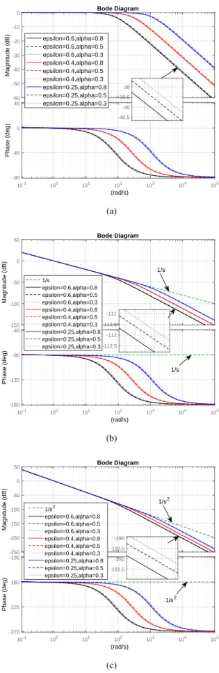
In practice, high-frequency noises exist in measurements a1(t)anda3(t). For the NSCO, frequency-sweep method [29]

can be used to approximately analyse the nonlinear behaviors of the NSCO, and the Bode plots are adopted to describe the system frequency characteristics. By frequency-sweep method, we can find that the NSCO leads to perform precise estimation and strong rejection of high-frequency noise.

The test of frequency characteristic can be implemented by Bode plot fitting. The input signals are selected as: acceleration a3(t) = Amsin(ωt), and position a1(t) = −A_ωm2 sin(ωt),

whereAm andω are the amplitude and angular frequency of the input signala3(t), respectively. The outputs arex3,x2and

x1. Equivalently,a3(t)can be taken as the unique input signal,

and a1(t)is the double integral of a3(t). The Bode plots of

the relations a3(t) → x3, a3(t) → x2 and a3(t)→ x1 will

be sketched, respectively. In fact, for the above input-output relations, the ideal operators are1,1/sand1/s2_{, respectively.}

For the NSCO, the parameters are selected as follows: k1 = 0.5, k2 = 0.2, k3 = 10; α3 = α = 0.8,0.5,0.3;

ε= 0.6,0.4,0.25, respectively. The Bode plots with different selections of ε and α3 are described in Fig.1:

Figs.1(a)-(c) present the frequency characteristics of the acceleration, velocity and position estimations, respectively.

Comparing with ideal operators1/sand1/s2_{, not only the}

NSCO can obtain their estimations of velocity and position precisely, but also the high-frequency noise is rejected suffi-ciently: asω→ ∞, the magnitude tends −∞.

Parameter εaffects the low-pass frequency bandwidth: De-creasing the perturbation parameterε, the low-pass frequency bandwidth becomes larger, and the estimation speed becomes fast; on the other hand, increasing perturbation parameter ε, the low-pass frequency bandwidth becomes smaller, and much noise can be rejected sufficiently (See the cases of ε = 0.6, ε = 0.4 and ε = 0.25 in Figs.1 (a)-(c), respectively). Parameter α3 ∈ (0,1) affects the decay speed of frequency

characteristic curves near the cut-off frequency (See the cases of α3 = α = 0.8,0.5,0.3 in Fig.1, respectively): smaller

α3∈(0,1)can obtain more precise estimations; on the other

hand, larger α3 ∈ (0,1) can reduce much noise, however, a

bit estimation delay happens.

Remark 1 (Analysis of NSCO):

1) Stability and robustness of NSCO: In NSCO (5), xi estimates the desired valuesa0i(t),i= 1,2,3, respectively. In

-60 -50 -40 -30 -20 -10 0

Magnitude (dB)

10-1 ₁₀0 ₁₀1 ₁₀2 ₁₀3 ₁₀4 ₁₀5

-90 -45 0 45

Phase (deg)

epsilon=0.6,alpha=0.8 epsilon=0.6,alpha=0.5 epsilon=0.6,alpha=0.3 epsilon=0.4,alpha=0.8 epsilon=0.4,alpha=0.5 epsilon=0.4,alpha=0.3 epsilon=0.25,alpha=0.8 epsilon=0.25,alpha=0.5 epsilon=0.25,alpha=0.3

Bode Diagram

(rad/s)

-40.5 -40 -39.5 -39

(a)

-150 -100 -50 0 50

Magnitude (dB)

10-1 100 101 102 103 104 105

-180 -135 -90 -45

Phase (deg)

1/s

epsilon=0.6,alpha=0.8 epsilon=0.6,alpha=0.5 epsilon=0.6,alpha=0.3 epsilon=0.4,alpha=0.8 epsilon=0.4,alpha=0.5 epsilon=0.4,alpha=0.3 epsilon=0.25,alpha=0.8 epsilon=0.25,alpha=0.5 epsilon=0.25,alpha=0.3

Bode Diagram

(rad/s)

-112.5 -112 -111.5 -111

1/s

1/s

(b)

-250 -200 -150 -100 -50 0 50

Magnitude (dB)

10-1 ₁₀0 ₁₀1 ₁₀2 ₁₀3 ₁₀4 ₁₀5

-270 -225 -180 -135

Phase (deg)

1/s2

epsilon=0.6,alpha=0.8 epsilon=0.6,alpha=0.5 epsilon=0.6,alpha=0.3 epsilon=0.4,alpha=0.8 epsilon=0.4,alpha=0.5 epsilon=0.4,alpha=0.3 epsilon=0.25,alpha=0.8 epsilon=0.25,alpha=0.5 epsilon=0.25,alpha=0.3

Bode Diagram

(rad/s)

-191.5 -191 -190.5 -190

1/s2 1/s2

(c)

the estimation error (9), due toε∈(0,1)andα1γ−i≫1, the

up-boundness of estimation errorLεα1γ−i _{(where,i= 1,2,3)}

is sufficiently small. Therefore, the NSCO leads to perform strong rejection of persistent sensor errors and disturbances, and high-precision signal estimations are achieved. Further-more, from the frequency-domain analysis (See Fig. 1), the NSCO can reject the high-frequency noise.

2) Large position error rejection and velocity estimation:In the NSCO (5), the position is not required to be bounded. The large sensor errord1(t)(where,supt∈[0,∞)|d1(t)| ≤L1<∞)

in the position measurement a1(t) = a01(t) +d1(t) can be

rejected sufficiently. In fact, based on the singular perturbation technique and nonlinear contraction mapping theory, from (30) in the proof of Theorem 1, the effect of the sensor error d1(t)is compressed into21−α1k1Lα11ε

α1_{. Furthermore, in the}

estimation error (9), due to ε ∈ (0,1), the up-boundness of the position estimate error Lεα1γ−1 _{is sufficiently small, and}

Lεα1γ−1≪_L

1. Therefore, the measurement error in position

signal can be rejected sufficiently.

In the estimate error (9), due toε∈(0,1), the up-boundness of the velocity estimate error Lεα1γ−2 _{is small enough.}

3) No drift phenomenon:From (8), in spite of the existence of the large sensor error and non-Gaussian noise, the estimate errors are bounded, and their up-boundnesses are unrelated to time after t≥εΓ (Ξ(ε)e(0)). Therefore, even for unbounded position navigation, no drift phenomenon happens.

Remark 2 (The rules of NSCO parameters selection): For the NSCO, there are several rules on the parameters selection:

1) Basic stability condition:The parameters (k1, k2, k3) and

(α1, α2, α3) are satisfied with Eqs. (6) and (7), respectively.

2) For rejecting the measurement error in position: When the measurement errord1(t)in position signala1(t)increases,

i.e.,L1increases, in order to decrease the error effectk1Lα11 of

δ0= 2

∑

i=1

21−αi_k

iLαii+Lain (30), parameterk1>0decreases

to improve the estimate precisions. Furthermore, in order to decrease Lα1

1 , α1 ∈ (0,1) should decrease to improve the

estimate precisions.

3) For low-pass filtering:In order to increase the estimation speed, ε ∈ (0,1) should decrease to make the low-pass frequency bandwidth larger, orα3∈(0,1)decreases. If much

noise exists,εshould increase, orα3∈(0,1)increases. Thus,

the low-pass frequency bandwidth becomes smaller, and the noise can be rejected sufficiently (See Fig. 1).

IV. UAVNAVIGATION BASED ONNSCO

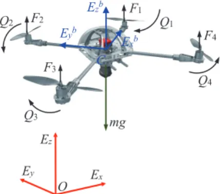
A quadrotor UAV navigation is studied. In this scenario, the large-error position measurement of UAV is considered. The forces and torques of quadrotor UAV are described in Fig. 2. The UAV is controlled by the thrust forces Fi (i= 1,2,3,4) which are generated by four propellers.

A. Quadrotor UAV dynamics

Let Ξg = (Ex, Ey, Ez) and Ξb =

(

Exb, Eyb, Ezb

) denote the inertial and fuselage frames, respectively; ψ, θandϕ are the Euler angles expressed in the yaw, pitch and roll angles,

Ez

Ex Ey

O C

mg F1

Q1

F4

Q4

F2

Q2

F3

Q3

Exb

Eyb

Ezb

Fig. 2. Forces and torques of quadrotor UAV.

respectively; The symbols cθ and sθ are used for cosθ and

sinθ, respectively.Fi=bω2i is the thrust force by rotori, and the reactive torque generated by rotoriis written asQi=kω2i. Therefore,Qi= kbFiholds. The total thrust by the four rotors

is given byF =

4

∑

i=1

Fi. The motion equations of the UAV in

the coordinate (x, y, z) are then

m¨x = (cψsθcϕ+sψsϕ)F−kxx˙+ ∆x

my¨ = (sψsθcϕ−cψsϕ)F−kyy˙+ ∆y

mz¨ = cθcϕF−mg−kzz˙+ ∆z (10)

Jψψ¨ = uψ−kψψ˙+ ∆ψ

Jθθ¨ = uθ−lkθθ˙+ ∆θ

Jϕϕ¨ = uϕ−lkϕϕ˙+ ∆ϕ (11)

where, kx, ky, kz, kψ, kθ and kϕ are the drag coefficients;

(∆x,∆y,∆z) and (∆ψ,∆θ,∆ϕ) are the bounded uncertain-ties in position and attitude dynamics, respectively; J =

diag{Jψ, Jθ, Jϕ} is the matrix of the three-axis moment of inertias; and

uψ = k b

4

∑

i=1

(−1)i+1Fi, uθ= (F3−F1)l,

uϕ = (F2−F4)l (12)

The attitude information (ψ, θ, ϕ,ψ,˙ θ,˙ ϕ) is measured by an˙ IMU. The triaxial acceleration vectorX¨b=

[ ¨

xb y¨b z¨b

]T

in body frame Ξb is obtained by the triaxial accelerome-ter in the IMU. Therefore, the acceleration vector X¨ = [

¨

x y¨ z¨ ]T in inertial frame Ξg can be written as X¨ = RbgX¨b+

[

0 0 g ]T.

For the UAV, we are interested in using the NSCO to estimate (x, y, z, x,˙ y,˙ z) from the acceleration and large-˙

error position measurements.

B. Controller design

(xd, yd, zd), the error system of position dynamics (10) can be given by

¨

ep=m−1(up+ Ξp+δp) (13)

where, e1=x−xd,e2= ˙x−x˙d,e3=y−yd,e4= ˙y−y˙d, e5=z−zd,e6= ˙z−z˙d; and

ep =

  ee13

e5



, up=



 csψψssθθccϕϕ−+csψψssϕϕ cθcϕ



F,

Ξp =



 −₋mmx¨y¨dd

−mz¨d−mg



, δp=



 ∆∆xy−−kkxyxy˙˙

∆z−kzz˙



 (14)

For the reference attitude (ψd, θd, ϕd), the error system of attitude dynamics (11) is written as

¨

ea =J−1(ua+ Ξa+δa) (15)

where,e7=ψ−ψd,e8= ˙ψ−ψ˙d,e9=θ−θd,e10= ˙θ−θ˙d, e11=ϕ−ϕd,e12= ˙ϕ−ϕ˙d;

ea =

  ee79

e11



, Ξa =



 −Jψ

¨

ψd

−Jθθ¨d

−Jϕϕ¨d



,

ua =

  uuψθ

uϕ



, δa=



 ∆ψ−kψ

˙

ψ

∆θ−lkθθ˙

∆ϕ−lkϕϕ˙



 (16)

1) Position dynamics controller: Based on the NSCO (5), for position dynamics (10), to track reference trajectory (xd, yd, zd), a controller is selected as

up=−Ξp−bδp−m(kp1bep+kp2be˙p) (17)

where, kp1, kp2 > 0. Therefore, position error system (13)

by controller (17) converges to the origin asymptotically, i.e., ep → 0 and e˙p → 0 as t → ∞, where the variables be1 =

b

x−xd,be2=bx˙−x˙d,be3=by−yd,be4=by˙−y˙d,eb5=zb−zd andbe6=bz˙−z˙d are estimated by NSCO (5); and

b ep=

  be_be13

b e5

 , be˙p=

  be_be24

b e6



, bδp=mX¨ −up (18)

From (14) and (17), we deduce the total thrust

F =−Ξp−bδp−m(kp1bep+kp2be˙p)

2 (19)

2) Attitude dynamics controller: Firstly, a small change is operated for the continuous differentiator in [30] to become the following extended observer, and to estimate the uncertainty δa=

[

∆ψ ∆θ ∆ϕ

]T

in the attitude dynamics (11):

˙

x1_∗ = x2_∗−λ1_∗|x1_∗−ω_∗| 1+α∗

2 _sign(x

1_∗−ω_∗) + Ω_∗

˙

x2∗ = −λ2∗|x1∗−ω∗| α_∗

sign(x1∗−ω∗) (20)

with∗={ψ, θ, ϕ}, then, from Theorem 1 in [30], there exist a finite time ts>0 such that, for t≥ts,

x1_∗=ω_∗, x2_∗= ∆_∗/J_∗ (21)

where λ1_∗, λ2_∗ > 0, α_∗ ∈ (0,1), ω_∗ is the angular velocity

measurement, and

Ωψ =

k bJz

4

∑

i=1

(−1)i+1Fi−kψψ/J˙ z

Ωθ = (F3−F1)l/Jy−lkθθ/J˙ y

Ωϕ = (F2−F4)l/Jx−lkϕϕ/J˙ x (22)

From (21) and (16), we obtain

b δa=

[

Jψx2ψ Jθx2θ Jϕx2ϕ

]T

(23)

The continuous observer can provide continuous, accurate and smooth estimations, reducing high frequency vibrations and improving overall control performance.

For attitude dynamics (11), to track reference attitude (ψd, θd, ϕd), a controller can be selected as

ua =−Ξa−bδa−J(ka1ea+ka2e˙a) (24)

where, ka1, ka2 > 0, then attitude error system (15) by

controller (24) converges to the origin asymptotically, i.e., ea→0 ande˙a→0 as t→ ∞.

V. EXPERIMENT ON UAVNAVIGATION

In this section, the experimental results are given to illustrate the performance of the proposed scheme. The platform of quadrotor UAV navigation and control is shown in Fig. 3, and the UAV parameters are given in Table I. The flight control system implementation on the hardware is shown in Fig.4. The implementation of the navigation strategy based on NSCO is done in the platform setup, whose components are: Arduino Mega 2560 (sampling frequency: 16MHz)→(CPU clock rate (or speed)): 16MHz. Gumstix microcomputer and an Arduino Mega 2560 are taken as the driven boards, which have multiple PWM output channels. An IMU (XsensMTI AHRS) is used to measure the attitude, whose sampling frequency is 10 kHz. Also, the triaxial acceleration vector in body frame is obtained by the triaxial accelerometer in the IMU. The control update time is 5ms.

Real position for comparison: The Vicon system (i.e., indoor motion capture system) is an indoor positioning system with a sub-millimeter precision. Therefore, the position from the Vicon system can be taken as the real position of UAV, and it will be compared with the estimation from the NSCO based on the large-error position measurement.

Fig. 3. Platform of quadrotor UAV system.

Vicon

OFS

DC motors IMU

Driven board

Propellers Provide large

error position signal

Provide real velocity for comparison with NSCO

Provide the thrust forces Drive propellers

Provide acceleration in body frame Measure attitude and angular velocity

Gumstix microcomputer

GPS error signals

Provide real position for comparison with NSCO

Fig. 4. Flight control system implementation on the hardware.

TABLE I UAV PARAMETERS

Symbol Quantity Value

m mass of UAV 2.01kg

g gravity 9.81m/s2

l distance between rotor and gravity center 0.2m Jϕ moment of inertia about roll 1.25kg·m2 Jθ moment of inertia about pitch 1.25kg·m2 Jψ moment of inertia about yaw 2.5kg·m2 b rotor force coefficient 2.923×10−3 k Rotor torque coefficient 5×10−4

much larger measurement error, the recorded signal magnified 3 times. Then, we obtained the GPS error signal.

Real velocity for comparison: A XZN Optical flow sensor (OFS) board (up to 6400 fps update rate, 30x30 pixel resolu-tion) is used to measure the velocity, and the value is compared with the estimation from the NSCO. It is noted that this OFS is more suitable to use indoor because it is sensible to lighting changes. Therefore, we can regulate the indoor light to obtain the ideal OFS measurement.

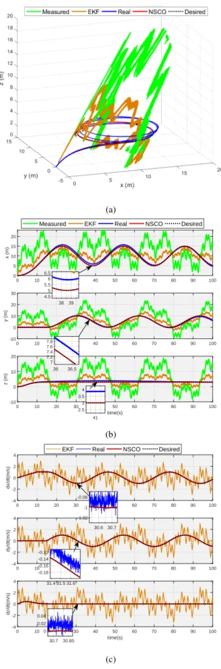
Reference trajectory:Tracking desired position trajectory is studied. The desired trajectory consists of takeoff and a circle with the radius 5m, velocity 1m/s and altitude 3m, which is shown in Fig. 5.

The NSCO (5) estimates the position and velocity from the contaminated position and acceleration measurements. Controllers (17) and (24) are adopted to drive the UAV to track the reference trajectory. The parameters of NSCOs are: αi,3 = 0.5, ki,1 = 0.5, ki,2 = 0.2, ki,3 = 10, 1/εi = 4, i = 1,2,3. The controller gains are: kp1 = 3.2, kp2 = 5,

(a)

0 10 20 30 40 50 60 70 80 90 100

0 5 10 15 20

x (m)

Measured EKF Real NSCO Desired

0 10 20 30 40 50 60 70 80 90 100

-10 0 10 20 30

y (m)

0 10 20 30 40 50 60 70 80 90 100

time(s)

-10 0 10 20

z (m)

38 39

4.5 5 5.5 6 6.5

36 36.5

7 7.2 7.4 7.6 7.8

41 2.5

3 3.5 4

(b)

0 10 20 30 40 50 60 70 80 90 100

-4 -2 0 2 4

dx/dt(m/s)

EKF Real NSCO Desired

0 10 20 30 40 50 60 70 80 90 100

-4 -2 0 2 4

dy/dt(m/s)

0 10 20 30 40 50 60 70 80 90 100

time(s)

-4 -2 0 2 4

dz/dt(m/s)

30.6 30.7

-1.02 -1 -0.98

31.4 31.5 31.6 -0.18 -0.16 -0.14 -0.12

30.7 30.85

0 0.02 0.04

(c)

ka1= 2.6,ka2= 3.5.

The NSCO provides the estimations of the position and velocity, which are replaced into the controller. Now, the N-SCO performance is studied through the behavior of estimated position and velocity, and compared with the estimations by the EKF given in [17]. The estimations of the states by the EKF consider the same conditions.

Fig. 5(a) displays the estimated trajectories by the NSCO and EKF. In addition, the estimation comparisons of the three-direction positions are shown in Fig. 5(b): The sensor errors of position measurements are 20m. The errors by the NSCO are less than 1m, while the up-boundness of the estimate errors by the EKF is 6m for all the positions. The large measurement errors and stochastic noises are rejected sufficiently by the NSCO. Importantly, even in the long-time flight (1000s), no drift phenomenon happened. However, comparing to the NSCO, the larger position estimation errors exist by the EKF, and the EKF can’t restrain efficiently the effect of stochastic non-Gaussian noise. Fig. 5(c) illustrates the comparison of velocity estimations between the NSCO and the EKF, where the velocity estimations from the NSCO showed the smaller error estimations.

Importantly, we found that the rules of NSCO parameters selection (Remark 2) are confirmed by tuning parameters of NSCO in the experiment: 1) For the parameterε∈(0,1): on the one hand, ifεdecreases, the estimation speed will increase, and the low-pass frequency bandwidth will become larger; on the other hand, ε increases, much noise will be rejected. 2) The smallerk1>0can reduce the adverse effect of the larger

position measurement error, and the estimate precisions will be improved. 3) The selection of smallerα3∈(0,1)can improve

the estimate precisions, and relatively largeα3can reject much

high-frequency noise.

VI. CONCLUSION

A NSCO has been developed. It can reject the large sensor error in position and also can estimate the unknown velocity in spite of the existence of stochastic non-Gaussian noise. The proposed scheme demonstrated by experiment, that it succeeded in rejecting the large measurement error in position, and in estimating the unknown flying velocity. The merits of the presented NSCO include its synchronous signal estimation and measurement error reduction, sufficient stochastic non-Gaussian noise rejection and no drift phenomenon.

APPENDIX

Proof of Theorem 1: The error system between the NSCO (5) and the derivatives of a01(t)is given by:

˙

e1 = e2; e˙2=e3;

ε4e˙3 = −k1|ε(e1−d1(t))|α1sign(e1−d1(t))

−k2ε2(e2+a02(t)) α2

sign(e2+a02(t))

−k3|e3−d3(t)|

α3_sign(e

3−d3(t))

−ε4a˙03(t) (25)

Eq. (25) can be rewritten as

dεe1

dt/ε = ε

2_e 2;

dε2_e 2

dt/ε =ε

3_e 2

dε3_e 3

dt/ε = −k1|εe1−εd1(t)|

α1_sign(e

1−d1(t))

−k2ε2e2+ε2a02(t) α2

sign(e2+a02(t))

− k3

ε3α3

ε3e3−ε3d3(t) α3

sign(e3−d3(t))

−ε4a˙03(t) (26)

Selecting the coordinate transform

τ = t/ε;zi(τ) =εiei;z=

[

z1 z2 z3

]T

;

di(τ) = εidi(t), i= 1,3;d2(τ) =ε2a02(t) ;

d4(τ) = ε4a˙03(t) (27)

we obtainz= Ξ(ε)e, and Eq. (26) can be written as

dz1

dτ = z2; dz2

dτ =z3; dz3

dτ = −

2

∑

i=1

ki|zi|

αi_sign(z

i)

− k3

ε3α3 |(z3)|

α3_sign(z

3) +g(τ, z(τ)) (28)

where

g(τ, z(τ))

= −k1

{

z1−d1(τ) α1

sign(z1−d1(τ)

)

− |z1|

α1_sign(z 1)}

−k2

{

z2+d2(τ) α2

sign(z2+d2(τ)

)

− |z2|

α2_sign(z

2)} −d4(τ)

− k3

ε3α3

{

z3−d3(τ) α3

sign(z3−d3(τ)

)

− |z3|

α3_sign(z

3)} (29)

Since the nonlinear contraction mapping |xρi−_xρi| ≤ 21−ρi|_x−_x|ρi_{, ρ}

i∈(0,1], we obtain

δ = sup

(τ,z)_∈R4|

g(τ, z(τ))|

≤

2

∑

i=1

21−αi_k

iLαiiε

iαi_+ε4_L

a+ 21−α3k3Lα33

≤ ερδ0+ 21−α3k3Lα33 (30)

where, δ0 = 2

∑

i=1

21−αi_k

iLαii + La, and ρ =

mini_∈{1,2,3_}{min{4, iαi}}=α1.

From Proposition 8.1 in [18], Theorem 5.2 in [19] and Eq. (30), for system (28), there exist positive constants µ and

Γ (z(0)), such that, for∀τ∈[Γ (z(0)),∞),

∥z(τ)∥ ≤µδγ≤µ(εα1_δ

0+ 21−α3k3Lα33) γ

whereµis a constant defined in Theorem 5.2 [19]. Therefore, from coordinate transformation (27), we obtain

∥ εe1 ε2e2 ε3e3 ∥ ≤µ(εα1δ0+ 21−α3k3Lα33)

γ ₍₃₂₎

for ∀t ∈[εΓ (Ξ(ε)e(0)),∞). Thus, the following inequality

holds:

|ei| ≤L(δdi)γ, i= 1,2,3,∀t∈[εΓ (Ξ(ε)e(0)),∞) (33)

where L=µδ₀γ;δdi =εα1−

i

γ +2

1−α_3k

3Lα33

δ0 ε

−i

γ_,i= 1,2,3_.

If ε∈(0,1)andL3<

(

1−εα1 21−α3k3δ0

)1

α3

, then

0< εα1₊2 1₋α3

δ0

k3Lα33 <1 (34)

Furthermore, from Theorems 4.3 and 5.2 in [19], γ can be chosen to be arbitrarily large. Hence, the requirement that γ lies on

γ >max {

4 logε

log(εα1₊21−α3 δ0 k3L

α3 3 )

,1 }

(35)

is not restrictive. Therefore,

γlog(εα1₊2 1−α3

δ0

k3Lα33)<4 logε (36)

i.e.,

εα1₊2 1−α3

δ0

k3Lα33 < ε 4

γ ₍₃₇₎

From Eq. (35),γ >4holds. Therefore, fromε∈(0,1), we can obtain ε4γ _{< ε}

i

γ_{,i= 1,2,3. Then}

δdi =εα1−

i

γ ₊2

1−α3

δ0

k3Lα33ε−

i

γ _{<1 (38)}

where i = 1,2,3. The choice of γ leads to γ > 1 in (33) which implies that for δdi ∈ (0,1), the ultimate bound (33) on the estimation error is of higher order than the perturba-tion. Consequently, the NSCO leads to perform rejection of persistent disturbances.

Furthermore, assume there is no sensor error in signala3(t),

i.e, a3(t) =a03(t)or L3= 0, then (33) can be written as

|ei| ≤Lεα1γ−i, i= 1,2,3,∀t∈[εΓ (Ξ(ε)e(0)),∞) (39)

We know that α1γ −i > 1, i = 1,2,3. In fact, from

Theorems 4.3 and 5.2 in [19],γcan be chosen to be arbitrarily large, and

γ >max {

4

α1

,1 }

= 4

α1

(40)

is not restrictive. Accordingly, fori= 1,2,3, we can obtain

α1γ−i >1 (41)

It implies that, for ε∈ (0,1), the ultimate bound (39) on the estimation error is of higher order than the perturbation.

For arbitrary ε ∈(0,1), from the Routh-Hurwitz Stability Criterion,s3₊ k3

ε3α₃s2+k2s+k1is Hurwitz ifk1>0,k3>0,

k2> ε3α3k1/k3. This concludes the proof.

REFERENCES

[1] D. Odijk, N. Nadarajah, S. Zaminpardaz, P.J. G. Teunissen. GPS, Galileo, QZSS and IRNSS differential ISBs: estimation and application, GPS Solutions, vol. 21, no. 2, 439-450, Apr. 2017.

[2] M.F. Abdel-Hafez. Detection of bias in GPS satellites’ measure-ments: A probability ratio test formulation,IEEE Trans. Control Syst. Technol., Vol. 22, No. 3, 1166-1173, 2014.

[3] M.S. Golsorkhi, D.D.C. Lu, J.M. Guerrero. A GPS-Based Decentralized Control Method for Islanded Microgrids, IEEE Transactions on Power Electronics, vol. 32, no. 2, 1615-1625, Feb. 2017.

[4] L.R.G. Carrillo, I. Fantoni, and E. Rondon. Three-dimensional position and velocity regulation of a quad-rotorcraft using op-tical flow, IEEE Trans. Aerosp. Electron. Syst., vol. 51, no. 1, 358-371, 2015.

[5] M. Lungu R. Lungu. Design of full-order observers for Systems with unknown inputs by using the eigenstructure assignment.

Asian J. Control, vol. 16, no. 5, pp. 1470-1481, 2014.

[6] Z. Pu, R. Yuan, J. Yi, X. Tan. A class of adaptive extended state observers for nonlinear disturbed systems,IEEE Trans. Ind. Electron., vol. 62, no. 9, 5858-5869, Sept. 2015.

[7] M. Lungu, R. Lungu. Reduced-order multiple observer for aircraft state estimation during landing.Applied Mechanics and Materials, vol. 841, pp. 253-259, 2016.

[8] M.K. Jalloul, M.A. Al-Alaoui. Design of recursive digital in-tegrators and differentiators using particle swarm optimization,

Int. J. Circ. Theor. App., vol. 44, no. 5, pp. 948-967, 2016.

[9] A. Aggarwal, T.K. Rawat, D.K. Upadhyay. Optimal design of L1-norm based IIR digital differentiators and integrators using the bat algorithm, IET Signal Processing, vol. 11, no. 1, pp. 26-35, Feb. 2017.

[10] J.M. Hansen , T.A. Johansen, N. Sokolova, T.I. Fossen. Nonlin-ear Observer for Tightly Coupled Integrated Inertial Navigation Aided by RTK-GNSS Measurements,IEEE Trans. Control Syst. Technol., DOI: 10.1109/TCST.2017.2785840

[11] X. Wang, B. Shirinzadeh, and M.H. Ang,Jr. Nonlinear double-integral observer and application to quadrotor aircraft, IEEE Trans. Ind. Electron., vol. 62, no. 2, 1189-1200, 2015.

[12] R.H. Rogne, T.H. Bryne, T.I. Fossen, T.A. Johansen. Redundant MEMS-based inertial navigation using nonlinear Observers, J. Dyn. Sys., Meas., Control, vol. 140, no. 7, 071001 1-7, Jul. 2018.

[13] D.A. Mercado, G. Flores, P. Castillo1, J. Escareno, and R. Lozano1. GPS/INS/Optic flow data fusion for position and ve-locity estimation, 2013 International Conference on Unmanned Aircraft Systems (ICUAS), Grand Hyatt Atlanta, Atlanta, GA, May 28-31, 2013, 486-491.

[14] Y. Kim, J. An, J. Lee. Robust navigational system for a trans-porter using GPS/INS fusion, IEEE Trans. Ind. Electron., vol. 65, no. 4, 3346-3354, Apr. 2018.

[15] M.A.K. Jaradat, M.F. Abdel-Hafez. Non-linear autoregressive delay-dependent INS/GPS navigation system using neural net-works, IEEE Sensors J., vol. 17, no. 4, pp. 1105-1115, Feb. 2017.

[16] F. Auger, M. Hilairet, J.M. Guerrero, E. Monmasson. Industrial applications of the Kalman filter: A Review, IEEE Trans. Ind. Electron., vol. 60, no. 12, 5458-5471, Dec. 2013.

[17] L. Idkhajine, E. Monmasson, A. Maalouf. Fully FPGA-based sensorless control for synchronous AC drive Using an Extended Kalman filter,IEEE Trans. Ind. Electron., vol. 59, no. 10, 3908-3918, Oct. 2012.

[18] S.P. Bhat and D.S. Bernstein. Geometric homogeneity with applications to finite-time stability,Math. Control, Signals, Syst., vol. 17, no. 2, 101-127, Jun. 2005.

[19] S.P. Bhat and D.S. Bernstein. Finite-time stability of continuous autonomous systems, Siam J. Control Optim., vol. 38, no. 3, 751-766, Mar. 2000.

[21] A. Tayebi and S. McGilvray, Attitude stabilization of a VTOL quadrotor aircraft,”IEEE Trans. Control Syst. Technol., vol. 14, no. 3, pp. 562-571, May 2006.

[22] S. Islam, P.X. Liu, A.E. Saddik. Observer-based adaptive output feedback control for miniature aerial vehicle,IEEE Trans. Ind. Electron., vol. 65, no. 1, 470-477, Jan. 2018.

[23] F. Chen, R. Jiang, K. Zhang, B. Jiang, G. Tao. Robust backstep-ping sliding-mode control and observer-based fault estimation for a quadrotor UAV,IEEE Trans. Ind. Electron., vol. 63, no. 8, 5044-5056, Aug. 2016.

[24] M. Lungu, R. Lungu, C. Rotaru. New systems for identification, estimation and adaptive control of the aircrafts movement.

Studies in Informatics and Control, vol. 20, no. 3, pp. 273-284, 2011.

[25] K. Sebesta and N. Boizot. A real-time adaptive high-gain EKF, applied to a quadcopter inertial navigation system,IEEE Trans. Ind. Electron., vol. 61, no. 1, pp. 495-503, Jan. 2014.

[26] T. Hamela and R. Mahony. Image based visual servo control for

a class of aerial robotic system,Automatica, vol. 43, no. 11, pp. 1976-1983, Nov. 2007.

[27] N. Guenard, T. Hamel, and R. Mahony. A practical visual servo control for an unmanned aerial vehicle,IEEE Trans. Robot., vol. 24, no. 2, pp. 331-340, Apr. 2008.

[28] A. Levant. High-order sliding modes, differentiation and output-feedback control,Int. J. of Control, vol. 76, no. 9/10, 924-941, 2003.

[29] R. Baltes, A. Schultschik, O. Farle, and R. Dyczij-Edlinger. A finite-element-based fast frequency sweep framework including excitation by frequency-dependent waveguide mode patterns,

IEEE Trans. Microw. Theory Techn., vol. 65, no. 7, pp. 2249-2260, Jul. 2017.