University of Warwick institutional repository: http://go.warwick.ac.uk/wrap
A Thesis Submitted for the Degree of PhD at the University of Warwick
http://go.warwick.ac.uk/wrap/3903
This thesis is made available online and is protected by original copyright.
Please scroll down to view the document itself.
Statistical Description and Modelling of Fusion Plasma
Edge Turbulence
by
Joseph Michael Dewhurst
Thesis
Submitted to the University of Warwick
for the degree of
Doctor of Philosophy
Contents
List of Tables v
List of Figures vi
Acknowledgments xiii
Abstract xv
Chapter 1 Introduction 1
1.1 Thermonuclear fusion . . . 1
1.2 Plasma . . . 3
1.3 Charged particle motion in electromagnetic fields . . . 4
1.4 Kinetic description of plasma . . . 6
1.5 Fluid description of plasma . . . 7
1.6 Magnetohydrodynamic equilibrium . . . 8
1.6.1 Stellarator . . . 10
1.6.2 Tokamak . . . 11
1.6.3 Edge plasma . . . 12
1.7 Classical transport . . . 15
1.7.1 Classical transport . . . 15
1.7.2 Neoclassical transport . . . 16
1.8.1 Turbulence . . . 17
1.8.2 Wave-wave interaction . . . 19
1.8.3 Plasma instabilities . . . 20
1.9 Outline . . . 22
Chapter 2 Statistical description of LHD and MAST edge turbulence 24 2.1 Introduction . . . 24
2.2 Statistical analysis background . . . 26
2.2.1 Probability density function . . . 26
2.2.2 Correlation . . . 27
2.2.3 Power spectral density . . . 27
2.3 Absolute moment analysis . . . 28
2.3.1 Turbulence and fractals . . . 28
2.3.2 Langmuir probes . . . 29
2.3.3 Scaling of absolute moments . . . 30
2.3.4 Synthetic time series . . . 31
2.4 LHD scaling . . . 33
2.4.1 LHD data . . . 33
2.4.2 Scaling properties . . . 35
2.5 MAST scaling . . . 41
2.6 Probability density function . . . 43
2.6.1 LHD . . . 43
2.6.2 MAST . . . 47
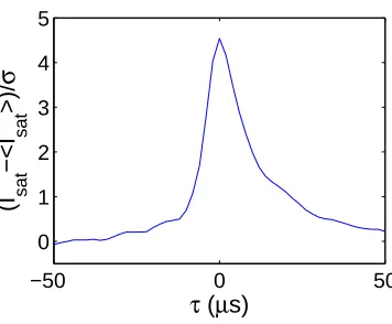
2.7 Average temporal shape of large bursts . . . 48
2.8 Discussion . . . 50
2.9 Conclusions . . . 53
3.2 Derivation of Hasegawa Wakatani equations . . . 56
3.3 Numerical methods . . . 61
3.3.1 Dissipation . . . 61
3.3.2 Spatial discretisation . . . 62
3.3.3 Temporal discretisation . . . 62
3.3.4 Poisson’s equation . . . 63
3.4 Testing the HAWK code . . . 64
3.4.1 Linear dispersion relation . . . 64
3.4.2 Energy and enstrophy conservation . . . 67
3.5 HAWK simulation . . . 68
3.6 Zonal flows . . . 70
3.6.1 Zonal flow damping . . . 72
3.6.2 Zonal flows as transport barriers . . . 72
3.7 Non-uniform magnetic field strength . . . 75
3.7.1 Propagation of nonlinear structures . . . 77
3.7.2 Computations in polar coordinates . . . 80
Chapter 4 Statistical properties of drift wave turbulence 81 4.1 Introduction . . . 81
4.2 Turbulent flux PDF . . . 81
4.2.1 Varyingκ . . . 83
4.2.2 Varyingα . . . 84
4.2.3 VaryingC . . . 85
4.3 Structure function analysis . . . 87
4.4 Higher order spectra . . . 90
4.4.1 Bispectral analysis of HAWK data . . . 91
Chapter 5 Test particle transport 97
5.1 Introduction . . . 97
5.2 Test particle evolution . . . 98
5.3 Non-uniform magnetic field strength . . . 100
5.3.1 Introduction . . . 100
5.3.2 Running diffusion coefficients . . . 101
5.3.3 Fick’s law . . . 102
5.3.4 Summary . . . 105
5.4 Zonal flow and finite Larmor radius . . . 106
5.4.1 Introduction . . . 106
5.4.2 Properties of the turbulence . . . 107
5.4.3 Test particle transport . . . 110
5.4.4 Test particle displacements . . . 110
5.4.5 Test particle diffusion . . . 111
5.4.6 Larmor radius dependence . . . 114
5.4.7 Discussion . . . 116
5.4.8 Summary . . . 118
Chapter 6 Summary and future work 119 6.1 Further work . . . 120
6.1.1 Analysis of experimental data . . . 121
List of Tables
1.1 Typical parameters for LHD and MAST. . . 13
List of Figures
1.1 Cross sections for various fusion reactions [Wesson, 2004]. . . 2 1.2 Origin of the diamagnetic drift [Wesson, 2004]. . . 6 1.3 The torus. . . 9 1.4 Principle of the tokamak [Pecseli, 2009] (left) and stellarator [ENS, 2009]
(right). . . 10 1.5 The Large Helical Device (LHD) stellarator [NIFS, 2009]. . . 10 1.6 External (left) and internal (right) photographs of the Mega-Amp
Spher-ical Tokamak (MAST) [CCFE, 2009]. . . 11 1.7 Simplified magnetic field structure of a diverted tokamak (left) and
he-liotron type stellarator (right). . . 14 1.8 Cartoon of the energy spectrum E(k) expected in 3-dimensional (left)
and 2-dimensional (right) hydrodynamic turbulence. . . 18 1.9 The physics of the drift wave. Adapted from [Chen, 1984]. . . 21
2.2 (a) Absolute moments of order m = 2 and m = 4 and (b) derived scaling exponentsζ(m)for random Gaussian noise added to a sine wave 100 000 points long. Moments m = 1 and m = 3 are omitted from (a) for clarity. The dashed line in (a) indicates the period of the sine wave,T = 100points. The amplitude of the sine wave relative to to the standard deviation of the Gaussian noise,A=a/σ, is varied. . . 32 2.3 (a) Location of the Langmuir probe array within LHD [Ohno et al.,
2006b]. (b) Location of probes within probe array [Ohno et al., 2006b]. 34 2.4 Visible light image of LHD discharge 44190. . . 34 2.5 Isat signals for LHD plasma 44190: (a) tip 16; (b) tip 17; (c) tip 18. . . 35
2.6 Absolute moments of order1≤m≤4(left) and power spectral density (right) for LHD plasma 44190: (a) and (b) tip 16; (c) and (d) tip 17; (e) and (f) tip 18. The dashed line on each plot of absolute moments corresponds to the reciprocal of the frequency of the coherent mode marked on the power spectral density. . . 36 2.7 Autocorrelation function for LHD plasma 44190 before (left) and after
(right) bandstop filtering to remove coherent modes: (a) and (b) tip 16, (c) and (d) tip 17, (e) and (f) tip 18. The horizontal dashed line at 0.05 is used to define τA. . . 38
2.8 Absolute moments of order1 ≤m≤4 (left) and derived scaling expo-nents ζ(m) (right) for Isat signal of LHD plasma 44190 with bandstop
filters applied to remove coherent modes: (a) and (b) tip 16; (c) and (d) tip 17; (e) and (f) tip 18. . . 40 2.9 Isat signal from MAST plasma 14222. . . 41
2.12 Probability density functions P(δIsat, τ) of the filtered data forτ = 4µs
(left) andτ = 64µs (right) normalised to, σ, the standard deviation of δIsat(t, τ): (a) and (b) tip 16; (c) and (d) tip 17; (e) and (f) tip 18.
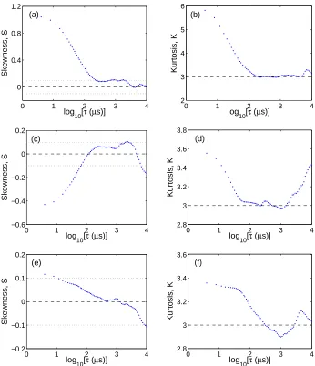
Gaussian PDFs (dashed line) are plotted for comparison. In (a) we show Fr´echet (red) and Gumbel (green) fits. . . 45 2.13 Measured skewness and kurtosis as a function of τ for all three tips in
LHD plasma 44190, using filtered data for: (a) and (b) tip 16; (c) and (d) tip 17; (e) and (f) tip 18. Horizontal dashed lines mark Gaussian values for skewness (S = 0) and kurtosis (K = 3) respectively. Horizontal dotted lines mark the threshold|S|= 0.1 for the skewness time scaleτS. 46 2.14 Probability density functions P(δIsat, τ) of the MAST data for (a)τ =
2µs and (b) τ = 64µs normalised to, σ, the standard deviation of
δIsat(t, τ). Gaussian PDFs (dashed line) are plotted for comparison.
In (a) we show Fr´echet fit (red) and in (b) Gumbel fit (green). . . 47 2.15 Measured skewness and kurtosis as a function of τ for MAST plasma
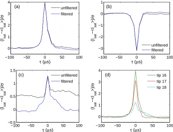
14222. Horizontal dashed lines mark Gaussian values for skewness (S= 0) and kurtosis (K = 3) respectively. . . 48 2.16 Average burst shapes calculated by conditional averaging for LHD plasma
44190 before and after filtering: (a) tip 16; (b) tip 17; (c) tip 18; (d) comparison. . . 49 2.17 Average burst shape calculated by conditional averaging for MAST plasma
14222. . . 50
3.1 Physical setting of the Hasegawa-Wakatani equations. The shaded square represents the computational domain. . . 56 3.2 (a) Real and (b) imaginary parts of the solution to the HW analytical
dispersion relation (equation 3.33) withα= 0.5 andκ= 1.0. . . 66 3.3 Linear growth rate measured in the HAWK code using parametersα =
3.4 (a) Energy and (b) enstrophy conservation in the HAWK code: equations 3.43 and 3.44. . . 68 3.5 Snapshots of densitynand potentialφand time series of energyE taken
from the HAWK code. The dashed lines in theE time series correspond to the times at which snapshots are taken. . . 69 3.6 Snapshots of densitynand potentialφand time series of energyE, zonal
energy hEi and non-zonal energyE˜ taken from a HAWK simulation of the ZHW model (equations 3.49 and 3.50). The dashed lines in the E time series correspond to the times at which snapshots are taken. . . . 71 3.7 Snapshots of density n and potential φ and time series of energy E,
zonal energyhEiand non-zonal energyE˜ taken from a simulation of the DZHW model (equations 3.49 and 3.50 with the constraint of equation 3.54). The dashed lines in theE time series correspond to the times at which snapshots are taken. . . 73 3.8 Density profilen0 relaxation with (bottom) and without (top) zonal flows. 74
3.9 Contours of potentialφin the quasi-stationary saturated turbulent state of the CHW system for different values ofC =−∂lnB/∂x. . . 77 3.10 Radial evolution of density nof nonlinear structures for different values
of C = −∂lnB/∂x. The directions of the gradients of background magnetic field and density are opposed for negativeCand coincident for positiveC. . . 78 3.11 Radial ux and poloidal uy velocity components of positive amplitude
nonlinear structures shown in Fig. 3.10 for different values ofC. . . 78 3.12 Snapshot of density fluctuations from HAWK simulation of the CHW
4.1 (a) PDF of point-wise radial density fluxΓn=nvx for the base case, as described in the text. The dashed lines are the PDFs calculated using equations 4.2 and 4.3 and probe data from the simulation. (b) PDF of point-wise densityn, radial velocityvxand potentialφfor the base case. The dashed lines are Gaussian fits to the data. . . 82 4.2 (a) PDF of point-wise radial density flux Γn = nvx for different values
ofκ. The dashed lines are the PDFs calculated using equations 4.2 and 4.3 and probe data from the simulation. (b) Relative phase between n andvx, for different values ofκ. (c) Average total flux Γn0 for different
κ. (d) rms values ofn andvx fluctuations. . . 84 4.3 (a) PDF of point-wise radial density flux Γn = nvx for different values
ofα. The dashed lines are the PDFs calculated using equations 4.2 and 4.3 and probe data from the simulation. (b) Relative phase between n andvx, for different values ofα. (c) Average total fluxΓn0 for different
α. (d) rms values ofn andvx fluctuations. . . 85 4.4 (a) PDFs and (b) skewness of PDFs of the point-wise radial density flux
Γn=nvx for different values of C. The dashed lines over the PDFs are the PDFs calculated using equations 4.2 and 4.3 and probe data from the simulation. (c) Skewness and kurtosis of PDFs of point-wise density n, radial velocityvx and potentialφ. (d) Relative phase between nand vx, and between n and φ, for different values of C. (e) Average total fluxΓn0 for differentC. (f) rms values of nandvx fluctuations. . . 86
4.5 Structure function analysis of density data taken from the HAWK code. (a) Structure functions Sm of order m = 1 to m = 8 as a function of d for C = −0.3. (b) Extended self-similarity (ESS) analysis: structure functions Sm as a function ofS3 for C =−0.3. (c) Scaling exponents
4.6 Structure function analysis of velocity data taken from the HAWK code: scaling exponentsζ(m)calculated using ESS structure functions for dif-ferent values ofC. . . 89 4.7 Bicoherence calculated using multiple snapshots of potential from a
HAWK simulation of the HW equations. . . 91 4.8 Nonlinear transfer functions for different values ofC. . . 93 4.9 Nonlinear transfer functions for the HW and ZHW models. . . 94 4.10 Nonlinear transfer functions for the HW and ZHW models. The dashed
lines indicate the zonal flow contribution (ky = 0). . . 96 5.1 Plots of running diffusion coefficient (a)Dx, and (b)Dy versus time for
different values ofC. . . 102 5.2 Plots ofX2/t0.45 andY2/t1.7 versus time for C =−0.5showing
subd-iffusion inx and superdiffusion iny. . . 103 5.3 (a) Time independent diffusion coefficientsDx andDy for different
val-ues ofC. (b) Average radial density fluxΓn0and(κ−C)Dx for different values ofC. . . 104 5.4 Normalised correlation between fluid potential vorticityζ0 att= 0, and
fluid potential vorticityζ at time t, for different values ofC. . . 105 5.5 Snapshot of potentialφin the saturated quasi-stationary turbulent state
for three related models: (left) HW defined by equations 3.19 and 3.20 where zonal flows are damped; (centre) ZHW defined by equations 3.49 and 3.20 allowing the self-generation of zonal flows; (right) intermediate state DZHW where total kinetic energy of zonal flows is set equal to that of non-zonal drift wave turbulence at each time step. . . 107 5.6 Weiss field, Q, calculated from data in figure 5.5: (left) HW; (centre)
5.8 PDFs of jumps∆x(left) and ∆y (right) made by particles forρ= 0 in the HW, ZHW and intermediate DZHW cases. . . 111 5.9 Test particle diffusion: (a) and (b)X2/2tandY2/2tversus time for HW
case showing normal diffusion; (c) and (d) X2/(2t)0.8 and Y2/(2t)1.55
versus time for ZHW case demonstrating subdiffusion inx and superdif-fusion in y; (e) and (f) X2/2t and Y2/2t versus time for intermediate DZHW turbulence case showing normal diffusion. . . 112 5.10 Value of diffusion coefficients Dx and Dy at the end of the simulation
(t= 2500normalised time units) as a function ofρ: (a) and (b) HW case; (c) and (d) ZHW case; (e) and (f) intermediate DZHW turbulence case. Crosses indicate results when all the test particle share the same Larmor radius ρ; circles indicate results when the Larmor radii are distributed around a most probable valueρ. . . 115
Acknowledgments
I would like to thank my supervisor Bogdan Hnat for his help, support and flexibility during my time at Warwick. I am very grateful to Richard Dendy for his insight, advice and encouragement over the past three and a half years.
Thank you S Masuzaki, T Morisaki, N Ohno, H Tsuchiya and A Komori for the friend-liness and hospitality which made my visit to NIFS such a great experience.
Thank you to everyone at CFSA, especially Francis Casson and Chris Brady for help with computational problems.
I’d like to acknowledge the continuing support and advice from my parents and grand-mother. To my in-laws, the Nakamuras, I am extremely grateful.
Abstract
In tokamaks, heat and particle fluxes reaching the wall are often bursty and intermittent and understanding this behaviour is vital for the design of future reactors. Plasma edge turbulence plays an important role, its quantitative characterisation and modelling under different operating regimes is therefore an important area of research.
Ion saturation current (Isat) measurements made in the edge region of the Large
Helical Device (LHD) and Mega-Amp Spherical Tokamak (MAST) are analysed. Ab-solute moment analysis is used to quantify properties on different temporal scales of the measured signals, which are bursty and intermittent. In all data sets, two regions of power-law scaling are found, with the temporal scale τ ≈ 40µs separating the two regimes. A monotonic relationship between connection length and skewness of the probability density function is found for LHD.
A new numerical code, ‘HAWK,’ which solves the Hasegawa-Wakatani (HW) equations is presented. The HAWK code is successfully tested and used to study the HW model and modifications. The curvature-Hasegawa-Wakatani (CHW) equations in-clude a magnetic field strength inhomogeneity,C=−∂lnB/∂x. The zonal-Hasegawa-Wakatani (ZHW) equations allow the self-generation of zonal flows. The statistical properties of the turbulent fluctuations produced by the HW model and variations thereof are studied. In particular, the probability density function of E ×B density flux Γn = −n∂φ/∂y, structure functions, the bispectrum and transfer functions are investigated.
Chapter 1
Introduction
1.1
Thermonuclear fusion
The world’s energy requirements are rapidly increasing as the global population rises and nations become more industrialised. With growing concerns over the finite size of the world’s fossil fuel supplies and their contribution to climate change, the need for a clean, safe, carbon-neutral and politically-neutral form of electricity generation is clear. Controlled thermonuclear fusion has long been recognised as an ideal solution.
Fusion is the process that powers the Sun. During the reaction, nuclei fuse together and the mass of the reaction products is less than the mass of the reactants. Due to this small mass loss, and Einstein’s famous mass-energy equivalenceE =mc2, energy is released. The fusion of nuclei relies on the nuclear force, which is attractive on very small spatial scales; nuclei, however, are positively charged and experience mutual electrostatic repulsion. Thus for the fusion reaction to proceed, an electrostatic potential barrier must be overcome.
Figure 1.1: Cross sections for various fusion reactions [Wesson, 2004].
100keV. The reaction is as follows,
D+T→α(3.5MeV) +n(14MeV) ; (1.1)
D and T nuclei fuse together creating an alpha particle and a neutron, and releasing 17.5 MeV of energy. Deuterium and tritium are relatively abundant–deuterium is found in sea water while tritium can be bred from lithium–and will therefore be the fuel of choice for the first generation of fusion reactors. It is important to note that, unlike in nuclear fission, the fusion reaction cannot lead to a catastrophic runaway event and produces little radioactive waste. In fact, small quantities of short-lived radioactive waste would be produced indirectly due to the activation of the device by neutron bombardment.
Thermonuclear fusion occurs when the fuel is heated sufficiently so that the ther-mal velocities of the particles are large enough to produce the required fusion reactions. The optimum temperature for D-T thermonuclear fusion is around 30keV, less than the 100keV peak in figure 1.1 since a significant fraction of the fusion reactions can occur in the high energy tail of the Maxwellian [Wesson, 2004]. At such high temperatures, the fuel will be a fully ionised plasma.
plasma andP is the rate of energy loss. The plasma is said to reach ignition when all energy losses are balanced by alpha particle heating and no external energy inputs are needed to maintain the fusion reaction. The relevant criterion was derived by Lawson and expressed in terms of nτe. At a temperature of 30keV, the Lawson criterion for ignition is
nτe>1.5×10²⁰sm−3 . (1.2) There are generally two approaches to satisfying this inequality: inertial confinement and magnetic confinement. Inertial confinement involves the rapid compression of small fuel pellets using high powered lasers, aiming for extremely high values ofn and short τe. Magnetic confinement, which this thesis is concerned with, takes advantage of the charge of plasma particles and attempts to design a magnetic field to confine plasma at relatively lownand for long τe.
1.2
Plasma
A plasma is an ionised gas or, more accurately, “a quasi-neutral collection of ions and electrons which exhibits collective behaviour” [Chen, 1984]. In a plasma, electrons are much more mobile than ions due to their lower mass. Thus any charge imbalance is quickly screened out by the rapid movement of electrons, so that the bulk of the plasma can be considered neutral; this is quasi-neutrality. The length scale over which charge imbalance is screened out is called the Debye length,
λD =
ǫ0Te
ne2
1
2
, (1.3)
1/ωpe, where
ωpe=
ne2
meǫo
12
=
Te me
12
1
λD
, (1.4)
is the plasma frequency. For quasi-neutralityλD must be small compared to the system size and 1/ωpe must be small compared to the collision time. Also, the plasma must be dense enough so that charge imbalance is screened effectively, this condition can be written,
nλ3D ≫1. (1.5)
This also ensures collective behaviour because it implies that plasma particles interact with a large number of others.
1.3
Charged particle motion in electromagnetic fields
On a small scale, a plasma can be understood as a soup of charged particles which react to, and generate electromagnetic fields. A particle of charge q and mass m, moving with velocity vin an electric fieldE and magnetic field B experiences a Lorentz force,
FL=q(E+v×B) . (1.6)
In the absence of an electric field and with a uniform magnetic field, the motion of the particle consists of a uniform velocity parallel toBand gyration perpendicular toBwith cyclotron (or gyro) frequency
ωc = qB
m , (1.7)
and Larmor radius
ρ= mv⊥
qB , (1.8)
where v⊥ is the component of velocity perpendicular to B. Thus the particle moves
along a helical path. This type of motion can be thought of as rapid gyration around a guiding centre which moves at constant velocity parallel toB. Such a circulating charge constitutes a current loop with magnetic moment,
µ= mv 2
⊥
If in addition to the magnetic field, the particle feels an electric field E, the guiding centre of the particle will drift with the so-called ‘E×B velocity’,
vE=
E×B
B2 , (1.10)
which is perpendicular to bothE andB. TheE×B velocity is the most fundamental of the plasma particle guiding centre drifts and plays a central role in the physics of magnetic confinement. Guiding centre drifts are created whenever plasma particles are subject to a forceF in the presence of a strong magnetic field B,
vF = 1
q
F×B
B2 . (1.11)
In the aboveE×B example, the particle experiences a forceF=qEdue to the electric field and equation 1.11 reduces to equation 1.10. Guiding centre drifts are also produced by non-uniform and time varying electromagnetic fields, for example the polarisation drift
vp is produced by a time varying electric field,
vp =±
1
ωcB dE
dt . (1.12)
One important plasma drift is the diamagnetic drift,
vd=−∇ p×B
qnB2 . (1.13)
This drift is not a particle drift: individual particles do not actually drift with vd. The diamagnetic drift is a fluid drift which arises due to the fluid-like nature of a plasma. The left hand side of figure 1.2 shows the orbits of plasma particles gyrating in a magnetic field. The plasma is inhomogeneous, with a density gradient pointing from right to left. As illustrated in the right hand side of figure 1.2, through any fixed volume of plasma there are more particles gyrating downwards than upwards. Thus there is a net drift of particles perpendicular to the magnetic field and density gradient.
Figure 1.2: Origin of the diamagnetic drift [Wesson, 2004].
1.4
Kinetic description of plasma
In most physically relevant situations it is not feasible to follow the individual motions of each plasma particle, and a statistical approach must be taken. The Vlasov equation treats plasma as a phase space continuum and describes the time evolution of the distribution function f(r,v, t) of a single plasma species in the presence of averaged electric and magnetic fields and in the absence of collisions. The Vlasov equation can be derived from first principles by considering individual particle motions in electric and magnetic fields [Clemmow and Dougherty, 1969]. When collisions are included, the equation becomes the Boltzmann equation,
df dt =
∂f
∂t +v· ∇f + q
m(E+v×B)· ∂f ∂v =
∂f ∂t
coll
=C(f, f) , (1.14)
1.5
Fluid description of plasma
It is often sufficient to describe a plasma by average quantities such as the number of particles of a given species per unit volume n, the mean velocity of these particles u
and the mean temperatureT. Such fluid equations were derived by Braginskii by taking moments of the Boltzmann equation [Braginskii, 1965]. In the two fluid model, ions and electrons are treated as two separate but interpenetrating fluids which interact with each other via electromagnetic fields. Each species has an equation for continuity
∂n
∂t +∇ ·(nu) = 0 , (1.15)
momentum
mn
∂
∂t +u· ∇
u=nq(E+u×B)− ∇p− ∇ ·Π +R , (1.16)
and energy
3 2n
∂
∂t +u· ∇
T =−p∇ ·u− ∇ ·q−Π :∇u+Q . (1.17)
Here,p=nT is the scalar pressure,Πis the traceless component of the pressure tensor,
R is the transfer of momentum from other species, q is the heat flux, Q is the heat exchange between species and the colon notation denotes the vector inner product. The plasma variables are coupled to electromagnetic fields which satisfy
∇ ·E = 0, (1.18)
∇ ·B = 0, (1.19)
∇ ×E = −∂B
∂t , (1.20)
∇ ×B = µ0J, (1.21)
Often, it is too computationally expensive to numerically solve the full two fluid Braginskii equations and many reduced models have been developed. In this thesis one such model, namely the Hasegawa-Wakatani model [Hasegawa and Wakatani, 1983], is extensively studied; see Chapter 3.
1.6
Magnetohydrodynamic equilibrium
One of the most successful ways of dealing with a plasma is treating it as a single electrically neutral conducting fluid; this is magnetohydrodynamics (MHD). The MHD equations can be derived by summing the Braginskii two fluid equations and thus rep-resent a further simplification to the description of a plasma. Ideal MHD assumes zero resistivity and the equations can be written,
∂ρ
∂t +∇ ·(ρu) = 0 , (1.22)
ρdu
dt =J×B− ∇p , (1.23)
E+u×B= 0 , (1.24)
whereρ is mass density [Dendy, 1990]. The equations are closed with an equation of state, Amp`ere’s law (equation 1.21) and Faraday’s law (equation 1.20).
MHD describes the large scale, bulk dynamics of a magnetised plasma and is thus used in the study of plasma equilibrium and stability. Using the force balance equation (equation 1.23), the conducting fluid will be at equilibrium when pressure gradients are balanced by the Lorentz force,
∇p=J×B . (1.25)
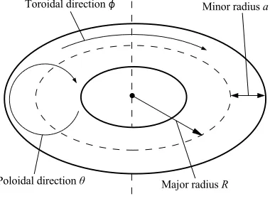
figure 1.3) and is characterised by the major radius R and minor radius a; the ratio R/a is called the aspect ratio. There are two directions around a torus: the long, toroidal way aroundφand the short, poloidal way aroundθ. Thinking naively, a plasma
Figure 1.3: The torus.
might be confined by driving a current through the hole of a torus, along the axis of symmetry thus producing a purely toroidal magnetic field. However, in such a situation the particles, following magnetic field lines, move in circles and therefore experience a centrifugal force. Such a force generates a guiding centre drift according to equation 1.11; a guiding centre drift is also produced by the non-uniform magnetic field strength (falling off with the major radius as1/R). These two drifts happen to be in the same direction and can be written together as
vd= m
q
vk2+1 2v
2
⊥
Rc×B R2
cB2
, (1.26)
where Rc is the radius of curvature and vk is the component of velocity parallel to
the magnetic field. Sincevd is charge dependent, its direction is opposite for ions and electrons: depending on the direction of the magnetic field, one species drifts up while the other drifts down. This generates an electric field and associatedE×B drift velocity in the direction perpendicular toB (equation 1.10) and the plasma particles are lost.
be short-circuited by rapid motion along field lines. There are two leading approaches to generating such a helical magnetic field: the tokamak and the stellarator; see figure 1.4.
Figure 1.4: Principle of the tokamak [Pecseli, 2009] (left) and stellarator [ENS, 2009] (right).
1.6.1 Stellarator
Figure 1.5: The Large Helical Device (LHD) stellarator [NIFS, 2009].
(LHD), located at the National Institute for Fusion Studies (NIFS) in Japan. LHD is a heliotron type stellarator with major radius R = 3.9m, minor radius a = 0.65m and superconducting field coils generating a magnetic field strength of typically 2.5T. Pictures of LHD are shown in figure 1.5; in the diagram on the right the helical shape of plasma can be seen in pink. The statistical analysis of experimental data taken from LHD forms part of Chapter 2 of this thesis.
1.6.2 Tokamak
Figure 1.6: External (left) and internal (right) photographs of the Mega-Amp Spherical Tokamak (MAST) [CCFE, 2009].
exper-iment with major radius R = 0.7m, minor radius a= 0.5 and a typical magnetic field strength of 0.5T; photographs are shown in figure 1.6. The shape of a typical MAST plasma can be seen in the right hand image: due to its low aspect ratio the plasma resembles a cored apple, rather than the doughnut shape associated with conventional tokamaks. The statistical analysis of experimental data from MAST and comparison with LHD forms Chapter 2 of this thesis.
The helicity of the magnetic field in a tokamak is quantified by the safety factor,
q= a
R Bφ
Bθ
. (1.27)
It is the number of times the magnetic field goes around toroidally per poloidal rotation. Stellarator physics typically uses1/q, the rotational transform. In tokamaks, the safety factor must be larger than one everywhere for stability. A safety factor less than one in the central region is associated with an MHD instability called the sawtooth oscillation. The ratio of plasma pressure to magnetic field pressure is an important quantityβ,
β = p
B2/2µ 0
. (1.28)
Commercial fusion reactors require β > 1% in order to be economically viable since the the fusion energy output scales with some power of p while the cost of the device depends mainly on the size of the magnetic field coils and scales with some power ofB [Chen, 1984].
Currently, the conventional tokamak is the most highly developed design, and on 21st November 2006 officials agreed to fund the creation of the ITER tokamak with the aim of demonstrating ignition for the first time in a magnetically confined plasma.
1.6.3 Edge plasma
LHD MAST Major radius,R 3.9m 0.7m Minor radius, a 0.65m 0.5m Plasma volume 30m3 8m3
Magnetic field strength 2.5T 0.5T Maximum discharge length 1 hour 1s
Table 1.1: Typical parameters for LHD and MAST.
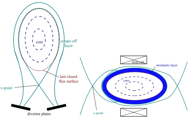
field lines which are connected to a divertor plate designed to handle large heat and particle fluxes, see figure 1.7. The closed field lines lie on ‘flux surfaces’ which, in a tokamak, form concentric tori. The last flux surface, radially, on which field lines are closed is called the ‘last closed flux surface’ (LCFS) and is commonly used to define the plasma edge. The region where field lines are open is referred to as the ‘scrape-off layer’ (SOL). The magnetic field geometry of stellarators is much more complex, the core region where field lines are closed is surrounded by an ‘ergodic layer’ where field lines wrap around the device to fill a volume. The edge region of a magnetically confined plasma is thus extremely complicated, containing large pressure gradients and complex magnetic geometry. Considerable numerical and theoretical effort is focused on trying to understand this region.
Figure 1.7: Simplified magnetic field structure of a diverted tokamak (left) and heliotron type stellarator (right).
1.7
Classical transport
1.7.1 Classical transport
So far in this introduction to magnetic confinement, collisions between plasma particles have been ignored. In the presence of collisions, particles experience stochastic forces and therefore perform random walks. Collisions cause a resistance to the flow of current and their effect can be understood in the context of MHD by introducing a resistivityη in equation 1.24,
E+u×B=ηJ. (1.29)
Taking the cross product withB and using equation 1.25 we obtain,
u⊥=
E×B
B2 −
η⊥
B2∇p . (1.30)
The first part of this velocity is theE×B drift that was seen earlier (equation 1.10). The second part is in the −∇p direction which is perpendicular to the confining magnetic field. Thus collisions cause a cross-field transport of plasma particles down the pressure gradient, i.e. collisions cause a reduction in the level of confinement. The flux associated with the velocity is
Γ⊥ =nu⊥=−
nη⊥
B2 ∇p=−
nη⊥T
B2 ∇n. (1.31)
This is like Fick’s law with diffusion coefficient
D⊥=
nη⊥T
B2 . (1.32)
This type of diffusion, caused by particle collisions, is referred to as classical diffusion or classical transport. In general a diffusion coefficient is of the form
D∼ (△x)
2
△t , (1.33)
1.7.2 Neoclassical transport
Geometric effects can cause an increase to the level of classical transport and this is referred to as neoclassical transport. For example, the magnetic mirror effect leads to neoclassical banana diffusion. Consider a charged particle in a magnetic fieldB. It can be shown that the magnetic momentµis constant forB varying slowly in space or time, in other words µ is adiabatically invariant. This leads to the magnetic mirror effect in the following way. By the definition of µ (equation 1.9), if the particle moves into a region of higherB,v⊥must increase in order to keepµconstant. Since the total energy
of the particle is constant and can be written as
E = mv 2
k
2 +
mv2
⊥
2 , (1.34)
an increase inv⊥ must be accompanied by a decrease invk. IfB is large enough, there
will come a point whenvk goes to zero and the particle is reflected. In tokamaks, the magnetic field strength falls off with the major radius as 1/R so that it is higher on the inboard side (near the axis of symmetry) than the outboard side. Thus particles moving in helical orbits experience an increase in magnetic field strength as they move from the outboard side to the inboard side. Particles with insufficient energy will be reflected and trapped in ‘banana orbits.’ Particles with sufficient energy to complete a full circuit around the tokamak are called passing particles. For the fraction of particles that are trapped in non-circulating ‘banana orbits,’ the step time △t and step size
△x of equation 1.33 become the banana orbit period and width respectively and thus diffusion is increased to neoclassical levels. Other neoclassical effects lead to plateau and Pfirsch-Schluter diffusion [Wesson, 2004].
1.8
Turbulent transport
extra transport is referred to as anomalous transport and is generally attributed to the presence turbulence generated by small scale instabilities.
1.8.1 Turbulence
Turbulence is a state of fluid motion characterised by unpredictability over a wide range of temporal and spacial scales. It is often referred to as the last great unsolved prob-lem of classical physics since the governing equations are deterministic and have been studied since the 19th century. Here, we introduce the phenomenology of hydrodynamic turbulence though this is not necessarily a good model for plasma turbulence.
In fluids dynamics a control parameter, called the Reynolds number, can be derived from a simple balance of nonlinear and dissipative terms in the momentum equation,
Re= vL
ν , (1.35)
where v is a typical fluid velocity, L is a typical length scale and ν is viscosity in the system. Transition from laminar to turbulent flow occurs for large values of Re in hydrodynamics. Similar parameters are often used for magnetised plasmas where one can define the Reynolds numberReand its magnetic counterpartRm[Biskamp, 1993]. It is important, however, to recognise that these constructs are not identical due to non-diffusive dissipation processes such as Landau damping which act on scales much smaller than the actual collisional dissipation.
energy dissipated.
Applying critical balance–a scale-by-scale balance between the linear propaga-tion and nonlinear interacpropaga-tion time scales–to isotropic, homogeneous and incompressible turbulence, Kolmogorov famously found that the integrated energy spectrum E(k) in the inertial range should depend on wave numberkas E(k)∼k−5/3 [Frisch, 1995]. In
the limit of largeReand for time stationary turbulence, the cascade process is unaware of the driving and dissipation mechanisms. Thus its physics is universal and can be characterised, in the simplest case, by a constant energy transfer rate,ǫ. In such a case, fluctuations in the velocity field are self similar, that is they obey a simple scaling rela-tion du(lx) =lHdu(x), where H is the scaling exponent. In other words, fluctuations are statistically self-similar under dilation of the spatial scale l. In reality, the energy transfer rate ǫ can vary in space and time leading to intermittency, which is normally understood as departure of the scaling from the simplest Kolmogorov self-similar pre-diction. Attempts to include intermittency in Kolmogorov’s theory have been made, see [Frisch et al., 1978] for example. Some attempts to obtain the energy spectrum in the plasma context are [Chen, 1965] and famously the Iroshnikov-Kraichnan spectrum for MHD turbulence which predictsE(k)∼k−3/2 [Biskamp, 1993].
Figure 1.8: Cartoon of the energy spectrum E(k) expected in 3-dimensional (left) and 2-dimensional (right) hydrodynamic turbulence.
the magnitude squared of the vorticity, ‘enstrophy’ |ω|2 is conserved. Vorticity is a
quantity widely studied in fluid dynamics and is defined as the curl of velocity field ω=∇ ×u. Kraichnan showed that this results in enstrophy cascading from large scales to small, in a ‘direct cascade’. Energy, however, cascades in the opposite direction–from small scales to large–in a so-called ‘inverse cascade’ [Kraichnan, 1967]. This combination of inverse energy and direct enstrophy cascade is referred to as a dual cascade. The inverse cascade may lead to the formation of large scale structures, for example vortices and zonal flows. The sign of the third order moment indicates the direction of the turbulent cascade, but in practice this is difficult to measure [Atta and Antonia, 1980].
1.8.2 Wave-wave interaction
Turbulence can also be considered as a superposition of waves. Waves are driven by an underlying linear instability and the linear mode structure of the waves reflects the nature of the instability. When the linear instability has driven waves to sufficiently large amplitudes, waves may interact with each other through nonlinearity in the system. This wave-wave interaction acts to distribute energy in wave vector space, much like the cascade process described in the previous section. In the case of ‘weak turbulence,’ the nonlinear coupling between waves is weak and energy may be distributed in a relatively narrow range of wavevectors, leading to a broadening of the linear mode structure. In the case of ‘strong turbulence,’ waves interact strongly and the energy can be distributed to a broadband range of wavevectors, and the linear mode structure may be lost.
If the nonlinearity in the system is quadratic, energy can be distributed through three-wave interactions. In terms of a Fourier decomposition, modes with wavevectors
k,k1,k2 and frequenciesω,ω1,ω2 may interact if they satisfy the resonance condition
k=k1+k2 andω =ω1+ω2. The presence of such wave-wave interactions within a
1.8.3 Plasma instabilities
In magnetic confinement, pressure gradients are balanced by a strong magnetic field (see equation 1.25). These pressure gradients provide a source of free energy which can drive instabilities and cause turbulence. The turbulent motions can modify the original gradi-ents due to nonlinear interactions:- we have returned to the notion of self-consistency. Instabilities on a macroscale, such as MHD instabilities, can cause a disruption to the plasma, i.e. the plasma confinement may be completely lost. Smaller scale microinsta-bilities (on the scale of the ion Larmor radiusρi) tend to degrade confinement by driving microscale turbulence. Two instabilities relevant to turbulent transport in the edge re-gion of magnetically confined plasmas are the drift wave instability and the interchange instability. In the core region of the plasma, Ion Temperature Gradient (ITG) modes and Trapped Electron Modes (TEM) are the most important microinstabilities.
Interchange modes
In hydrodynamics, a Rayleigh-Taylor instability occurs if a fluid of densityρ1is supported
by a fluid of density ρ2 in the presence of gravity and ρ1 > ρ2. If ρ1 ≤ ρ2, however,
Drift waves
Drift wave instabilities act on the microscale and are thought to be responsible for the majority of anomalous transport in tokamaks. Drift waves are low frequency (compared to the ion cyclotron frequency ωci) waves which are driven by gradients in density or temperature. They are generally electrostatic in nature,E=−∇φ, and involve two fluid physics; the physics of drift waves is not present in MHD theory. The dynamics of the electron fluid parallel to magnetic field lines plays a crucial role in the phenomenology. To illustrate, we start with the Braginskii momentum equation (1.16) for electrons and simplify by neglecting electron inertia, viscosity, collisions and considering an isothermal and quasi-neutral (ne = ni =n) plasma. Then the electron fluid parallel equation of motion gives
δn n =
eδφ
T . (1.36)
[image:38.595.235.409.432.639.2]This equation tells us that perturbations in density nare tied to perturbations in elec-trostatic potential φ due to the rapid streaming of electrons parallel to magnetic field lines; in this situation electrons are said to be ‘adiabatic’.
Figure 1.9 shows a plasma in the plane perpendicular to a magnetic field B0,
with a large scale density gradient ∇n0 pointing in the negative x-direction. A small
perturbation in density nis illustrated by a solid line which, due to equation 1.36, also corresponds to a perturbation in potentialφ. Such a perturbation leads to an electric field, labelled E1, pointing from positive to negative potential and a corresponding
E×B drift velocity, labelled v1. The direction of this E×B velocity varies along
the perturbation such that the entire density perturbation is shifted in the positive y-direction. Thus a drift wave can propagate alongk, perpendicular to the magnetic field and density gradient.
When the electron parallel response is adiabatic (equation 1.36), the drift wave density and potential fluctuations are in phase and there is no net transport of density. If the electron response is not adiabatic, due to resistivity for example, potential and density fluctuations can become out of phase and drift waves become unstable. This is the drift wave instability which leads, through nonlinear coupling, to drift wave turbulence. When density and potential fluctuations are out of phase, there is an accompanying net flux of density which tends to transport plasma down the density gradient. In tokamaks, this turbulent transport of plasma is strongest in the edge region where gradients are large and is directed radially outwards, thus leading to a reduction of confinement.
1.9
Outline
et al., 2008].
In Chapter 3, a new numerical code developed from scratch by the author as part of this thesis is described. The code, called HAWK, is written in C and solves the Hasegawa-Wakatani equations in two dimensions. The Hasegawa-Wakatani equations form a simple model of drift-wave turbulence, which is thought to be dominant in the edge region of magnetically confined plasmas. Derivation of and modifications to the equations are discussed. The HAWK code is tested using appropriate tests and results of typical simulations are presented.
Chapter 2
Statistical description of LHD and
MAST edge turbulence
This chapter concerns the statistical characterisation of experimental data measured by probes in the edge region of the Large Helical Device (LHD) stellarator and the Mega-Amp Spherical Tokamak (MAST). Parts of the chapter were published in Statistical properties of edge plasma turbulence in the Large Helical Device, J M Dewhurst, B Hnat, N Ohno, R O Dendy, S Masuzaki, T Morisaki and A Komori, Plasma Physics and Controlled Fusion50, 095013 (2008).
2.1
Introduction
Experimental data from transport studies indicate that the SOL cross-field trans-port is bursty and intermittent and that the probability distributions of fluctuations in plasma parameters are non-Gaussian, see for example [Zweben et al., 2007; Graves et al., 2005; Xu et al., 2005]. These features make any mean-value based model of SOL trans-port inaccurate and it is now recognised that a more complete picture must be built by examining higher order statistics. Interestingly, recent experimental evidence suggests that the edge and SOL transport has generic and scale invariant statistical properties which emerge in the functional forms of the probability density functions (PDFs) and the scaling of their higher moments [van Milligen et al., 2005; Antar et al., 2003; Dendy, 1990].
It is widely accepted that drift wave turbulence plays an important part in edge and SOL physics in all confinement systems [Horton, 1999]. Indeed, the bursty charac-ter of cross-field transport, dominated by density blobs has been identified in tokamaks and stellarators. While drift wave phenomenology is electrostatic in nature and thus not sensitive to magnetic fluctuations, the edge magnetic field structure could play an important role in some aspects of transport. Numerical simulations show that the in-clusion of Alfv´enic fluctuations in the drift wave model alters the mode compositions of turbulence and provides additional channels for energy dissipation via magnetic fluc-tuations [Kendl et al., 2000]. Careful comparison of the statistical features from edge and SOL measurements in tokamaks and stellarators may shed more light on the role of magnetic topology in cross-field transport. In this context, particularly interesting is the identification of generic features that may be shared by edge plasma turbulence in conventional and spherical tokamaks and in stellarators. This requires quantitative comparison of the the measured turbulence properties under different operating regimes for the full range of confinement systems, using modern techniques for the statistical analysis of nonlinear time series.
In this chapter, we analyse ion saturation current (Isat) data taken from the
method, called absolute moment analysis, in order to quantify the scaling properties of the data. We also study the power spectral density, the probability density function and the conditional average. The rest of this chapter is organised as follows: in the next section the background statistical methods and concepts are introduced; in Section 2.3 the absolute moment analysis is introduced and tested using synthetic time series; analysis of the data is presented in Sections 2.4-2.7; and discussion and conclusions are given in Sections 2.8 and 2.9.
2.2
Statistical analysis background
2.2.1 Probability density function
The probability density function (PDF) of a random variableX,P(x), is defined such that the probability that X lies within δx of x is P(x)δx. The nth order moment of P(x) is defined as
mn=hxni=
Z ∞
−∞
xnP(x)dx . (2.1)
Then= 1th moment is the mean and moments about the mean are defined as
µn=h(x− hxi)ni=
Z ∞
−∞
(x− hxi)nP(x)dx . (2.2) The n = 2th moment about the mean is the variance, which measures the spread of P(x) around the mean. The square root of variance is the standard deviation σ and standardised moments are normalised by the standard deviation,
Mn= µn
σn . (2.3)
departure of a PDF from Gaussian; the Gaussian PDF has skewnessS = 0and kurtosis K= 3.
2.2.2 Correlation
A joint PDF of two random variablesX andY,P(x, y), can also be defined such that the probability that X lies within δx of x and Y lies within δy of y is P(x, y)δxδy. Covariance is defined as
cov(X, Y) =h(x− hxi)(y− hyi)i=hxyi − hxihyi , (2.4)
and the correlation coefficient,
corr(X, Y) = h(x− hxi)(y− hyi)i
σxσy
= p cov(X, Y)
cov(X, X)cov(Y, Y) , (2.5)
is a normalised measure of the degree of dependence of X and Y on each other. If X and Y are independent corr(X, Y) = 0, if X and Y are are perfectly correlated corr(X, Y) = 1and if X andY and perfectly anti-correlated corr(X, Y) =−1.
Cross-correlation is a measure of the correlation between two functions offset with respect to each other by a certain lagτ. The cross-correlation of two discrete time series,f(t) andg(t), of length N samples is
R(τ) =
PN−τ
t=1 [f(t)− hf(t)i][g(t+τ)− hg(t)i] q
PN−τ
t=1 [f(t)− hf(t)i]2 q
PN−τ
t=1 [g(t)− hg(t)i]2
. (2.6)
Autocorrelation is the cross-correlation of a function with itself and is defined as
Ac(τ) =
PN−τ
t=1 [f(t)− hf(t)i][f(t+τ)− hf(t)i]
PN−τ
t=1 [f(t)− hf(t)i]2
. (2.7)
2.2.3 Power spectral density
autocorrelation function. Several methods exist to estimate the PSD from finite time series; in this thesis, we employ the Thomson multitaper method [Thomson, 1982]. The PSD gives the proportion of a signal’s power at a certain frequency; peaks in the PSD correspond to coherent modes in the time series. The PSD can be used to distinguish between different types of noise; correlated self-similar noise has a power law dependenceP SD(f)∼f−β, uncorrelated random noise appears as constant power over all frequencies i.e. β = 0 [Dudson et al., 2005].
2.3
Absolute moment analysis
2.3.1 Turbulence and fractals
In the previous chapter, the concept of self-similarity was mentioned in the context of turbulence. In the idealised turbulent cascade, the system appears statistically identical on all inertial range scales, i.e. there is a fractal structure. Indeed, a fractal is an object that is invariant under some scale transformation. Self-similar fractals are invariant under isotropic scale transformations and can be described by a power law,
N(l)∝l−dF , (2.8)
where
dF = lim l→0
lnN(l)
ln(1/l) , (2.9)
is a characteristic number called the fractal dimension.
Self-affine fractals are invariant under anisotropic scale transformations. E.g. for fractals described by a single-valued function,h(x), the vertical rescaling is different to the horizontal rescaling: x→bx,h→bαx and
Whereas self-affine fractals can be described by a single exponent,α, multi-affine fractals require an infinite set of exponents,αm, to describe the scaling. If a surface is multi-affine, measurement of themth order correlation function,
Cm ≡<|h(x+△x)−h(x)|m>x , (2.11) will give the scaling relation,
Cm ∝ △xmαm , (2.12)
whereαm varies withm. Ifαm is independent ofm, the object is self-affine. [Barabasi and Stanley, 1995].
For some fractals self-similarity holds exactly, i.e. when part of the fractal under-goes scale transformation it exactly overlaps the original; these are called deterministic fractals. Self-similarity may also hold in a statistical sense only; such objects are called random or statistical fractals [Barabasi and Stanley, 1995]. For example, a time series x(t) is said to be self-similar if it obeys the equation,
hx(t+△t)−x(t)i=b−αhx(t+b△t)−x(t)i . (2.13) This equation implies the scaling relation,
h[x(t+△t)−x(t)]mi ∝ △tmα . (2.14)
Ifαis independent ofmthe time series is self-similar, ifαvaries withmit is multi-affine [Dudson et al., 2005].
2.3.2 Langmuir probes
temperatures of the central regions. The current I to a probe biased at voltage V is given by,
I =Ji(1−ee(V−Vf)/kBTe)A , (2.15) where Ji is the ion current density, A is the surface area of the probe and Vf is the floating potential (the applied potential at which current drops to zero) [Wesson, 2004]. If the probe is sufficiently negatively biased all electrons within a narrow sheath will be repelled and only an ion current is left. This so-called ion saturation current is independent of voltage [Wesson, 2004],
Isat=ene
p
Te/mi . (2.16)
Isat is often assumed to be a proxy for density because temperature fluctuations are
generally thought to be much smaller than density fluctuations. Fluctuation data from Langmuir probes generally has much higher time resolution than data from other more complicated plasma diagnostics, making it ideal for statistical analysis.
2.3.3 Scaling of absolute moments
We treatIsat fluctuations, measured in the edge region of MAST and LHD, as steps of a
random walks(t)on a temporal scaleτmin, the time between consecutive measurements;
τmin= 4µs for the LHD datasets andτmin= 2µs for the MAST datasets that we examine
here. Fluctuations on longer time scales are obtained by summing over a window of lengthτ [Dudson et al., 2005; Yu et al., 2003],
δIsat(t, τ) =
t+τ−τmin
X
t′=t
(Isat(t′)−< Isat>t)/σ , (2.17) where< Isat>tandσare the mean and standard deviation of theIsat signal calculated
over all times. The scaling properties of the absolute moments of these fluctuations,
Sm(τ)≡ h|δIsat(t, τ)|mi , (2.18)
to intermittency, ζ(m) can be a nonlinear function of order m and the time series is multi-affine. If, however, ζ(m) = αm whereα is a constant, the time series is said to be self-affine or self-similar with a single scaling exponentα.
The scaling exponent α is also known as the Hurst exponent H. The Hurst exponent is a measure of long-time correlations and takes values between 0 ≤ α ≤ 1
[Carreras et al., 1998]. A value ofα= 0.5implies that a signal has no correlations, i.e. each step in the random walk is independent of all others. A value of0.5< α <1implies ‘persistency’ while 0< α < 0.5 implies ‘anti-persistency,’ i.e. if a random walk step is positive, the next step is more likely to be positive than negative when 0.5 < α < 1
and is more likely to be negative than positive when 0 < α <0.5. A value of α = 0
corresponds to a signal that does not change with time, whileα = 1 corresponds to a signal that changes deterministically with time.
2.3.4 Synthetic time series
The presence of a deterministic process such as a coherent mode or sine wave, embedded in an otherwise turbulent time series, is likely to distort the estimate ofα. We now test this using synthetic time series because, as we shall see, our LHD datasets sometimes combine turbulent fluctuations with a few strong coherent modes.
Our first test signal is a pure sine wave 100 000 points long and with period T = 100points. The first to fourth order absolute momentsSmare plotted on a log-log scale in figure 2.1(a). Scaling is observed for the region τ less than T; T is indicated on the graph by a vertical dashed line. A linear regression is applied for allSm and the resulting ζ(m) is plotted versus m in figure 2.1(b); errors represent the errors of the regression. Figure 2.1(b) shows a linear fitζ(m) =αm withα= 0.99±0.01, close to
with time. In between these two regions, around τ = T, absolute moments dip. This is because the sum over all points over a sine wave’s period is equal to zero. Absolute moments do not go exactly to zero because of the finite signal length.
0 1 2 3
0 1 2 3 4 5 6 log 10[τ]
log 10 [S m ( τ )] (a)
0 1 2 3 4
0 1 2 3 4 Moment m ζ (m)
α = 0.99 ± 0.01 (b)
Figure 2.1: (a) Absolute moments of order1≤m≤4and (b) derived scaling exponents ζ(m) for a sine wave 100 000 points long. The dashed line in (a) indicates the period of the sine wave,T = 100 points.
0 1 2 3
0 1 2 3 4 5 6 log 10[τ]
log 10 [S m ( τ )] (a) A = 5 A = 1 A = 0.5 A = 0
0 1 2 3 4
0 1 2 3 4 Moment m ζ (m) (b)
A = 5, α = 0.97 ± 0.01 A = 1, α = 0.78 ± 0.05 A = 0.5, α = 0.65 ± 0.03 A = 0, α = 0.50 ± 0.01
Figure 2.2: (a) Absolute moments of orderm = 2 and m = 4 and (b) derived scaling exponents ζ(m) for random Gaussian noise added to a sine wave 100 000 points long. Moments m = 1 and m = 3 are omitted from (a) for clarity. The dashed line in (a) indicates the period of the sine wave,T = 100points. The amplitude of the sine wave relative to to the standard deviation of the Gaussian noise,A=a/σ, is varied.
asin (2πti/T) +γi, where a is a constant and γi is a random number taken from a Gaussian distribution with mean 0 and standard deviationσ. We vary the amplitude of the sine wave relative to the standard deviation of the Gaussian noise,A=a/σ. Figure 2.2(a) shows the absolute moments for signals of this form, 100 000 points long and with periodT = 100. For clarity, only moments m= 2and m= 4 are plotted. Linear regressions are applied and figure 2.2(b) shows the resulting estimates ofα. ForA= 0, i.e. pure Gaussian noise, the absolute moments scale as expected withα= 0.50. As the amplitude of the sine wave is increased, the scaling behaviour tends to that of a pure sine wave with scaling exponentαclose to1for τ less thanT and a dip aroundτ =T. We conclude that the presence of a coherent mode with period T is characterised by scaling in absolute moments forτ < T and a dip around τ =T.
2.4
LHD scaling
2.4.1 LHD data
We now focus onIsat data taken from LHD. Time series are obtained from three tips in
is n¯e = 1.5×10¹⁹m−3 in 44190 and ¯ne = 1.4×10¹⁹m−3 in 44191. The data was
[image:51.595.242.399.433.556.2]previously studied from a complementary perspective in [Ohno et al., 2006b] and [Ohno et al., 2006a]. A snapshot of the visible light from discharge 44190 is shown in figure 2.4. The visible light is predominantly Dα line emission due to the interaction of hot plasma with neutral gas in the edge region.
Figure 2.3: (a) Location of the Langmuir probe array within LHD [Ohno et al., 2006b]. (b) Location of probes within probe array [Ohno et al., 2006b].
Figure 2.4: Visible light image of LHD discharge 44190.
2 2.1 2.2 2.3 2.4 2.5 2.6 2.7 2.8 2.9 3 −4
0 4 8 12
time (s)
(I sat
−<I
sat
>)/
σ (a)
2 2.1 2.2 2.3 2.4 2.5 2.6 2.7 2.8 2.9 3 −6
−4 −2 0 2 4
time (s)
(I sat
−<I
sat
>)/
σ (b)
2 2.1 2.2 2.3 2.4 2.5 2.6 2.7 2.8 2.9 3 −6
−3 0 3 6
time (s)
(I sat
−<I
sat
>)/
[image:52.595.170.462.106.367.2]σ (c)
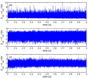
Figure 2.5: Isat signals for LHD plasma 44190: (a) tip 16; (b) tip 17; (c) tip 18.
to varying degrees; significant differences between the tips, separated by 6mm, can be seen. Fluctuations measured by tip 16 are dominated by positive intermittent bursts with large amplitudes; tip 17 is characterised by negative intermittent bursts with smaller amplitudes; and the time series for tip 18 is almost symmetric. Similar behaviour can be observed with a different set of three probes by altering the position of the plasma in LHD [Ohno et al., 2006b].
2.4.2 Scaling properties
We now examine the statistical properties of the LHD Isat signals. We use the power
1 2 3 4 0 2 4 6 8 10 log
10[τ (µs)]
log 10 [S m ( τ
)] Region I Region II
(a)
101 102 103 104 105 10−7 10−6 10−5 10−4 10−3 Frequency (Hz) PSD (arb) (b)
1 2 3 4
0 2 4 6 8 10 log
10[τ (µs)]
log 10 [S m ( τ
)] Region I Region II
(c)
101 102 103 104 105 10−7 10−6 10−5 10−4 10−3 Frequency (Hz) PSD (arb) (d)
1 2 3 4
0 2 4 6 8 10 log
10[τ (µs)]
log 10 [S m ( τ )] (e)
101 102 103 104 105 10−7 10−6 10−5 10−4 10−3 10−2 10−1 Frequency (Hz) PSD (arb) (f)
regions of scaling separated at about τ = 40µs for tip 16 and τ = 30µs for tip 17. Tip 18, however, shows only one region of scaling with scaling exponentα close to 1. In contrast with absolute moments, the PSDs do not exhibit a clear region of scaling, except for tip 17 which shows power-law scaling of the form ∼ f−β with β = 1.7 in the region 10-100kHz, corresponding to 10-100µs. A low frequency coherent mode at fcm ≃390Hz, together with higher harmonics, appears in all PSDs, and is marked by a dashed line in each PSD in figure 2.6. Its amplitude is smallest for tip 16 and largest for tip 18. The reciprocal of the frequency of this coherent mode,1/fcm, is also marked on each absolute moment plot by a dashed line.
The scaling behaviour of tip 18 is very close to that of the second test case, figure 2.2(a): absolute moments scale with scaling exponentαclose to1forτ less than1/fcm and a dip aroundτ = 1/fcm. It is clear the that signal from tip 18 is strongly affected by the presence of the coherent mode. Absolute moments for tip 17 are also affected but to a lesser degree; there is small flattening around τ = 1/fcm. There appears to be little or no effect on the absolute moments for tip 16; this might be expected as the amplitude of the coherent mode in the PSD is relatively low.
It is clear that the presence of a coherent mode in the signal affects its scaling properties. We have therefore filtered out the coherent modes and harmonics in each time series by applying Chebyshev type I bandstop filters to peaks in the PSD which rise above2.5×10−4 of our arbitrary units. This corresponds to filtering out a single mode
at frequencyfcm≃390Hz for tip 16, 2 modes atfcmand2fcmfor tip 17 and 4 modes atfcm,2fcm,3fcm and4fcmfor tip 18.
100 101 102 103 104 105 0 0.2 0.4 0.6 0.8 1
lag (µs)
Autocorrelation
(a)
100 101 102 103 104 105 0 0.2 0.4 0.6 0.8 1
lag (µs)
Autocorrelation
(b)
100 101 102 103 104 105 0 0.2 0.4 0.6 0.8 1
lag (µs)
Autocorrelation
(c)
100 101 102 103 104 105 0 0.2 0.4 0.6 0.8 1
lag (µs)
Autocorrelation
(d)
101 102 103 104 105 −0.4 −0.2 0 0.2 0.4 0.6 0.8 1
lag (µs)
Autocorrelation
(e)
100 101 102 103 104 105 0 0.2 0.4 0.6 0.8 1
lag (µs)
Autocorrelation
(f)
LHD 16 LHD 17 LHD 18 MAST Decorrelation time,τA 40µs 30µs 130µs 60µs
Sm break,τm 40µs 30µs 45µs 30µs
Half-width of conditional average peak,τC 13µs 12µs 15µs 13µs Skewness time scale,τS 220µs 110µs 10µs 500µs
Table 2.1: Measured time scales.
Practically, this is achieved by finding a first crossing of an arbitrary, but small, threshold which in our case we set to0.05. Figure 2.7 shows the behaviour of the ACF before and after the filtering has been applied. The ACF for tip 18 is particularly affected; before filtering large oscillations appear, after filtering the ACF closely resembles that of the other two tips. Tip 17 is also affected; oscillations in the ACF are reduced for large values ofτ. The decorrelation timesτAobtained from the filtered data are presented in table 2.1. We see thatτAis about4 times larger for tip 18 than for tips 16 and 17 due to the slow fall-off of the ACF to zero.
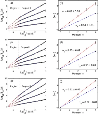
The results of absolute moments analysis of the filtered data are shown in figure 2.8. We note that, in principle, the complete characterisation of a dataset with N samples requires N moments. However, in practice one should only examine as many moments as can be safely computed from the finite size datasets that are studied. We find that the slow convergence of the higher moments prohibits us from computing moments higher than order four. Figures 2.8 (a), (c) and (e) show the first to fourth order absolute moments for fluctuations measured by tips 16, 17 and 18 respectively. All three tips now show two distinct regions of scaling, separated at about 40µs for tip 16, 30µs for tip 17 and 45µs for tip 18. We label this break in absolute moments τm and include it in table 2.1.
1 2 3 4 0 2 4 6 8 10 log
10[τ (µs)]
log 10 [S m ( τ
)] Region I Region II
(a)
0 1 2 3 4
0 1 2 3 Moment m ζ (m)
αI = 0.82 ± 0.09
αII = 0.51 ± 0.01 (b)
1 2 3 4
0 2 4 6 8 10 log
10[τ (µs)]
log 10 [S m ( τ
)] Region I Region II
(c)
0 1 2 3 4
0 1 2 3 Moment m ζ (m) (d)
αII = 0.55 ± 0.01 αI = 0.83 ± 0.07
1 2 3 4
0 2 4 6 8 10 log
10[τ (µs)]
log 10 [S m ( τ
)] Region I Region II
(e)
0 1 2 3 4
0 1 2 3 Moment m ζ (m)
αII = 0.67 ± 0.01 (f)
[image:57.595.141.488.175.576.2]αI = 0.91 ± 0.03
Figure 2.8: Absolute moments of order1≤m≤4(left) and derived scaling exponents ζ(m)(right) forIsatsignal of LHD plasma 44190 with bandstop filters applied to remove
reported in MAST with the scaling break at 40-60µs [Hnat et al., 2008; Dudson et al., 2005]. It is believed that scaling exponents uniquely characterise time series and, in cases such as Kolmogorov turbulence or critical systems, may offer the connection to phenomenological description. It is therefore of interest to compare the values of the scaling exponent α that are obtained in these two regimes for different confinement systems. The average value for the short time scale scaling parameterαI obtained from three similar MAST plasmas in [Hnat et al., 2008] is0.94±0.07, whereas the values of αI in LHD for tips 16 and 17 fall below this. However, tip 18 hasαI = 0.91±0.03; this value overlaps with that of the Hurst exponent for MAST L-mode plasma 6861, obtained for fluctuating time scales less than 30µs using three different algorithms in [Dudson et al., 2005]. In the longer time scale scaling region there are some notable similarities: MAST plasma 14218 hasαII = 0.59±0.04, overlapping withαII = 0.55±0.01 for tip 17 of LHD plasma 44190; MAST plasmas 14219 and 14220 haveαII = 0.64±0.02and αII = 0.65±0.02, overlapping withαII = 0.67±0.01 for tip 18 of LHD plasma 44190. These quantitative matches suggest a degree of universality in the properties of edge turbulence on times scales&40µs for the different plasmas examined. These results, as well as a larger comparative study of Carreras et al. [Carreras et al., 1998], suggest that exponents characterising long temporal correlations,αII, cluster in the region0.5−0.7.
2.5
MAST scaling
200 210 220 230 240 250 260 270
−2 0 2 4 6 8 10
time (ms)
(I sat
−<I
sat
>)/
σ
Here, we apply the absolute moment analysis to data taken from MAST L-mode plasma 14222 as a comparison to the LHD results. The data is taken from a reciprocating Langmuir probe located at the outboard midplane on MAST, and samples at a frequency of 500kHz. We prepare the data by removing linear trends, subtracting the mean and dividing by the standard deviation. Figure 2.9 shows the resulting data which is used in the analysis. The MAST data, like the LHD data, is bursty and intermittent and contains structures on many different time scales.
0 1 2 3
0 2 4 6 8 10 log
10[τ (µs)]
log
10
[S
m
]
Region I Region II
(a)
0 1 2 3 4
0 1 2 3 Moment m ζ (m) α
I = 0.89 ± 0.05
αII = 0.55 ± 0.05
(b)
Figure 2.10: (a) 1st to 4th order absolute moments for MAST 14222. Two scaling regions are evident with a break at 30µs. (b) Estimation of α for the two scaling regions.
100 102 104
0 0.2 0.4 0.6 0.8 1
Lag (µs)
Autocorrelation
(a)
101 102 103 104 105
10−3 10−4 10−5 10−6 10−7 Frequency (Hz) PSD (arb) (b)
Figure 2.11: (a) Autocorrelation function and (b) PSD for MAST plasma 14222.
![Figure 1.1: Cross sections for various fusion reactions [Wesson, 2004].](https://thumb-us.123doks.com/thumbv2/123dok_us/9707656.471890/19.595.221.418.104.245/figure-cross-sections-various-fusion-reactions-wesson.webp)
![Figure 1.9: The physics of the drift wave. Adapted from [Chen, 1984].](https://thumb-us.123doks.com/thumbv2/123dok_us/9707656.471890/38.595.235.409.432.639/figure-physics-drift-wave-adapted-chen.webp)
![Figure 2.3: (a) Location of the Langmuir probe array within LHD [Ohno et al., 2006b].(b) Location of probes within probe array [Ohno et al., 2006b].](https://thumb-us.123doks.com/thumbv2/123dok_us/9707656.471890/51.595.242.399.433.556/figure-location-langmuir-probe-array-ohno-location-probes.webp)