The stability of charged particle motion in sheared magnetic reversals

University of Warwick institutional repository: http://go.warwick.ac.uk/wrap

This paper is made available online in accordance with

publisher policies. Please scroll down to view the document

itself. Please refer to the repository record for this item and our

policy information available from the repository home page for

further information.

To see the final version of this paper please visit the publisher’s website.

Access to the published version may require a subscription.

Author(s): M. TSALAS, S. C. CHAPMAN and G. ROWLANDS

Article Title: The stability of charged-particle motion in sheared magnetic

reversals

Year of publication: 2001

Link to published version:

The stability of charged-particle motion in

sheared magnetic reversals

M. T S A L A S, S. C. C H A P M A N and G. R O W L A N D S

Department of Physics, University of Warwick, Coventry CV4 7AL, UK

(Received 20 November 2000)

Abstract.We consider the motion of charged particles in a static magnetic reversal with a shear component, which has application for the stability of current sheets, such as in the Earth’s geotail and in solar flares. We examine how the topology of the phase space changes as a function of the shear componentby. At zeroby, the phase space may be characterized by regions of stochastic and regular orbits (KAM surfaces). Numerically, we find that as we varyby, the position of the periodic orbit at the centre of the KAM surfaces changes. We use multiple-timescale perturbation theory to predict this variation analytically. We also find that for some values of

by, all the KAM surfaces are destroyed owing to a resonance effect between two timescales, making the phase space globally chaotic. By investigating the stability of the solutions in the vicinity of the fixed point, we are able to predict for what values ofby this happens and when the KAM surfaces reappear.

1. Introduction

Particles moving in the current sheet will, in a collisionless plasma, carry the current that supports it. Of relevance to the stability of current sheets under slow change is an understanding of single-particle dynamics in static field reversals. Simple models for such a field are magnetic reversals of the form

b= [f(z), by, bz], (1.1)

where f(z) is an odd function, usually taking the form either of the Harris field (Harris 1962), for whichf(z) = tanhz, or of the parabolic model, for whichf(z) =z. The parametersbyandbzare non-vanishing constants. Most of the analytical work in this paper gives the general treatment (anyf). However, in order to evaluate the final integrals and to make predictions, we revert for simplicity to the parabolic approximation. The two models converge inside the reversal, but diverge when |z|>1, with the parabolic model not allowing particles to escape. Since our results deal mainly with trajectories lying in the vicinity of the reversal, for which|z|<1, the region of validity of the parabolic model is sufficient. A convective electric field Ecan also be taken into account with a de Hoffman–Teller frame transformation (de Hoffman and Teller 1950). For convenience, we work in the frame of reference whereE= 0. A schematic diagram of the field lines in the coordinate system used is shown in Fig. 1.

3

2

1

0

–1

–2

–3

0 5 10 15 20 25 30 35

Parabolic Harris

x z

Figure 1.The coordinate system and the field lines used.

and references therein). For a comprehensive introduction to the subject, the reader is referred to the review paper by Chen (1992). The time-dependent system has, for theby = 0 case, also been studied elsewhere (Chapman 1994).

In the static case, it was found by Chen and Palmadesso (1986) and by Buchner and Zelenyi (1986) that for non-zerobz, the system is non-integrable, having only two global constants of the motion in involution, and that it can in general support three types of trajectory, namely regular (lying on KAM surfaces), chaotic and transient. Using Poincar´e surfaces of section, it was shown that each family of trajectories covers a distinct region in phase space, the geography of which varies as a function of the field parameters and of the energy.

However, since both the geotail and solar flares have been reported to possess a finite by field component (see e.g. Sergeev et al. 1993; Litvinenko 1996), it has become necessary to understand how the resulting shearing of the field lines affects the particle motion (see e.g. Karimabadi et al. 1990; Buchner and Zelenyi 1991; Zhu and Parks 1993). Recently, Chapman and Rowlands (1998) also investigated the finite-byproblem and obtained expressions for the bounce period and the action integral associated with the bouncing motion. They also showed that for certainby intervals, all the regular trajectories are destroyed, making the phase space globally chaotic. Ynnerman et al. (2000) demonstrated that the route to global chaos in the

by0 case is via repeated period doublings. In the same paper, it was shown that by deforms the tori on which the regular trajectories lie, squashing them into a M¨obius-strip-like shape.

For a charged particle moving in the magnetic field given by (1.1), the equations of motion can be obtained from the Lorenz force law. In a suitable normalization, they are

d2_φ

dτ2 =b2z[F(z)−φ]−bybzdz_dτ, (2.1) d2_z

dτ2 =

by bz

dφ

dτ −f(z)[F(z)−φ], , (2.2)

and the energy equation is ,

h= _b1₂ z

dφ dτ

2 +

dz dτ

2

+ [F(z)−φ]2_{, , (2.3)} where F(z) = R f(z)dz, φ = bzx−py (py is the y momentum, and the second invariant of the motion) and we have used they invariance of the field to reduce it to a two-dimensional problem. The full derivation of these equations and the normalization used can be found in Chapman and Rowlands (1998).

A convenient way to visualize the numerical solutions of these equations is the

z = 0 Poincar´e surface of section, which consists of injecting into the field a large number of particles, all with the same energyhandpy, but each with a different initial condition, such that all the phase space is explored. Every time the trajectory crosses thez= 0 plane it leaves a trace. It should be noted that while for theby = 0 case, the ˙z > 0 and the ˙z < 0 surfaces of section are identical, this is no longer the case when by 0. However, since both surfaces of section sample the same trajectories, it is sufficient to concentrate solely on one of the two. Here the ˙z >0 surface of section is used.

Examples of z = 0 surfaces of section for by = 0 can be found in Chen and Palmadesso (1986) and in Buchner and Zelenyi (1986). Their evolution as a function ofbyis shown in Buchner and Zelenyi (1991) and in Chapman and Rowlands (1998), where regions of global chaos are apparent for certain values ofby. The bifurcation sequence leading to the onset of global chaos can be found in Ynnerman et al. (2000), where it is also shown that the position of the central periodic orbit on the surface of section varies as a function ofby.

Here we shall use as examples three values ofh, namelyh= 0.001,h= 0.01 and

h= 0.1. We shall investigate the effect ofby both on single trajectories and on the phase-space topology.

3. The effects of

b

on single trajectories

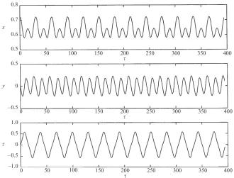
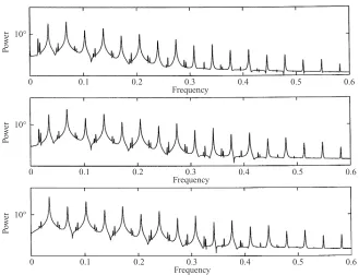
It is instructive to examine the effect ofby on single trajectories. Figures 2 and 3 show thex, yandzcomponents of two quasiperiodic trajectories in the vicinity of the central periodic orbit – the first forby = 0 and the second for by = 0.005. For both trajectoriesh= 0.01,py= 0 andbz= 0.1. In the corresponding power spectra (Figs 4 and 5), we see that whilst for the by = 0 case thexandz oscillations are distinct (exhibiting one fast oscillation and a slower modulation), when a finiteby is introduced they modulate each other, with the power spectra of each component of the motion exhibiting two modulations (corresponding to the originally separate

0.70

0.65

0.60

0.55

0 50 100 150 200 250 300 350 400

s

x

0.4

0.2

0

– 0.2

– 0.4

y

0 50 100 150 200 250 300 350 400

s

– 0.5

–1.0 0 0.5 1.0

z

0 50 100 150 200 250 300 350 400

s

Figure 2.Thex, yandzcoordinates of a quasiperiodic orbit initiated atx= 0.6849,z= 0,

vx= 0 forh= 0.01,py= 0,bz= 0.1 andby= 0.

0.8

0.7

0.6

0.5

0 50 100 150 200 250 300 350 400

s

x

0.5

0

– 0.5

y

0 50 100 150 200 250 300 350 400

s

– 0.5

–1.0 0 0.5 1.0

z

0 50 100 150 200 250 300 350 400

s

Figure 3.Thex, yandzcoordinates of a quasiperiodic orbit initiated atx= 0.72125,z= 0,

0 0.1 0.2 0.3 0.4 0.5 0.6 Frequency

10°

Powe

r

10°

Powe

r

10°

Powe

r

0 0.1 0.2 0.3 0.4 0.5 0.6

Frequency

0 0.1 0.2 0.3 0.4 0.5 0.6

Frequency

Figure 4.The power spectra of thex, yandzcomponents of the motion of the orbit shown in Fig. 2 (by= 0).

0 0.1 0.2 0.3 0.4 0.5 0.6

Frequency 10°

Powe

r

10°

Powe

r

10°

Powe

r

0 0.1 0.2 0.3 0.4 0.5 0.6

Frequency

0 0.1 0.2 0.3 0.4 0.5 0.6

Frequency

– 0.03 – 0.02 – 0.01 0 0.01 0.02 0.03

– 0.3 – 0.2 – 0.1 0 0.1 0.2 0.3

x

(a) by= 0.1

– 0.3 – 0.2 – 0.1 0 0.1 0.2 0.3

x

(b) by= 0.145

vx

– 0.03 – 0.02 – 0.01 0 0.01 0.02 0.03

vx

– 0.03 – 0.02 – 0.01 0 0.01 0.02 0.03

– 0.3 – 0.2 – 0.1 0 0.1 0.2 0.3

x

(c) by= 0.17

– 0.3 – 0.2 – 0.1 0 0.1 0.2 0.3

x

(d) by= 0.2

vx

– 0.03 – 0.02 – 0.01 0 0.01 0.02 0.03

vx

Figure 6.z= 0 surface-of-section plots forh= 0.001 and for increasingby. The other

parameters arebz= 0.1 andpy= 0.

4. The effect of

b

on the

z

= 0

surfaces of section

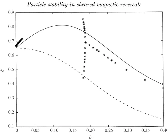
Forh= 0.001, the evolution of the phase space for increasingbyis shown in Fig. 6. At this energy, there is initially no quasi-integrable region (see Chen and Palmadesso 1986). However, asbyis increased, a quasi-integrable region appears via a pitchfork bifurcation at around by ≈ 0.145 (see Ynnerman et al. 2000). As by is further increased, the near-integrable region grows in size until it covers the whole of the surface of section (theby → ∞limit is integrable). In addition, thexposition of the central periodic orbit varies as a function of by. This variation is shown in Fig. 7, where the form of the bifurcation is shown, as determined numerically from the surfaces of section. Superimposed are the analytical results obtained in the next section.

0.30

0.25

0.20

0.15

0.10

0.05

0

0.10 0.15 0.20 0.25 0.30 0.35 0.40

by

xc

Figure 7.Comparison between the numerical (∗) and analytical (—– for ˙z >0; – – – for ˙z <0) results for the x(φ) position of the central periodic orbit onz = 0 as a function ofby for h= 0.001 andbz = 0.1.

120

100

80

60

40

20

0

0.08 0.10 0.12 0.14 0.16 0.18 0.20

by

T

140 160 180 200

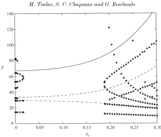
Figure 8.Comparison between numerical and analytical results for the observed periods in the vicinity of the central periodic orbit as a function ofbyforh= 0.001. The numerically

determined periods (fast and slow) are shown with a (∗). For the analytical results, the continuous line (—–) corresponds toTs, the dashed line (– – –) to 1₂Tsand the dashed–dotted

120

100

80

60

40

20

0

0 0.05 0.10 0.15 0.20 0.25 0.30

by

T

140

Figure 9.Comparison between the numerical (∗) and the analytical results for the observed periods in the vicinity of the central periodic orbit as a function of by forh = 0.01. The

numerically observed periods (fast and slow) are shown with a (∗). For the analytical re-sults, the continuous line (—–) corresponds toTs, the dashed line (– – –) to 1₂Ts and the

dashed–dotted line (–·–) to ¯Tf.

of trajectories in the vicinity of the central periodic orbit for each value ofby. At the specific value of by corresponding to where bifurcation occurs, the two slow frequencies become equal. Importantly, the value towards which they converge is equal to twice the fast period. Thus it appears that the reason the fixed point becomes unstable is that the higher-order harmonics of the slow periods overlap with the fast period. This coupling leads to the destruction of all the regular trajectories. One can also observe an additional periodicity in the motion that tends to infinity near the bifurcation and is a clear signature that the periodic trajectory becomes unstable. In addition, for values ofby where the slow period is smaller than twice the fast period, no regular trajectories exist.

A similar argument can be used forh= 0.01, the surfaces of section of which can be found in Chapman and Rowlands (1998) and Ynnerman et al. (2000). Here we show the evolution of the largest periods observed in Figs 4 and 5 as a function of

by (Fig. 9). In this case, a quasi-integrable region exists in the vicinity ofby = 0, but subsequently disappears via an inverse pitchfork bifurcation atby≈0.017, and reappears atby ≈0.178. In Fig. 10, we also show the position of the fixed point on z= 0 as a function ofby.

As a third example, we use h = 0.1, for which it is found (Fig. 11) that the timescales always remain well separated and that the quasi-integrable region always exists. The position of the fixed point onz = 0 as a function ofby for this energy level is shown in Fig. 12.

0.5

0.4

0.3

0.2

0.1

0 0.05 0.10 0.15 0.20 0.35 0.40

by

0.30 0.25 0.7

0.6 0.8

xc

Figure 10.Comparison between the numerical (∗) and the analytical (—– for ˙z >0; – – – for ˙

z <0) results for thex(φ) position of the central periodic orbit onz= 0 as a function ofby

forh= 0.01 andbz= 0.1.

120

100

80

60

40

20

0

0 0.05 0.10 0.15 0.20 0.25 0.30

by

T

140

0.35 0.40 0.45 0.50

Figure 11.Comparison between the numerical (∗) and the analytical results for the observed periods in the vicinity of the central periodic orbit as a function ofby for h = 0.1. The

numerically determined periods (fast and slow) are shown with a (∗). For the analytical results, the continuous line (—–) corresponds toTsand the dashed line (– – –) to ¯Tf.

5. The perturbation procedure

1.6

1.4

1.2

1.0

0.8

0 0.05 0.10 0.15 0.20 0.35 0.40

by

0.30 0.25 2.0

1.8 2.4

2.2

xc

0.45 0.50

Figure 12.Comparison between numerical (∗) and the analytical (—– for ˙z > 0; – – – for ˙

z <0) results for thex(φ) position of the central periodic orbit onz= 0 as a function ofby

forh= 0.1 andbz = 0.1.

essentially of taking the oscillatory solution obtained by applying conventional perturbation theory and making the phase slowly time-varying. The formal way of doing this is to separate the timescales between thezmotion, which is fast, and the

xmotion, which has a slower component. Thus one can think of a fast timescale (τf) in which a particle oscillates up and down in thezaxis, and a slow timescale (τs), in which the particle rotates around the KAM surface in the (x,x˙) plane. Then, using

bzas our expansion parameter (i.e. assuming thatbz1), we can writeτs=bzτf, and hence

d dτ =

d dτf +bz

d dτs.

Thus, by expandingzandφin the form (Chapman and Rowlands 1998)

φ=φ0(τs) +bzφ1(τf, τs) +b2zφ2(τf, τs) +. . . , (5.1a) z=z0(τf, τs) +bzz1(τf, τs) +b2zz2(τf, τs) +. . . , (5.1b) the equations of motion yield, to lowest order,

d2_φ 0

dτ2

f = 0, (5.2)

d2_z 0

dτ2 f =by

dφ0

dτs + dφ1

dτf

−f(z0)[F(z0)−φ0] (5.3)

and

h0≡h=

dz0

dτf

₂

+

dφ0

dτs + dφ1

dτf

₂

d2_φ1

dτ2 f =−by

dz0

dτf. (5.5)

And to orderb2 z, d2_φ 0

dτ2 s + 2

d2_φ 1

dτfdτs + d2_φ

2

dτ2 f

= [F(z0)−φ0]−by

dz0

dτs + dz1

dτf

. (5.6)

Chapman and Rowlands (1998) solved (5.2)–(5.6), by showing that the action inte-gralH(dz0/dτf)dz0 is, to lowest order, a constant of the motion. In this paper, we are primarily interested in the bifurcation process, so we can use linear perturbation theory about the Chapman and Rowlands solution. Thus we can write

φ0(τs) = ¯φ0+δφ0(τs), (5.7a) z0(τf, τs) = ¯z0(τf) +δz0(τf, τs), (5.7b) where ¯φ0 is now a strict constant during an oscillation, corresponding to the pos-ition of the central periodic orbit, and ¯z0(τf) corresponds toz0on ¯φ0. The small el-ementδφ0(τs) is the linearization about the central orbit. Expandingφ1, φ2, . . .and

z1, z2, . . .in the same way and substituting into (5.2)–(5.6) yields for ¯φ0, ¯φ1,φ¯2,z¯0 and ¯z1

d2_z¯ 0

dτ2 f =by

dφ¯1

dτf −f( ¯z0)[F( ¯z0)− ¯

φ0], (5.8)

¯

h0 ≡h0=

dz¯0

dτf

2 +

dφ¯1

dτf

2

+ [F( ¯z0)−φ¯0]2, (5.9)

d2_φ¯ 1

dτ2 f =−by

dz¯0

dτf (5.10)

and

d2_φ¯ 2

dτ2

f = [F( ¯z0)− ¯

φ0]−byd_dτz¯1

f. (5.11)

Similarly, forδφ0, δφ1, δφ2, δz0 andδz1, we obtain the equations

d2_δz 0

dτ2 f =by

dδφ0

dτs + dδφ1

dτf

− d

dz¯0{f( ¯z0)[F( ¯z0)− ¯

φ0]}δz0+f( ¯z0)δφ0 (5.12)

d2_δφ 1

dτ2 f

=−bydδz_dτ0

f (5.13)

and

d2_δφ 0

dτ2 s + 2

d2_δφ 1

dτfdτs+ d2_δφ

2

dτ2 f

= [f( ¯z0)δz0−δφ0]−by

dδz0

dτs + dδz1

dτf

. (5.14)

6. The position of the central periodic orbit

We first consider the solution to lowest order that corresponds to a periodic orbit passing through the ¯z0= 0 plane on ¯φ0. Equation (5.10) can be integrated once to give

dφ¯1

dτf =−byz¯0+ ¯K, (6.1)

where ¯K is the constant of integration. Since we are looking for the periodic sol-utions of ¯z0 (period ¯Tf), we demand that ¯φ1 is also periodic with the same fast period; that is, ¯φ1(τf) = ¯φ1(τf+ ¯Tf). By integrating (6.1) over a period, we obtain for ¯K

¯

K= b_¯y

Tf

Z _T¯_f

0 z¯0dτf. (6.2)

It follows that if ¯z0 is symmetric over a period then ¯K = 0. This symmetry can be observed in the numerical integration of the full equations (Figs 2 and 3), and is a feature only of the central periodic orbit, that is of ¯z0(τf), and not of any near-integrable orbitz0(τf, τs). By substituting fordφ¯1/dτf into (5.9), we obtain

dτf =±q dz¯0 ¯

h0−b2yz¯02−[F( ¯z0)−φ¯0]2

, (6.3)

and the fast period will be twice the time the particle needs to go from one extreme to the other:

¯

Tf= 2

Z _z¯c

−z¯0

dz¯0

q

¯

h0−b2yz¯02−[F( ¯z0)−φ¯0]2

, (6.4)

where ¯zc is the positive root of the denominator, that is, wheredz¯0/dτf = 0. The positive root of (6.3) is used, since the integration is in the positivedz¯0/dτf direc-tion. To evaluate this integral, we choose the parabolic approximation, for which

f( ¯z0) = ¯z0. Then

¯

zc=

q

2(√D+ ¯φ0−b2y), (6.5)

where

D= ( ¯φ0−b2y)2+ ¯h0−φ¯20, (6.6) and the integral in (6.4) can be evaluated to yield

¯

Tf = 8¯gK(¯k), (6.7)

where, as before,K(¯k) is the complete elliptic integral of the first kind,

¯

k=

s

1 2+

¯

φ0−b2y

2√D (6.8)

and

¯

g=

s

1

4√D (6.9)

In the same way, by integrating (6.3) fromτftoτfc(corresponding to ¯zc), we obtain τfc−τf = 2¯gF

¯

z0= ¯zccn τf−_2¯gτfc,k¯ , (6.11) whereτfc can be obtained by setting an initial condition forz. Choosing ¯z0= 0 on

τf = 0 yields

τfc = 2¯gK(¯k). (6.12)

Note that the solution of ¯z0 is symmetric in time, which is consistent with taking ¯

K= 0.

Now, in order to obtain an expression for the position of the central periodic orbit as a function of by, it is noted that (5.11) can be integrated over a period, and by insisting that ¯φ2and ¯z1are periodic with period ¯Tf, we obtain the following equation for ¯φ0:

¯

φ0= _T2_¯ f

Z _z¯c

−z¯c

F( ¯z0)dz¯0

q

¯

h0−b2yz¯02−[F( ¯z0)−φ¯0]2

. (6.13)

Again, forf( ¯z0) = ¯z0, the integral can be evaluated, and we find ¯

φ0= 2 √

D

E(k)

K(k)− 1 2

+ ( ¯φ0−b2y). (6.14)

Unfortunately, it is not possible to solve this equation analytically for ¯φ0. By solving it numerically for the same three values of ¯h0used in the numerical simulations and as a function ofby, we obtain the dashed lines in Figs 7, 10 and 12.

Since we have demanded that ¯φ0be a strict constant, the difference between the position of the particle as it crosses the z = 0 plane going up and going down is not apparent. Therefore, in order to obtain a better approximation for the position of the central orbit and to show the asymmetry between the ˙z >0 and the ˙z <0 diagrams, it is necessary to go to higher order, that is to look at ¯φ1. By integrating (6.1) overτf (for ¯K= 0), we obtain for ¯φ1the expression

¯

φ1=−by

Z _τf

¯

z0dτf+ ¯C, (6.15)

where ¯Cis the constant of integration. The integral can be evaluated forf( ¯z0) = ¯z0, to yield

¯

φ1 =−2byarccos

"s

1−k2_sn2

τf−τfc 2¯g ,k¯

#

+ ¯C. (6.16)

To obtain a value for the constant ¯C, we observe from the form of the expected trajectory (Fig. 13) that ¯φ1(τf = 1₄T¯f) = 0, which yields ¯C= 0. After some simpli-fications, we obtain for the value of ¯φ1on ¯z0= 0

¯

φ1|z¯0=0=−byarccos − ¯

φ0_√−b2y D

!

. (6.17)

The continuous lines in Figs 7, 10 and 12 then correspond to ¯φ0+bzφ¯1|z¯0=0. We see that they are in relatively good agreement (to orderb2

agree-z

zc

φ0 φ1 φ1

φ

Figure 13.The path of integration used to calculate ¯φ1|z¯0=0.

ment between numerical and analytical results is best far from the bifurcations, since perturbation theory is no longer valid in their vicinity.

7. The stability of the central periodic orbit

To investigate the stability of the central periodic orbit, we must look at the slow variationδφ0(τs). To do this, we integrate (5.6) over a fast periodTf(τs), insist-ing that φ1(τf, τs), φ2(τf, τs) andz1(τf, τs) be periodic in the fast period; that is, φ1(τf, τs) =φ1(τf+Tf(τs), τs), etc. We obtain the equation

d2_φ0

dτ2 s =

1

Tf(τs)

Z Tf(τs)

0 dτf

F(z0)−φ0−bydz_dτ0 s

, (7.1)

and by linearizing as before, using (5.7), we obtain for ¯φ0 equation (5.11), and for

δφ0the expression

d2_δφ 0

dτ2

s +δφ0 = 1 ¯

Tf

Z T¯f

0 dτf

f( ¯z0)δz0−bydδz_dτ0 s

−φ¯0δT_T¯f

f , (7.2)

where

Tf(τs) = ¯Tf+δTf(τs). (7.3) In order to evaluate the integral on the right-hand side, an expression forδz0is required. To obtain it, we begin by integrating (5.13) once. This gives

dδφ1

dτf =−byδz0+δK(τs), (7.4)

whereδK(τs) is an integration constant given by

δK(τs) =byhδz0i (7.5)

where from now on the notation used is

h. . .i= 1_¯

Tf

Z _T¯_f

Lδz0 =by

dδφ0

dτs +δK

+f( ¯z0)δφ0, (7.6)

where the operatorLis defined as

L= d2

dτ2 f +b

2 y+_dd_z¯

0{f( ¯z0)[F( ¯z0)− ¯

φ0]}. (7.7)

Thus we can write

δz0 =byA(τf)

dδφ0

dτs +δK

+B(τf)δφ0, (7.8)

whereA and B are fast-varying functions, independent of the slow timescale. To obtain them, we must solve the following second-order differential equations:

LA= 1, (7.9)

LB=f( ¯z0). (7.10)

Integrating (7.8) over a fast period yields

hδz0i=byhAi

dδφ0

dτs +δK

+hBiδφ0, (7.11)

and by combining this with (7.5) and rearranging forδK(τs), we obtain

δK(τs) =

_b2

yhAi 1−b2

yhAi

dδφ0

dτs +

byhBi 1−b2

yhAi

δφ0, (7.12)

Finally, by substituting forδK(τs) into (7.8), we obtain forδz0 the expression

δz0=by

A+₁b₋2yA_bh₂Ai yhAi

dδφ0

dτs +

B+₁b₋2yA_bh₂Bi yhAi

δφ0. (7.13)

By substituting forδz0 into (7.2) and using (7.9) and (7.10), we can write (7.2) in the form

d2_δφ0

dτ2 s

1 1−b2

yhAi

+δφ0

1− hf( ¯z0)Bi −₁b₋2yh_bB₂i2 yhAi

=−φ¯0δT_T¯f

f . (7.14)

The details of how this form is obtained are given in Appendix A. To proceed, an expression for δTf(τs) is required. A method to obtain it is given in Appendix B. We find

δTf(τs) = 2_DK₅(¯_/k₄)

b2 y+

¯

φ0(¯h0−b2yφ¯0) ¯

h0−φ¯20

δφ0. (7.15)

In addition, the integrals hAi, hBiand hf( ¯z0)Bi need to be evaluated. This is done in Appendix C, where we find for the parabolic approximation

hAi= b_D2y, (7.16)

hBi= 0 (7.17)

and

hf( ¯z0)Bi= ¯

h0

By substituting these into (7.14), we obtain, after some simplifications,

d2_δφ 0

dτ2 s +ω

2

sδφ0= 0. (7.19)

Thus, to lowest order, the variation ofδφ0is simple-harmonic, with frequency

ω2 s=

¯

h0−2 ¯φ0b2y 2D

"_¯

h0−2 ¯φ0b2y ¯

h0−φ¯0b2y + ¯

φ0(¯h0φ¯0−2 ¯φ20b2y+ ¯h0b2y) (¯h0−φ¯20)D

#

. (7.20)

The slow period is then given by

Ts= _b2π

zωs. (7.21)

The analytically obtained periods and their harmonics are shown in Figs 8–11, superimposed on the numerical data. In all three cases, the analytical expression for Ts is qualitatively accurate, but it predicts higher values than expected from the numerical results. Also, the analytical predictions are more accurate for higher energies.

There is a good explanation for these discrepancies. One should keep in mind the fact that we had to linearize, a procedure that, as we saw in theby= 0 case, is not very accurate in the vicinity of a bifurcation. Buchner and Zelenyi (1986) showed for by = 0 that the value obtained for the slow period corresponds to the value towards which the actual solution converges for largeh. The fact that the accuracy of our results increases with increasing hsuggests that this is still true when aby component is introduced. However, the growing discrepancy between analytical and numerical values ofTsfor increasingby suggests that the convergence rate is slower for large values of by. In contrast, the prediction for ¯Tf is reasonable, with the accuracy again increasing for increasingh.

Numerically, we found that the destruction of the near-integrable region via a bifurcation occurs when the two slow periods (one of which we have obtained here, the other one being of higher order, corresponding to the slow periods ofz1andφ2) become equal to twice the fast period, leading to a resonance between the fast period and a higher-order harmonic of the slow period. In Fig. 8, we see that ¯Tf ≈1₂Tsat by≈0.1108, and this is therefore where we should expect the bifurcation to occur. The actual value where it occurs isby ≈0.145. The difference is mainly due to our large error in the calculation ofTs.

For the h= 0.01 case, we see that our approximation does not allow us to find the bifurcation, since, contrary to what is observed numerically, we find 1

2Tsto be always greater thanTf. Again, this is due to our high estimate ofTs. The sudden decrease inTsobserved numerically at by ≈0.01 is probably due to higher-order effects that are not included in the lowest-order approximation.

Finally, in Fig. 11, we observe that for h = 0.1, the prediction forTs is more accurate than in the previous two cases and that all the timescales remain well separated.

8. Conclusions

have also shown that asby increases, thexposition of the central periodic orbit in the Poincar´e surface of section varies. This variation has been obtained here ana-lytically by using a multiple-timescale perturbation technique around thebz = 0 solution. By linearizing around this fixed point, we have also provided analytical estimates (in some cases) for the value ofbyat which quasiperiodic orbits reappear via a bifurcation. These estimates correctly quantify the resonance effect leading to the onset of global chaos.

Appendix A. Derivation of (7.14)

By inserting (7.13) into (7.2) and using (7.9) and (7.10), we obtain the following coefficients for each term on the right-hand side of (7.2):

(a) ford2_δφ

0/dτs2, the coefficient is

*

−by byA+ b 3 yAhAi 1−b2

yhAi

!+

, (A 1)

which simplifies to

−₁₋b2y_bhA₂ i

yhAi; (A 2)

(b) fordδφ0/dτs, it is

*

LB byA+ b 3 yAhAi 1−b2

yhAi

!

−by B+ b 2 yAhBi 1−b2

yhAi

!+

, (A 3)

which is equal to zero, sincehLBAi=hLABi=hBi; (c) finally, the coefficient forδφ0 is

*

LB B+₁b₋2yA_bh₂Bi yhAi

!+

, (A 4)

which simplifies to

hf( ¯z0)Bi+₁b₋2yh_bB₂i2

yhAi. (A 5)

By putting all these terms together in (7.2), we obtain

d2_δφ0

dτ2

s +δφ0 = − b2

yhAi 1−b2

yhAi

!

d2_δφ0

dτ2

s + hf( ¯z0)Bi+ b2

yhBi2 1−b2

yhAi

!

δφ0−φ¯0δT_T¯f f ,

(A 6) which, after some simplifications, yields (7.14).

Appendix B. Obtaining an expression for

δT

By integrating (5.5) once and substituting the expression obtained fordφ1/dτfinto (5.4), we obtain, after some manipulations,

dτf = p dz0

where K(τs) is the integration constant obtained from the integration of (5.5). From our linearization, we know that K(τs) ≈ δK(τs) (since ¯K = 0) and that dφ0/dτs≈dδφ0/dτs. By substituting for these, we write

dτf = p dz0

h0−(byz0−)2−[F(z0)−φ0]2, (B 2) where the notation

= dδφ_dτ0

s +δK(τs) = 1 1−b2

yhAi dδφ0

dτs

has been used. We shall assume that is small and can be used as an expansion parameter. For the parabolic approximation, (B 2) can be further simplified by writing it in the form

dτf = 2p dz0 (a2_−z2

0)(b2+z02) + 8byz0, (B 3) where

a2 _{= 2}√_(φ

0−b2y)2+h0−φ20−2+φ0−b2y

(B 4) and

b2_{= 2}√_(φ

0−b2y)2+h0−φ20−2−φ0+b2y

. (B 5)

By expanding the denominator of (B 3) for small, we obtain

dτf = 2p dz0

(a−z0−γ)(a+z0+γ)(z20−2γz0+b2)+O(

2_{), (B 6)}

where

γ=− 4by

a2_+b2. (B 7)

The two roots of the denominator, corresponding to the turning points of z0, are −a−γanda−γ. Note that in this more general case,z0 is no longer symmetric. The fast periodTf(τs) is obtained by integrating twice from one turning point to the other:

Tf(τs) = 4

Z _a−γ

−a−γ

dz0

p

(a−z0−γ)(a+z0+γ)(z20−2γz0+b2)+O(

2_{). (B 8)}

By writingy=z0+γand expanding the non-singular term in the denominator of (B 8), we obtain

Tf(τs) = 4

Z _a

−a

dy

p

(a2_−y2_)(b2_+y2₎

1 +_b22₊γy_y2+O(2_{). (B 9)}

This integral can be evaluated to give

Tf(τs) = 8gK(k) +O(2), (B 10) where

k(τs) = √ a

a2_+b2 (B 11)

and

g(τs) = √ 1

¯

g+δg(τs), we obtain forδk(τs) andδg(τs)

δk(τs) = ¯

h0−b2yφ¯0

4¯kD3/2 δφ0 (B 13)

and

δg(τs) = b 2 y

4D5/4δφ0, (B 14)

andδTf(τs) is given by

δTf(τs) = 8K(¯k)δg+ 8¯gdK_dk¯(¯k)δk, (B 15) which, after some simplifications (and using (6.14)), becomes

δTf(τs) = 2_DK₅(¯_/k₄)

"

b2 y+

¯

φ0(¯h0−b2yφ¯0) ¯

h0−φ¯20

#

δφ0. (B 16)

Appendix C. Evaluating the integrals

h

A

i

,

h

B

i

and

h

f

( ¯

z

)

B

i

Ld_dτz¯0

f = 0. (C 1)

By writing

A= ˜Ad_dτz¯0

f (C 2)

and substituting into (7.9), we obtain, after some simplifications (for f( ¯z0) = ¯z0), the expression

dz¯0

dτf

−1 _d

dτf

"

dA˜ dτf

dz¯0

dτf

2#

= 1, (C 3)

which yields, after integration,

dA˜ dτf

dz¯0

dτf

2

= ¯z0+C1, (C 4)

or

dA˜ dτf =

¯

z0+C1

(dz¯0/dτf)2, (C 5)

where C1 is the constant of integration. By integrating over a fast period and insisting that ˜Ais periodic with period ¯Tf, we obtain thatC1= 0, since the integral

Z T¯f

0

¯

z0

(dz¯0/dτf)2dτf = 0. (C 6)

We know ¯z0 from (6.11), and therefore

dz¯0

dτf =− ¯

zc

where

s= _2¯τf_g −K(¯k). (C 8)

By integrating (C 5) from 0 to an arbitrary timeτf <2¯gK(¯k) (in order to avoid the singularity that exists atτf = 2¯gK(¯k)), we obtain

˜

A(τf)−A˜(0) =

Z _τf

0

¯

z0

(dz¯0/dτf)2dτf, (C 9) and by substituting into this the expressions for ¯z0 and dz¯0/dτf, we obtain, after some simplifications,

˜

A(τf)−A˜(0) = 8¯g 3 ¯

zc

Z _s

−K( ¯k)

cn(s,k¯)

dn2(s,k¯) sn2_(s,k¯₎ds. (C 10) The integral on the right-hand side of (C 10) can be evaluated, and we find for ˜

A(τf)

˜

A(τf) = 8¯g 3 ¯

zc ¯

k2_sn2_(s,k¯_)−dn2_(s,k¯)

sn(s,k¯) dn(s,k¯) +G+ ˜A(0), (C 11) where

G= 8¯_z¯g3 c

2¯k2₋₁ √

1−k¯2, (C 12)

and so

A(τf) =−4¯g2[¯k2sn2(s,k¯)−dn2(s,k¯)] + PF(τf), (C 13) where PF is a periodic function with period ¯Tfthat vanishes when integrated over a period. Note that in this expression, the singularities at τf = 2¯g(2n+ 1)K(¯k) (n integer) have disappeared andτf can proceed to 8¯gK(¯k) (that is, to cover a whole period). Finally,

hAi= _T1_¯ f

Z T¯f

0 A dτf=− ¯

g2

K(¯k)

Z _{3K( ¯k)}

−K( ¯k)[¯k

2_sn2_(s,k¯)−dn2_{(s,k¯)]ds (C 14)}

and, by evaluating the integral, we obtain

hAi= 8¯g2E(¯k)

K(¯k)− 1 2

. (C 15)

By using (6.14), the above expression can be simplified to the form

hAi= b_D2y. (C 16)

A similar argument can be used to findhBiandhf( ¯z0)Bi. By writing

B = ˜Bd_dτz¯0

f (C 17)

and substituting into (7.10), we obtain in the same way as before the relationship

dB˜ dτf =

1 2z¯02+C2

(dz¯0/dτf)2, (C 18)

C2=−1₂

R_T¯_f

0 z¯02(dz¯0/dτf)−2dτf

R_T¯_f

0 (dz¯0/dτf)−2dτf

(C 19)

Forf( ¯z0) = ¯z0, the integrals can be evaluated to give the following equation forC2:

C2=−z¯ 2 c 2

(1−k¯2_{)[2E(¯k)−K(¯k)]}

(2¯k2_{−1)E(¯k) + (1−k}¯2_)K(¯k), (C 20) and, in the same way as before, we find forhBiandhf( ¯z0)Bi

hBi= 0 (C 21)

and

hf( ¯z0)Bi= (1− ¯

k2_{)[1−2E(¯k)/K(¯k)] +E(¯k)}2_/K(¯k)2

(2¯k2_{−1)E(¯k)/K(¯k) + (1−k}¯2₎ ; (C 22) again, by using (6.14), this can be simplified to yield

hf( ¯z0)Bi= ¯

h0

2(¯h0−φ¯0b2y). (C 23)

References

Buchner, J. and Zelenyi, L. M. 1986 Deterministic chaos in the dynamics of charged particles near a magnetic field reversal.Phys. Lett.118A, 395.

Buchner, J. and Zelenyi, L. M. 1991 Regular and chaotic particle motion in sheared magnetic field reversals.Adv. Space Res.11, 9177.

Chapman, S. C. 1994 Properties of single particle dynamics in a parabolic magnetic reversal with general time dependence.J. Geophys. Res.99, 5977.

Chapman, S. C. and Rowlands, G. 1998 Are particles detrapped by constant By in static

magnetic reversals?J. Geophys. Res.103, 4597.

Chen, J. 1992 Nonlinear dynamics of charged particles in the magnetotail.J. Geophys. Res.

97, 15011.

Chen, J. and Palmadesso, P. J. 1986 Chaos and nonlinear dynamics of single-particle orbits in a magnetotaillike magnetic field.J. Geophys. Res.91, 1499.

de Hoffman, F. and Teller, E. 1950 Magnetohydrodynamic shock.Phys. Rev.80, 692. Harris, E. G. 1962 On a plasma sheath separating regions of oppositely directed magnetic

field.Nuovo Cim.23, 115.

Karimabadi, H., Pritchett, P. L. and Coroniti, F. V. 1990 Particle orbits on two-dimensional equilibrium models for the magnetotail.J. Geophys. Res.95, 17153.

Litvinenko, Y. E. 1996 Particle acceleration in reconnecting current sheets with a nonzero magnetic field.Astrophys. J.462, 997.

Rowlands, G. 1990Non-Linear Phenomena in Science and Engineering. Ellis Horwood, Chich-ester.

Sergeev, V. A., Mitchell, D. G., Russell, C. T. and Williams, D. J. 1993 Structure of the tail plasma/current sheet at∼11reand its changes in the course of a substorm.J. Geophys. Res.98, 17345.

Sonnerup, B. U. ¨O. 1971 Adiabatic particle orbits in a magnetic null sheet.J. Geophys. Res.

76, 2811.

Speiser, T. W. 1978 Particle trajectories in model current sheets, 1. Analytical solutions.

J. Geophys. Res.21, 627.

Ynnerman, A., Chapman, S. C., Tsalas, M. and Rowlands, G. 2000 Identification of symmetry breaking and a bifurcation sequence to chaos in single particle dynamics in magnetic reversals.PhysicaD139, 217.

Zhu, Z. and Parks, G. 1993 Particle orbits in model current sheets with a nonzeroBy