The water footprint related to reservoir operation on a global scale

(1)

1 Prof. dr. ir. A.Y. Hoekstra

MASTER THESIS

THE WATER FOOTPRINT RELATED

TO RESERVOIR OPERATION ON A

GLOBAL SCALE

L. Knook

FACULTY OF ENGINEERING TECHNOLOGY

DEPARTMENT OF WATER ENGINEERING AND MANAGEMENT

EXAMINATION COMMITTEE

ir. H.J. Hogeboom

(2)

(3)

3

The water footprint related to reservoir operation on a

global scale

Master thesis in Civil Engineering and Management

Faculty of Engineering and Technology

Department of Water Engineering and Management

University of Twente

August 2016

Version 1.0

Author: ing. L. Knook

Student number: 1490753

Email: l.knook-1@student.utwente.nl

lknook@hotmail.com

Phone: 0627128458

Graduation Committee:

Graduation supervisor: Prof. dr. ir. A.Y. Hoekstra

University of Twente

Daily supervisor: ir. H.J. Hogeboom

(4)

(5)

5

I. List of symbols

A Reservoir area ha

Ea Annual actual evaporation volume m3y-1

Ed Daily evaporation rate mmd-1

Ep The amount of evaporation from a Class A pan mmd-1

Ey Annual evaporation rate mmy-1

ETc Daily evaporation rate of the vegetation before there was a reservoir mmd-1

ETo Daily evapotranspiration rate mmd-1

Ev Annual evaporation volume m3y-1

Gsc The solar constant MJm-2min-1

J The number of the day between 1 January and 31 December (-)

N The maximal number of daylight hours h

P Production per reservoir purpose

Pr Annual precipitation volume mmy-1

Ra The extra-terrestrial radiation MJm-2d-1

Rn Net radiation expressed as mm evaporation mmd-1

Rs The incoming solar radiation MJm-2d-1

SVD The saturation vapour density gm-3

Ta The air temperature °C or °K

Td The dew point temperature °C or °K

U10 The average wind speed at a height of 10 m kmd-1

as The regression constant, expressing the fraction of extra-terrestrial radiation

reaching the earth on overcast days (n = 0)

(-) as+bs The fraction of extra-terrestrial radiation reaching the earth on clear days (-)

dr The inverse relative distance Earth-Sun (-)

ea The atmospheric vapour pressure kPa

es The saturation vapour pressure kPa

ew The saturated vapour pressure at air temperature kPa

kc The crop coefficient (-)

n The actual duration of sunshine in hours h

vi Annual economic value per purpose $y-1

vt Annual total economic value per reservoir $y-1

y The psychrometric constant kPa°C-1

Δ The slope of the saturated vapour pressure-temperature curve kPa°C-1

δ The solar decimation rad

κ Factor used to correct the maximal reservoir area (-)

ηi The allocation coefficient (-)

φ The latitude rad

(6)

(7)

7

II. Preface

With this thesis, I finalize my study Civil Engineering and Engineering at the University of Twente. I started with this master about 2 years ago, after I completed a bachelor Civil Engineering at the Hogeschool Utrecht and my premaster courses. This study started with a preparatory phase from September to November 2015, in which a literature review and research proposal were written and data was collected. The graduation project itself was conducted between December 2015 and July 2016. I expected beforehand that collecting the economic data, to determine the economic value of reservoirs, would be the most difficult part. But afterwards, it appeared that determining the evaporation from reservoir would be far more complex. Especially because it was difficult to extract climatological data for all the locations and the evaporation methods were not working well.

I would like to thank my supervisors from the University of Twente: Arjen and Rick. Arjen, thank you for the feedback and the suggestions on how to present my results. Rick, thank you for your advice during the whole project, your detailed feedback and your help with programming in Python. Also I would like to thank Mesfin, for his supervision during the preparatory course and the first month of my research. I also would like to thank my housemates in both Huize Ypelobrink and Huize Opdakken, for the “gezelligheid“ and for broadening my view on the world, in the time that I lived in both houses. I would like to thank my roommates in graduation room Z140, for their help with programming and for our talks about thesis problems. In the past year I have been in the board of S.K.V. Vakgericht and I would like to thank my fellow board members for not giving me too much “actiepuntjes”. Finally, I would like to thank Marit, for her love, support and for reviewing my thesis.

Luuk Knook

(8)

(9)

9

III. Summary

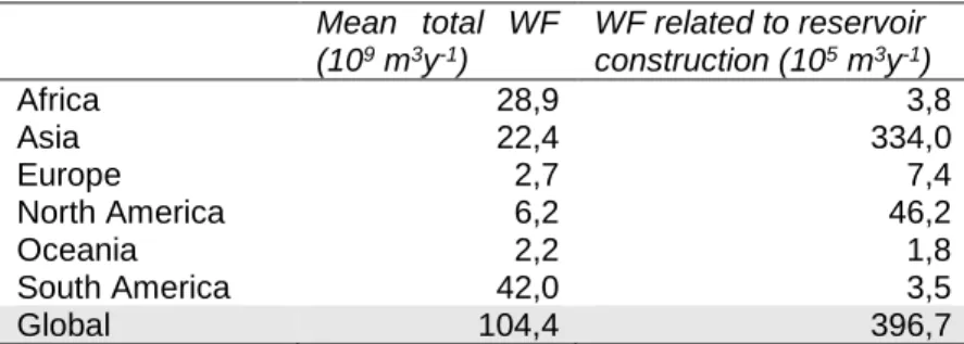
Reservoirs are used to generate electricity, supply water to irrigation, drinking water companies and the industry, to manage the water level in rivers to prevent flooding, to recreate and to catch fish. The water stored in reservoirs will be partly lost due to evaporation and this means that products and services produced by reservoirs have a water footprint. The objective of this study is to determine the water footprint related to the production of goods and services produced by man-made reservoirs.

Based on the WRD and the GRanD reservoir databases, a reservoir database is created with 2235 reservoirs. This corresponds to 3,8% of the reservoirs and 30,1 % of the total reservoir volume in the ICOLD database. The economic value of reservoirs is determined by multiplying the annual average production per purpose with the economic value per unit of production. No production data was available for the purpose residential and industrial water supply and therefore this was estimated based on the reservoir volume.

The evaporation was determined on a daily basis using 4 different methods: Jensen and Haise, Hamon, Penman and a method provided by Kohli and Frenken. With the first 3 methods, the evaporation was estimated based on climatological data provided by the ERA Interim database. Using the method of Kohli and Frenken, the evaporation is determined based on data from the FAO global evapotranspiration map and assuming that the crop coefficient for open water is 1. The evaporation volume is determined by taking the average of the 4 evaporation figures and multiply this, with the reservoir area and a factor to correct the reservoir area for the reservoir fullness.

The total water footprint per reservoir is the sum of both the water footprint related to evaporation and the water footprint related to reservoir construction. The water footprint of reservoir construction was based on the water footprint of construction materials and the dam body volume of the dam. Allocation coefficients based on the economic value of the reservoirs are used to allocate the water footprint to each reservoir purpose.

There can be concluded that all reservoir purposes treated in this study have a water footprint. The total annual water footprint from the reservoirs in this study is 1,04 x 1011_m3_{and the total annual economic}

value of the reservoirs purposes in this study is $ 311 billion, in 2014 U.S. Dollars. The total annual water footprint related to reservoir construction is 3,96 x 107_m3_{. The global water footprint related to:}

hydropower generation by reservoirs is 7,18 x 1010_m3_y-1_{, for irrigation water supply by reservoirs is 8,28}

x 109_m3_y-1_{, for flood prevention by reservoirs is 8,7 x 10}9_m3_y-1_{, for open water recreation on reservoirs}

is 2,01 x 109_m3_y-1_{, for residential and industrial water supply by reservoirs is 1,32 x 10}10_m3_y-1_{and for}

commercial fishing on reservoirs is 2,08 x 108_m3_y-1_.

(10)

(11)

11

IV. Samenvatting

Stuwmeren worden gebruikt om elektriciteit op te wekken, om water op te slaan ten behoeve van irrigatie, drinkwaterbedrijven of industrie, om waterstanden in rivieren te beïnvloeden en zo overstromingen te voorkomen, om te recreëren en om vis te vangen. Het water dat in stuwmeren is opgeslagen gaat echter deels verloren door verdamping. Dit betekent dat producten en diensten die geleverd worden door stuwmeren een watervoetafdruk hebben. Het doel van deze studie is om de watervoetafdruk, van de door stuwmeren geproduceerde producten en diensten, in kaart te brengen. Een database, bestaande uit 2235 reservoirs is samengesteld gebaseerd op gegevens uit de WRD en GRanD stuwmeren databases. Dit komt overeen met 3,8% van het totale aantal stuwmeren in de WRD-database en 30,1% van het totale stuwmeer volume in de WRD-WRD-database. De economische waarde van deze stuwmeren is bepaald door de productie per reservoir functie te vermenigvuldigen met de monetaire waarde per productie-eenheid. Er was geen productie informatie beschikbaar voor de functie drink- en industriewater onttrekking uit stuwmeren. Daarom is het onttrokken volume ingeschat op basis van het stuwmeer volume.

De verdamping uit stuwmeren is bepaald op basis van 4 verschillende methodes: Jensen and Haise, Hamon, Penman en de methode van Kolhi en Frenken. Met de eerste 3 methoden is de verdamping bepaald op basis van klimatologische gegevens uit de ERA Intrim database. De gebruikte methode van Kolhi en Frenken komt neer op het uitlezen van een FAO evapotranspiratie kaart voor elke reservoir locatie, met de aanname dat de gewas coëfficiënt voor open water 1 is. Het verdamping volume per stuwmeer is bepaald als het gemiddelde van de 4 verdampingsmethoden vermenigvuldigd met het oppervlak van het stuwmeer en een factor om het maximale stuwmeer oppervlak te corrigeren naar een jaarlijks gemiddelde oppervlak.

De totale watervoetafdruk per stuwmeer is de som van de watervoetafdruk gerelateerd aan verdamping en de watervoetafdruk gerelateerd aan het bouwen van het stuwmeer. De watervoetafdruk van het construeren van het reservoir is gebaseerd op de watervoetafdruk van bouwmaterialen en het volume van de stuwdam. Coëfficiënten op basis van de economische waarde zijn gebruikt om de watervoetafdruk toe te schrijven aan elke functie van het stuwmeer.

Er kan worden geconcludeerd dat alle functies van reservoirs, behandeld in deze studie, een watervoetafdruk hebben. De jaarlijkse watervoetafdruk van alle reservoirs in deze studie is 1,04 x 1011

m3 _{en de totale economische waarde van de stuwmeren in deze studie is $ 311 miljard, in 2014 U.S.}

Dollars. De totale jaarlijkse watervoetafdruk gerelateerd aan het bouwen van stuwmeren is 3,96 x 107

m3_{. De wereldwijde watervoetafdruk gerelateerd aan: het opwekken van elektriciteit door stuwmeren is}

7,18 x 1010_m3_j-1_{, het opslaan van water ten behoeve van irrigatie is 8,28 x 10}9_m3_j-1_{, voor het voorkomen}

van overstromingen door stuwmeren is 8,7 x 109_m3_j-1_{, ten behoeve van het recreëren op stuwmeren is}

2,01 x 109_m3_j-1_{, het opslaan van water ten behoeve van de drinkwatervoorziening is 1,32 x 10}10_m3_j-1

en ten behoeve van commerciële visserij in stuwmeren is 2,08 x 108_m3_j-1_.

(12)

(13)

13

1. Introduction

Water is the most important resource for humanity and is a good without substitution. Water is used as drinking water, to cultivate crops and serves sanitary and industrial purposes. Nature provides water by precipitation, river flow or groundwater. However, there is a large variability in the natural water supply and depending on the climate and soil conditions, water shortage or floods can appear. One way to prevent both water shortages and floods is to store water in reservoirs (World commission on dams, 2000). Reservoirs have been used in this way for millennia. Evidence of reservoirs used for both irrigation and drinking water supply are found in serval parts of the Middle East and date back to 3000 BC (Belyakov, 1991; World commission on dams, 2000; Novak, et al.,2007; Mays, 2008). The reservoir concept is simple. A dam is built in a river to block the water flow and the water accumulates upstream of the dam.

The difference in water level between the two sides of the dam increases, as the water accumulates behind the dam. This difference in water level can be used to generate energy, which is another important reason to construct reservoirs (World commission on dams, 2000,). In ancient times, the Greek used the power of falling water to turn their waterwheels, which grinded their wheat into flour (Kunar, et al., 2011). After the middle ages, turbine development exceeded and mechanical hydropower was used to drive multiple types of machines. In the late 19th_{century, hydropower was firstly used to}

generate electrical energy.

In the 20th_{century, the number of reservoirs increased rapidly. Around 1900 there were only several}

hundred dams, which increased to over 45000 dams by the end of the 20th_{century (World commission}

on dams, 2000). The construction of reservoirs peaked in the ’70s and today most dams are constructed in development countries as the most suitable locations in Europa and North America already have been developed (Shiklomanov, 2000; World commission on dams, 2000).

1.1. Problem definition

The water stored behind the dam will be partly lost due to evaporation. This leads to a decrease in available water resources and makes reservoirs water users (Shiklomanov, 2000). That water evaporates from manmade reservoirs is without discussion, but there is no consensus if this should be considered as water use and if evaporation from reservoirs is a problem (Shiklomanov, 2000; Bakken et al., 2013; Bakken et al., 2015). In the past years, several studies have shown that hydropower generation is a major water user (Pasqualetti & Kelly, 2008; Mekonnen & Hoekstra, 2012; Demeke et al., 2013; Mekonnen et al., 2015). However, these studies focus only on hydropower production and on a relatively low number of reservoirs. To get a complete picture, other reservoir purposes should be included and part of the water use should be allocated to these purposes. An integrated study, which determines the water use for a large number of reservoirs at different locations and for multiple reservoir purposes, is not yet available.

1.2. Research objectives and research questions

(18)

18

1) What is the annual economic value of product and services produced by reservoirs? 2) What is the annual amount of evaporation from reservoirs?

3) What is the annual water footprint related to reservoir construction?

4) What is the water footprint related to the use of reservoirs, in the context of water scarcity?

1.3. Introduction to the water footprint concept

The water footprint is an indicator that describes the volume of fresh water, which is not only used during the consumption or production of a good or service, but which also includes the water use during the complete production chain (Hoekstra, et al., 2011). The water footprint can be measured for a single product or service, for a production process, for an organisation or for a geographical area. Depending on the question, the water footprint is represented in m3_{/production unit, m}3_{/economical unit, m}3_/process

or m3_{/surface area (Hoekstra, et al., 2011).}

There are three different water footprints components, depending on water source and water use. The blue water footprint refers to use of water from surface water bodies or aquifers. During the production or supply chain, this water is incorporated into a product, evaporated or returns to another catchment (Hoekstra, et al., 2011). The green water footprint refers to consumption of precipitation, before it becomes runoff. Mainly forestry, agricultural and horticultural products have a green water footprint (Hoekstra, et al., 2011). The grey water footprint refers to pollution of water resources and is defined as the amount of water that is required to assimilate the load of pollutants, given the natural background concentrations of the water body (Hoekstra, et al., 2011). The grey water footprint includes both point source and diffuse source water pollution. The grey water footprint is relevant for both agricultural and industrial water pollution.

1.4. Theoretical framework

In the past few years, several studies have been done to determine the water footprint related to reservoir operation (Gleick, 1992,1993; Pasqualetti & Kelly, 2008; Gerbens-Leenes, et al., 2009; Herath, et al., 2011; Mekonnen & Hoekstra, 2012; Mekonnen, et al., 2015; Zhoa & Lui, 2015). Most of these studies only include evaporation losses and attribute them fully to hydropower production. However, some recent studies use allocation coefficients to attribute the evaporation among the different reservoir purposes. But still, only the water footprint of hydropower is determined. This paragraph gives an overview of these studies and describes methodologies to determine the water footprint related to reservoir use.

1.4.1. Overview of reservoir footprint studies

The study by Gleick (1992, 1993) to the environmental consequences of hydroelectric development for Californian reservoirs, was the first study where reservoir evaporation was connected to a reservoir purpose. Based on figures provided by Gleick (1993) and Shiklomanov (2000), Gerbens-Leenes, et al. (2009) determined the water footprint of hydropower production using the water footprint concept. Herath, et al. (2011) determined the water footprint for 17 reservoirs in New Zealand based on measured evaporation figures. They used the 3 methods described above to determine different water footprints. Mekonnen and Hoekstra (2012) determined the water footprint for 35 major reservoirs globally, with hydropower as main function. They calculated the evaporation with the Penman-Monteith model. Table 1.1 gives an overview of the water footprint of hydropower according to several studies.

(19)

19

hydropower production. If hydropower generation was a secondary or tertiary purpose, 50% or 33% of the evaporation was allocated to hydropower production. Mekonnen, et al. (2015) also included the water footprint of reservoir construction in their calculation.

Table 1.1. The water footprint of hydropower according to serval studies. Based on: Mekonnen & Hoekstra, 2012; Bakken, et al., 2013; Zhoa & Liu, 2015; Mekonnen, et al., 2015.

Study WF of hydropower

(m3_GJ-1₎

Reservoir(s)

Gleick, 1992, 1993 0 minimum 100 power hydropower plants in California, U.S.

1,5 median 58 maximum

Gleick, 1994 1,5 mean California

7 median

Torcellini et al., 2003 19 mean 120 hydropower plants in the U.S. Pasqualetti and Kelly, 2008 32 mean Reservoirs located in Arizona, U.S.

Gerbens-Leenes et al., 2009 22 Global average

Herath, et al., 2011 6 gross average 17 reservoirs in New Zealand 3 net average

2 water balance

Mekonnen & Hoekstra, 2012 0,3 minimum 35 reservoirs, globally 68 average

846 maximum

Arnøy, 2012 1 Norway

Yesuf, 2012 16 gross average Ethiopia

10 net average

Tefferi, 2012 28 w. average Ethiopia (Blue Nile)

411 w. average Sudan (Blue Nile) and Roseires and Sennar irrigation reservoirs

Demeke et al., 2013 0 minimum Austria, Ethiopia, Turkey, Ghana, Egypt and PDR Loa

1736 maximum

Mekonnen et al., 2015 0,3 minimum Based on the 654 largest reservoirs, globally

15,1 mean 850 maximum

Zhoa & Liu, 2015 1,5 mean Three Gorges reservoir, China

There are also a large number of studies available that determine only the evaporation from reservoirs and only the most relevant are mentioned here. Shiklomanov (2000) estimated the evaporation losses from reservoirs per continent. Gokbulak & Ozhan (2006) estimated the evaporation from 209 manmade reservoirs in Turkey. They found that the average evaporation from these reservoirs was 1018 mm per year. The evaporation from 3 manmade reservoirs in the Murrey-Darling was approximately 1390 mm per year. This was modelled with the Penman-Monteith method for open water (McJannet, et al., 2008). Based on the AQUASTAT geo-referenced database of dams and the Global map of reference evaporation (FAO, 2004), Kolhi & Frenken (2015) estimated the evaporation from more than 14216 reservoirs. The intention of this study was to provide a general idea of the volume of evaporation from man-made reservoirs by country and by major AQUASTAT region. They estimated that the annual evaporation from man-made reservoirs was 346 km3_y-1_{. The method used by Kolhi & Frenken is}

described by equation 1.1.

(20)

20 T able 1 .2. R es erv o ir s us ed f or c o m pa ri s on , w ith res er v o ir da ta a n d e v a po rat io n f igu res ba s e d o n a v a ila bl e l it erature. T he r es er v o ir da ta i s ba s ed on th e G RanD res er v oi r da tab as e (Le hn er, et al ., 20 11 ) a nd t he c lim ate da ta is ba s e d o n K ott , e t al . ( 20 0 6). Res erv oi r or d a m n a m e Coun tr y R es erv oi r s iz e (h a ) A v erage re s e rv o ir de pt h (m) Cl ima te E v ap ora ti o n (m m y -1) E v ap ora ti o n m e th o d S tud y W F of hy dro - p o we r p ro d u c ti o n (m 3GJ -1) A rap u ni Ne w Zea la nd 4350 3,3 Cf b 844 Me as ure d Her ath et a l. (2 01 1) 3 F inc ha a E th iop ia 17 96 0 3,6 Cwh 1650 Me as ure d Dem e k e e t a l. (2 01 3) 208 G uri V en e z ue la 36 61 00 36,9 Aw 2787 Mo de lled – PM 1 Me k on ne n & H oe k s tr a (20 12 ) 72 2042 Me as ure d Cór do v a (2 00 6) La k e M ea d Uni ted S tat es 58 10 0 17,5 Df a 14 21 2 P as qu al ett i & K e lly ( 20 08 ) 769 1881 Mo de lled – EC 3 Mo reo & S w a nc ar ( 20 1 3) Ita ipu B ra z il / P arag ua y 11 56 50 25,1 Cf a 1808 Mo de lled PM Me k on ne n & H oe k s tr a (20 12 ) 8 K ari ba Z am bi a / Z im ba bw e 52 76 20 35,1 Aw 2860 Mo de lled PM Me k on ne n & H oe k s tr a (20 12 ) 633 K ul ek ha ni Nepa l 130 65,6 Cwa 1574 Mo de lled PM Me k on ne n & H oe k s tr a (20 12 ) 47 La k e Na s s er E g y pt 53 83 30 30,1 B W h 3000 Me as ure d Dem e k e e t a l. (2 01 3) 1736 1700 m in V a ri o u s S a d e k e t a l. (1 9 9 7 ) 2900 m a x Nam Ngu m Laos 43 68 0 16,1 Aw 2411 Mo de lled PM Me k on ne n & H oe k s tr a (20 12 ) 252 1551 Mo de lled PM Dem e k e e t a l. (2 01 3) 15 1600 Me as ure d 24 S a y an o -S hu s h en s k a y a Rus s ia 28 24 0 11 0, 8 Df c 486 Mo de lled PM Me k on ne n & H oe k s tr a (20 12 ) 4 T hree G orges Chi n a 85 29 0 46,1 Cf a 685 Me as ure d Z ho a & L iu (2 01 5) 2

1 = Pen

m an -M on te it h

2 =

Det e rm in e d b y d iv id in g t h e to ta l e v a p o ra ti o n v o lu m e b y t h e re s e rv o ir a re a

3 =

(21)

21

Where Ea is the annual actual evaporation volume per reservoir in m3y-1. A is the reservoir area (ha), Kc

is the crop coefficient (-), which is assumed to be 1 for open water and ETo is the annual

evapotranspiration per reservoir (m). The factor 0,4 was used to correct the evaporation volume because reservoirs are not always completely filled and to account for the fact that there was also evaporation from the river, before the creation of the reservoir.

Due to the scale of this study, the results are presented in multiple ways. One way is for a small number of selected reservoirs. These reservoirs are selected based on information availability in the literature, that they are located at different places around the globe, in different climates and that they differ in reservoir size and average depth. Reservoir data, evaporation figures and the water footprint of hydropower generation of these reservoir are presented in table 1.2. The average reservoir area and depth in this table are based on data from the GRanD reservoir database (Lehner, et al., 2011). The Köppen-Geiger climate classification is based on Kottek, et al. (2006).

An analyses done by Bakken et al. (2015), shows that less than 1% percent of the reservoirs from the WRD database (paragraph 2.1), with hydropower as single purpose, is located in water scare areas. The most common purposes for these reservoirs are irrigation, domestic and industrial water supply. Along with flood prevention by reservoirs, these reservoir purposes are considered as needed, because they increase the availability of water in the dry season or prevent flooding in the wet season (Bakken et al., 2015).

1.4.2. Methods to determine the evaporation from reservoirs

There are several methods to determine the evaporation from open water. It is possible to group these methods in five main categories: direct measurement, water balance, methods based on the energy budget of a reservoir, mass transfer methods and methods that combine elements from the energy budget and mass transfer methods (Shaw, 1994; McJannet, et al., 2008).

Direct evaporation measurements are mostly carried out with pans and lysimeters (Shaw, 1994; Mekonnen & Hoekstra, 2012). These measurements are rarely directly used to estimate the evaporation from large open water bodies, because the differences in size and weather conditions (Finch & Calver, 2008) and in most cases conversion factors are used to make good estimations (Allen, et al., 1998). Methods based on the water balance are widely used to calculate the evaporation from a reservoir (Morton, 1990; Shaw, 1994; Singh & Xu, 1997; Finch & Calver, 2008). The amount of evaporation from a water body, within a certain period, can be determined by measuring the inflow, the outflow and the change in storage of the water body and the difference is the amount of evaporation. This method is simple in theory, but it is difficult the produce useful results in practice (Morton, 1990).

Energy budget methods are based on the required energy that is needed to evaporate water (Shaw, 1994; Xu & Singh, 2000; Rosenberry, et al., 2007; Finch & Calver, 2008). Based on the energy budget of a water body, the amount of evaporation can be determined if all the other energy components of the water body are known. Energy budget methods are suitable and reliable to determine the evaporation from a reservoir within different periods but are only suitable for small reservoirs (Singh & Xu, 1997; Finch & Calver, 2008). Another disadvantage is that the full energy budget equation requires much data and some of this data is difficult to obtain or measure (Shaw, 1994; Finch & Calver, 2008). Examples of energy budget methods are the method of Jensen and Haise, the method of Makkink, the method of Hamon and the method of Blaney-Criddle (Finch & Calver, 2008; Schertzer & Taylor, 2009; Majidi, et al., 2015)

The mass transfer method determines the upward flux of water vapour from the evaporating surface to the atmosphere (Shaw, 1994; Singh & Xu, 1997). All mass transfer methods are based on equation of Dalton, use simple measurable variables, have a simple form and give quite good results in most cases. Examples of the mass transfer method are: the method of Shuttleworth and the method of Ryan-Harleman (Finch & Calver, 2008; Schertzer & Taylor, 2009; Majidi, et al., 2015).

(22)

22

methods are the method of Penman, the method of Penman-Monteith, the method of de Bruin-Keijman and the method of Priestly-Taylor (Finch & Calver, 2008; Schertzer & Taylor, 2009; Majidi, et al., 2015).

1.4.3. Methods to determine the water footprint related to reservoir use.

There are multiple available methods to determine the water footprint of reservoir operation. In this study, the water footprint is determined using the approach described by Hoekstra, et al. (2011). This method corresponds to the methods used by Pasqualetti and Kelley (2008) and Zhoa and Liu (2015), but includes also the water footprint related to reservoir construction.

Other methods to determine the water footprint of reservoir operation are provided by Herath, et al., (2011). They used the gross or consumptive use, the net consumptive use and the net water balance. In the first method, the total volume of evaporation is used (equation 1.2) and this method is conform to the water footprint concept (Hoekstra, et al., 2011) because the water footprint approach uses also the total evaporation volume. The second approach uses also the amount of evaporation (equation 1.3), but compares this with the amount of evapotranspiration from the vegetation before the area was a reservoir. The third method excludes the change in land use, but includes the precipitation in the reservoir (equation 1.4).

𝑊𝐹𝑔𝑟𝑜𝑠𝑠 = 𝐸𝑣

𝑃 (1.2)

𝑊𝐹𝑛𝑒𝑡=

𝐸𝑣− 𝐸𝑇𝑐

𝑃 (1.3)

𝑊𝐹𝑤𝑏=

𝐸𝑣− 𝑃𝑟

𝑃 (1.4)

Where Ev is the annual volume of evaporation in m3y-1, P is the production unit per reservoir purpose,

ETC is the evapotranspiration from the vegetation before there was a reservoir in m3y-1 and Pr is the

precipitation in m3_y-1_.

1.5. Scope

This study includes only manmade reservoirs, were both the spatial and economic data is available. Production facilities that are using already exiting water bodies are not included, even if the dam enlarges the water body, because it is not possible to identify to non-natural evaporation from these water bodies. Reservoirs without a full data availability are excluded because it is not possible to determine the water footprint according to the method described by Hoekstra et al. (2011).

To determine the water footprint of reservoirs, both climate and economic data are required. These types of data are not on the same spatial and time scales. For example, the used temperature data is on a four-hour basis, with a spatial resolution of 0,5 arc minutes. While the economic value of agricultural production is determined on an annual basis per nation. However, assumed is that it is possible to combine data that is available on different spatial and time scales.

(23)

23

1.6. Reading guide

(24)

24

2. Methodology and Data

This chapter provides the data and methodology to determine the economic value of reservoirs, the evaporation from reservoirs, the water footprint related to reservoir construction and the water footprint of reservoir operation.

2.1. Reservoir data

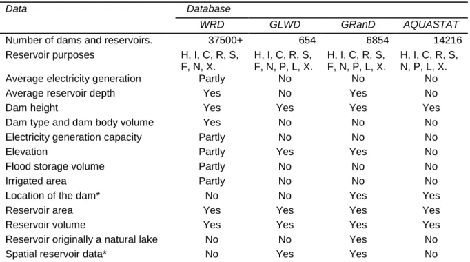
Reservoir data is provided by several reservoir databases (table 2.1.). The most common reservoir databases are: the world register of dams (WRD), provided by the international commission of large dams (ICOLD, 2011), the global dams and reservoirs database (GRanD), provided by Lehner et al. (2011), the global lakes and wetlands database (GLWD), provided by Lehner and Döll (2004) and the dam database provided by AQUASTAT (FAO, 2015). However, the reservoir part of the GLWD is based on the GRanD database.

Table 2.1. The available data per reservoir database.

Data Database

WRD GLWD GRanD AQUASTAT

Number of dams and reservoirs. 37500+ 654 6854 14216

Reservoir purposes H, I, C, R, S, F, N, X.

H, I, C, R, S, F, N, P, L, X.

H, I, C, R, S, N, P, L, X.

Average electricity generation Partly No No No

Average reservoir depth Yes No Yes No

Dam height Yes Yes Yes Yes

Dam type and dam body volume Yes No No No

Electricity generation capacity Partly No No No

Elevation Partly Yes Yes No

Flood storage volume Partly No No No

Irrigated area Partly No No No

Location of the dam* No No Yes Yes

Reservoir area Yes Yes Yes Yes

Reservoir volume Yes Yes Yes Yes

Reservoir originally a natural lake No No Yes No

Spatial reservoir data* No Yes Yes No

For the reservoir purposes: H: Hydro energy, I: Irrigation, C: Flood prevention, R: Recreation, S: Industrial and residential water supply, F: Commercial fishing, N: Navigation, P: Pollution control, L: Livestock water supply, X: Other. *: The difference between the location of the dam and spatial reservoir data is the spatial reservoir data provides the borders of the reservoir while the dam location is only a single point.

(25)

25

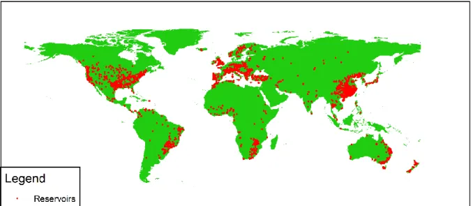
None of the reservoir databases is complete and if data for a reservoir was not available in the WRD database, but is available in the GRanD database, then information from the GRanD database was used. Based on information from the GranD database, reservoirs with a natural origin were excluded from the database. However, most reservoirs with a natural origin are still in the database, because there is no proper information about this subject in both databases. Also river and coastal barrages were excluded, because these structures do not actually store water. Totally, this resulted a usable database of 5502 reservoirs. However, not all required economic data was available for these 5502 reservoir and the final reservoir database only includes 2235 reservoirs with full data availability. The location of these reservoirs is shown in figure 2.1. This corresponds to 3,8% of the reservoirs available in the WRD database and to 30,1% of the total reservoir volume of all reservoirs in the WRD database.

Figure 2.1. The location of the 2235 reservoirs globally.

2.2. Methodology and data to determine the economic value of reservoirs

It is common for a reservoir to have multiple purposes and within the water footprint concept, the water use is allocated to each purpose based on economic value of each purpose. This paragraph describes how the economic value of reservoirs is determined and gives the allocation coefficients to attribute the water use to each reservoir purpose.

The most common reservoir purposes are: generate hydro-electricity, supplying water for residential and industrial use, supply irrigational water, regulate the flow of rivers to prevent flooding and enable inland navigation (U.S. Army Corps of Engineers, 1997; International Commission on Large Dams 2000). Reservoirs are rarely created for recreational and fishing purposes, but after creation these are important secondary purposes (Ward, et al., 1996; Weinin, et al., 2006). Other rare reservoir purposes are pollution control and life stock feeding (Lehner, et al., 2011). In this study navigation is neglected as purpose, because before the reservoir was constructed, the river could have a navigation function. Other purposes are neglected because they are unspecified in the WRD database. The total economic value per reservoir is the sum of the economic value of all reservoir purposes.

(26)

26 2.2.1. The economic value of hydropower generation

The generation of electricity is one of the most common reservoir purposes. Energy generated by hydropower plants in considered as renewable energy and hydropower production is the largest supplier of renewable energy (ICOLD, 2000). The economic value of hydropower generation per reservoir is determined, by multiplying the mean annual electrical generation per reservoir (in GWhy-1_{), with the}

economic value of electricity per country (in $kWh-1_).

The WRD database provides the mean annual electricity generation and the production capacity for 984 reservoirs and for another 359 reservoirs, only the production capacity is available. For reservoirs with only the production capacity, the assumption is made that these reservoirs are generating energy 34% of the time on full production capacity. This percentage is based average productivity/production capacity ratio of the first 984 reservoirs. Prices for electric energy are provided by Eurostat (2015), RCREEE (2013), IEA (2012), Statista or local sources for different years (Appendix B). If the electricity price is not available for a country, then prices of neighbouring countries are used to determine an average price for that nation.

2.2.2. The economic value of irrigation water supply

Irrigation water storage is the most common reservoir purpose and globally 48 percent of the reservoirs have this function (ICOLD, 2011). The irrigated area per reservoir (ha) is provided by the WRD database for 763 reservoirs. The economic value of irrigation water supply by reservoirs is determined by multiplying the irrigated area per reservoir with the average economic value of agriculture land per hectare per country ($ha-1_y-1_).

The average economic value of agricultural land is determined per nation, based on the value of annual agricultural production per crop (in $unit of production-1_y-1_{) and the annual harvested area per crop (ha).}

Both are provided by FAOstat (2015) until the year 2013. Based on the values per crop, one average annual value per hectare per nation is determined. The annual average economic value per hectare per nation are shown in appendix C. Assumed is that the economic value of irrigated land is fully depended of irrigation water.

2.2.3. The economic value of flood control storage

Dams and reservoirs are an effective measure to regulate water levels in rivers and prevent flooding by storing the discharge peaks (ICOLD, 2011). This study only accounts the economic value of flood prevention, because it is not possible to determine the economic value of water level regulation. The economic value of flood prevention is determined by multiplying the available flood storage volume with the economic value of flood storage. The WRD database provides for 648 reservoirs the available flood storage capacity (m3_).

The economic value of flood storage capacity is based on the prevented damage by 23 dams, constructed between 1941 and 1972 in the United states. Annually, the economic value of flood storage capacity for these reservoirs varies between $0,002 to $0,58 per cubic meter, with an average of $0,117/m3_y-1_{(appendix D). This is of the same order of magnitude to the value of $0,16 per m}3_provided

by Zhoa and Liu (2015) for the Three Gorges reservoir. The determined economic value is used for all reservoirs globally that have flood control as stated purpose.

2.2.4. The economic value of residential and industrial water supply

There is a large variation in the volume of water supplied by nature and to prevent residential and industrial water shortages, water is often stored in reservoirs. The economic value of residential and industrial water supply by reservoirs is determined by multiplying the estimated annual abstracted volume (m3_y-1_{) with the economic value of residential water per country ($m}-3_{). Water supply prices per}

cubic meter are provided Danilenko et al. (2014), IWA (2012) and the OECD (2010) for different years. If for a certain country the price is not available, then prices of neighbouring countries are used to determine an average price for that nation. The used prices are given in appendix E.

(27)

27

volume and climate. Small reservoirs in humid climates have a generally high abstraction/volume ratio, while large reservoirs located in arid climates have generally small ratio. Based on these ratios, two exponential formulas, one for humid climates and one for arid climates, are used to estimate the volume abstracted from reservoirs (appendix F).

2.2.5. The economic value of recreation

All over the world, open water is used for recreation (Costanza, et al. 1997). Open water provided by reservoirs are used for swimming, sailing, motor boating, water skiing and recreational fishing (Ward et al., 1996; Bhat et al., 1998). The economic value of recreation is determined by multiplying the economic value of recreation with the reservoir surface. Several scientific sources provide the economic value of open water recreation. However, only the economic value provided per square meter is useful and this is only provided by Costanza, et al. (1997), which gives a value of $230y-1_{for open water recreation per}

hectare in 1994 U.S.$. This value is used globally because better data is not available. The reservoirs area per reservoir is provided by ICOLD (2011).

2.2.6. The economic value of commercial reservoir fishing

Besides recreational fishing, commercial fishing is an important secondary reservoir purpose. Reservoir facilitate both aquaculture and traditional wild catch fishing (Weimin et al., 2006; van Zwieten, et al., 2011) with aquaculture have a far higher yield compared to traditional fishing. However, the aquaculture yields are not applicable to most reservoirs globally and therefore only wild catch fishing yields are used. Yields are provided per nation for all caught species. The economic value of commercial reservoir is determined by multiplying the fishing yield (kgha-1_yr-1_{) with the reservoir area (ha) and the average price}

of fresh water fish ($kg-1_{). The reservoir area is provided by ICOLD (2011). Both the fishing yield and}

average price per fresh water fish is provided by multiple sources (appendix G). 2.2.7. Allocation coefficients

For reservoirs with only a single purpose, the amount of evaporation is fully contributed to this purpose. When a reservoir has multiple purposes, an allocation coefficient is required to divide the amount of evaporation among the purposes (equation 2.1).

𝜂𝑖= 𝑉𝑖

Σ𝑉𝑖 (2.1)

Where ηi is the allocation coefficient and Vi is the economic value of a purpose. The sum of all economic

values per purposes gives the total economic value of all reservoir purposes.

2.3. Method and data to estimate the evaporation from reservoirs

The evaporation from the 2235 reservoirs with allocation coefficients is determined in four different ways: with a method provided by Kohli and Frenken, with the method of Jensen and Haise, with the method of Hamon, and with a modified version of the Penman method. None of the used methods includes the thermal heat storage in reservoirs, which can result in a deviation in the determined evaporation figure (Finch, 2001). With each of these methods the evaporation is determined on a daily basis. If the daily evaporation was negative, then the evaporation figure was set to zero (Finch & Hall, 2001). The annual reported evaporation is the sum of the daily evaporation for 365 days. The evaporation per reservoir is the average of the annual evaporation determined with the 4 used methods. Each evaporation method is described below together with the used climate data.

2.3.1. The method by Kohli and Frenken

Based on data from the FAO global evapotranspiration map (2004) the evaporation is determined using equation 1.1. The assumed the crop coefficient for open water is 1, this gives an evaporation in mmy-1_.

With ArcGIS, the annual evapotranspiration was determined for the midpoints of each reservoir. 2.3.2. The method of Jensen and Haise

(28)

28

distant climate station (Winter, et al., 1995; Rosenberry, et al., 2007 and Majidi, et al., 2015). It is an energy budget method and the evaporation is estimated based on solar radiation and average daily temperature, for a minimal period of 5 days (Jensen & Haise, 1963). However, it is also possible to use is for shorter periods of minimal 1 day (Rosenberry, et al., 2007 and Majidi, et al., 2015). The method of Jensen and Haise is given by equation 2.2 (Majidi, et al., 2015).

𝐸𝑑= 0,03523𝑅𝑠(0,014𝑇𝑎− 0,37) (2.2)

Where E is the amount of evaporation in mmday-1_{, R}_s_{is the incoming solar radiation in Wm}-2 _{and T}_a_the

mean daily temperature in F°. If the mean daily temperature is lower than -3,06 °C (26,5 °F) the evaporation becomes negative and the negative daily evaporation figures were set to zero. With Rs in MJm-2_d-1 _{, T}

a in °C and with a minimal daily temperature, the equation of Jensen and Haise becomes:

𝑖𝑓 𝑇𝑎 ≥ −3,06 °𝐶 𝑡ℎ𝑒𝑛 𝐸 = 0,4087𝑅𝑠 (0,014 ((1,8𝑇𝑎) + 32) − 0,37) (2.3) 𝑖𝑓 𝑇𝑎 < −3,06 °𝐶 𝑡ℎ𝑒𝑛 𝐸 = 0

The evaporation was determined per reservoir on a daily basis and the daily figures where summed to an annual evaporation. The required input variables are the mean air temperature and the incoming solar radiation. Equations to determine the incoming solar radiation are provided by appendix H.

2.3.3. The method of Hamon

The method of Hamon (1961) was developed to estimate evapotranspiration on a daily basis, based on the relation between the maximal incoming energy and the moisture capacity of the air (Hamon, 1961; Harwell, 2012; Majidi, et al., 2015). Assumed is that the evaporation from open water is equal to evapotranspiration and a modified version of this method is used within the U.S. Army Corps of Engineers, to estimate evaporation from reservoirs (Harwell, 2012). Equation 2.4 presents the Hamon methods as used to determine daily evaporation in millimetres (Schertzer & Taylor, 2009; Harwell, 2012; Majidi, et al., 2015).

𝐸𝑑= 13,97 ( 𝑁 12)

2 (𝑆𝑉𝐷

100) (2.4)

Where E is the daily evaporation in mm, N is the maximal number of daylight hours, and SVD is the saturation vapour density in gm-3_{. Equations to determine the maximal number of daylight hours and the}

saturation vapour density are provided by appendix H. 2.3.4. The modified Penman method

Penman was the first to combine the mass transfer and energy budget methods (Shaw, 1994; Majidi, et al., 2015). This elimated the need of the surface water temperature to determine the evaporation from open water. In this study, a modified version of the Penmen equation is used. This version was developed by the U.S. weather bureau to estimate lake evaporation based on evaporation from pans (Kohler, et al, 1955; Harwell, 2012). The daily evaporation is estimated based on the average daily air temperature, the average daily windspeed at 10 meter, the dewpoint temperature and solar radiation. Kohler et al. (1955) assumed that the energy storage in reservoirs does not influence the amount of evaporation from reservoirs. Equation 2.5. presents the modified Penman method (Harwell, 2012).

𝐸𝑑= 0,7 ( Δ

Δ + 𝛾 𝑅𝑛+ 𝛾

(29)

29

Where E is the daily evaporation in mm, ∆ is the gradient of saturated vapour pressure, γ is the psychrometric constant, Rn is the effective net radiation in mmd-1, Ea is the amount of evaporation from

a Class A pan in mmd-1_{. Equations to determine the effective net radiation and the evaporation from a}

Class A pan are provided by appendix H. 2.3.5. Climatological data

Climatological data were obtained from the ERA Interim database (Dee, et al., 2011) with a resolution of 0,5 arc minute for the years 1981-2010. The 4 hourly data was averaged to daily figures, because not all variables were available on the same time step. Secondly, one daily average was determined for the 1981-2010 period. Values on mean air temperature, dew point temperature, wind speed in U and V direction and the actual hours of sunshine were obtained for the midpoints point of all 2235 reservoirs. These reservoir midpoints were determined using ArcGIS and for not all reservoirs the midpoint was located on the water surface. Reservoir attitude, reservoir depth and reservoir area were obtained from the combined WRD and GRanD databases.

The global evapotranspiration map to estimate the reference evaporation was obtained from the FAO (2004) with a resolution of 10 arc minute. The evapotranspiration was determined with ArcGIS, using the reservoir midpoints.

2.4. Method and data to determine the water footprint related to reservoir construction

The water footprint of reservoir construction depends mainly on the construction material of the dam. Earth and rock fill dams are mainly constructed with material that is found in the surrounding area of the construction site (Novak et al., 2007; Chen, 2015). Gravity, buttress and arc dams are mainly constructed of reinforced concrete. Other aspects of reservoir construction like removal of trees and other objects from the reservoir zone are neglected, because the water use during these activities is relatively low.

The water footprint of embankment dams depends mainly on the energy used to excavate the used rock or earth. These materials are excavated in the surrounding area of the construction site (Novak, et al., 2007; Chen, 2015). The assumption is made that the excavation site is located on an average distance of 20 km from the construction site. No useful data is available about the fuel use during excavation works, but one study is done to the CO2 emissions during excavation works (Ahn, et al., 2009).

During this study 4747 m3_{of earth was excavated, moved over 1 km and dumped with a total emission}

of 1700 kg CO2. Diesel is the main fuel used in the construction industry (Ahn, et al., 2009). On average,

the CO2 emission from 1 litre fuel is 2,65 kg (ACEA, 2013), which means that on average, 0,15 l fuel is

used to move 1 m3_{of earth over a distance of 1 km. The water footprint of crude oil is 1058 m}3_/MJ

(Gerbens-Leenes, et al., 2008). Diesel has a calorific value of 45,5 MJkg-1_{(ACEA, 2013) and a density}

of 0,84 kgl-1_{(ISO, 1998), so the water footprint of diesel is 40 l/l. This gives an estimated water footprint}

for earth or rock moving operations of 6 lkm-1_m-3_{. For earth or rock that is excavated 20 km from the}

construction site, the water footprint is 0,12 m3_/m3_.

Gravity, arc and buttress dams have reinforced concrete as their main construction material. Reinforced concrete is a composite material composed of cement, steel and aggregates. Bosman (2016) gives for Portland cement a water footprint of 415 m3_/m3_{and the water footprint for unalloyed steel is 18254}

m3_/m3_{. For the aggregates, the water footprint of earth and rock are used. Assumed is that the concrete}

used in dams, exists out of 1 % steel, 29 % cement and 70 % aggregates, this gives a water footprint of 303 m3_/m3_.

(30)

30

If the dam volume was not available for a certain dam in the database, then the volume of the dam body was estimated based on the dam height and a factor based on the dam construction type (embankment, gravity, buttress or arch dam). The dam type factor is the ratio between the dam volume and the dam height and based on the ratios of the dams with an available dam volume and dam height (appendix I). Table 2.2. gives for all dam types the main construction material and the dam type factor. The dam types are provided by ICOLD (2011).

The water footprint of dam construction is the volume of the dam body multiplied with the water footprint of the construction material. Earth and rock filled dams have in most cases a filter or a concrete element to make the dame water tight (Novak et al., 2007; Chen, 2015). These concrete elements are neglected because no data is available about the volume of these elements.

Table 2.2. Construction material and the dam typed factor to estimate the dam volume.

Dam type Construction material Dam type factor

Embankment dam, earth fill Earth 71038

Embankment dam, rock fill Rock 35177

Gravity dam Reinforced concrete 18027

Buttress dam Reinforced concrete 6970

Arch dam Reinforced concrete 2874

2.5. Method to determine the water footprint related to reservoir operation

The water footprint approach described by Hoekstra, et al. (2011) is used to determine the water footprint of reservoir products. Based on the evaporation per reservoir, the annual blue water footprint related to evaporation (WFE) is determined using equation 2.6. Were Ey is the mean evaporation in mmy-1 and A

is the reservoir area in ha. Because the area corresponds the maximal reservoir volume, a factor κ is used to correct the reservoir area, to resemble average filling conditions. In this study, κ has a value of 0,5625 and this value is determined in appendix L.

𝑊𝐹𝐸= 10 × 𝐸𝑦× 𝐴 × 𝜅 (2.6)

To determine the water footprint of a certain product, the whole production process should be taken into account (Hoekstra, et al., 2011). This means that for reservoir products, the water footprint of reservoir construction should be included. So, the total water footprint per reservoir (WFt) is the sum of the blue

water footprint related to evaporation (WFE) and the water footprint related to reservoir construction

(WFC). This is presented in equation 2.7. The annual water footprint related to reservoir construction is

determined per reservoir in paragraph 2.4.

𝑊𝐹𝑡= 𝑊𝐹𝐸+ 𝑊𝐹𝑐 (2.7)

According to the water footprint approach, the water footprint related to a production process should be allocated to each of the products, based on its economic value (Hoekstra, et al., 2011). So, when a reservoir has only one purpose, then the water footprint is totally contributed to that purpose. When a reservoir has multiple purposes, the water footprint is allocated to each purpose based on its economic value. This method is presented in equation 2.8, where WFP is the water footprint per purpose and ηp is

(31)

31

𝑊𝐹𝑝= 𝑊𝐹𝑡 × 𝜂𝑖 (2.8)

2.6. Method to determine the water footprint related to reservoir operation in the context of water scarcity

Water that evaporates from reservoirs will no longer be available for use downstream of the reservoir. This can make water scarcity more serious, in river basins with already water scarcity problems. Reservoirs with the purposes irrigation water supply and residential and industrial water supply, increase the availability of water in the dry season (Bakken et al., 2015). Secondly, reservoirs prevent flooding by managing the water level in the wet seasons. Reservoirs are the only available ‘tool’ to provide these products and services and therefore, they are considered as needed (Bakken et al., 2015). Reservoirs with the purposes hydropower generation, recreation and commercial fishing are considered as not needed purposes, because there are alternative ways to produce energy, food or to provided recreational services.

(32)

32

3. Results

In this chapter, the results are presented per sub question. So, in the first paragraph the results are presented of the economic study. In the second paragraph the results are presented of the evaporation part of this study. The third paragraph presents water footprint related to reservoir operation. In the last paragraph, the water foot print related to reservoir operation in the context of water scarcity is presented.

3.1. Economic value of reservoirs and allocation coefficients

The total annual economic value of the reservoirs in this study are $ 311 billion in 2014 U.S. dollars. In table 3.1. the total economic value and allocation coefficients are presented per continent. In general, most economic value is generated by hydropower generation, irrigation water supply and residential and industrial water supply. Interesting is the low economic value of the reservoirs in this study in North America compared to the number of reservoirs. Table 3.2. shows the total economic value and allocation coefficients for 11 selected reservoirs.

Table 3.1. The total annual economic value and allocation coefficients per continent and globally. Number of

reservoirs

Total economic Allocation coefficients per purposes

value (mln US$y-1₎ _H _I _P _R _S _F

Africa 203 $20.064 19% 15% 30% 0,0% 36% 0,0%

Asia 653 $93.539 21% 52% 17% 0,1% 10% 0,9%

Europe 519 $53.708 19% 3% 13% 0,0% 65% 0,0%

North America 549 $30.686 20% 0% 0% 0,7% 80% 0,0%

Oceania 171 $24.684 9% 3% 0% 0,0% 88% 0,0%

South America 140 $88.135 77% 0% 1% 0,1% 22% 0,0%

Global 2235 $310.818 35% 17% 9% 0,1% 38% 0,3%

For the reservoir purposes: H: Hydro energy, I: Irrigation water supply, P: Flood prevention, R: Recreation, S: Industrial and residential water supply, F: Commercial fishing

Table 3.2. The total annual economic value and allocation coefficients per purpose, for 11 selected reservoirs.

Dam or reservoir name Total economic Allocation coefficients per purposes

value (mln US$y-1₎ _H _I _P _R _S _F

Arapuni $ 90 85% 15%

Finchaa $ 20 100%

Guri $ 1.612 100%

Lake Mead $ 713 85%1 _0% _15%

Itaipu $ 7.560 100%

Kariba $ 576 100%

Kulekhani $ 14 100%

Lake Nasser $ 8.031 4% 28% 68%

Nam Ngum $ 35 100%

Sayano-Shushenskaya $ 1.279 100%

Three Gorges $ 6.907 51% 37% 0% 9% 3%

For the reservoir purposes: H: Hydro energy, I: Irrigation water supply, P: Flood prevention, R: Recreation, S: Industrial and residential water supply, F: Commercial fishing. 1_{: The WRD does not gives data hydropower}

(33)

33

The results for the Three Gorges reservoir are compared with the annual averaged economic value and allocation coefficients available for this reservoir (Zhoa & Liu, 2015). This is the only comparable study, were the economic value per reservoir purpose is known. According to the WRD database, the reservoir purposes of the Three Gorges reservoir are hydropower generation, irrigation, flood control storage and commercial fishing. This does not correspond to the purposes gives by Zhoa and Liu (2015). So, the purposes provided by Zhoa and Liu (2015) are used, because this gives an opportunity to compare the results. For the purposes hydropower generation, flood control storage and commercial reservoir fishing, the determined annual economic value are within the range of the “real” economic value (figure 3.1). The economic value of recreation is underestimated, which is probably caused by the used global average economic value of open water recreation. The economic value of residential and industrial water supply is heavily overestimated, which is mainly caused by relatively low water supply abstraction from the Three Gorges reservoir compared to the size. The determined total economic value of the Three Gorges reservoir is of the same order of magnitude as the total economic value determined by Zhoa and Liu (2015).

Figure 3.1. The modelled and annual economic value per purpose for the reservoir of the Three Gorges dam, provided by Zhoa and Liu (2015). Zhoa and Liu presents the economic value for multiple years. Therefore a minimum and a maximum economic value is given. The minimum economic value for flood control storage and residential and industrial water supply is $0,-. The total economic value provided by Zhoa and Liu includes also the economic value of navigation on the three Gorges dam.

3.2. Evaporation from reservoirs

The total annual evaporation volume from the 2235 reservoirs in this study is 1,04 x 1011_m3_{. Table 3.3.}

shows the minimal, mean and maximal total evaporation volumes from reservoirs in this study per continent. The mean total evaporation volume is the mean of the four used evaporation methods, while the minimal and maximal evaporation volume are provided by a single method. For all continents, the minimum evaporation volume is determined with the method of Hamon and the maximal evaporation volume is determined by the Penmen method.

In table 3.4 the evaporation figures for 11 selected reservoirs are presented for each used evaporation method, as average of these methods and together with evaporation figures from the literature. From most of the selected reservoirs, the evaporation provided by the literature is of the same order of

$1.000.000 $10.000.000 $100.000.000 $1.000.000.000 $10.000.000.000

Hydropower generation

Flood control storage

Recreation Residental and industrial

water supply

Commercial fishing

Total

E

c

on

im

ic

v

al

ue

pe

r

y

ea

r

Economic value Zhoa & Liu Modelled economic value

Maximum

(34)

34

magnitude as the determined evaporation figures. Exceptions are Lake Mead, the Kariba dam and the Three Gorges dam.

Table 3.3. The evaporation volume from reservoirs per continent and globally. Minimal evaporation

volume (109_m3_y-1₎

Mean evaporation volume (109_m3_y-1₎

Max evaporation volume (109_m3_y-1₎

Africa 19,7 28,9 38,7

Asia 16,2 22,4 30,4

Europe 2,4 2,7 3,4

North America 4,0 6,2 7,9

Oceania 1,5 2,2 2,8

South America 27,8 42,0 55,0

Global 76,1 104,4 138,2

Table 3.4. The reservoirs evaporation for 11 selected reservoirs. Dam or

reservoir name

Evaporation in mmy-1 Kohli &

Frenken

Jensen-Haise

Hamon Penman Mean Literature

(table 2.2)

Arapuni 755 843 624 944 792 844

Finchaa 1340 1572 826 1765 1376 1650

Guri 1556 2407 1210 2524 1924 2042

Lake Mead 1013 1086 661 1334 1024 1652a

Itaipu 1248 1903 1042 1988 1545 1808

Kariba 1693 2017 1212 2666 1897 2860

Kulekhani 1032 1799 910 2181 1481 1574

Lake Nasser 2643 2152 1435 3947 2544 2350a

Nam Ngum 1362 2149 1114 2114 1685 1710a

Sayano -Shushenskaya

584 427 363 622 499 486

Three Gorges 875 1233 767 1257 1033 685

a_{: average of the minimal and maximal values from table 2.2}

Figure 3.2. The average evaporation per climate Köppen-Geiger climate class (Kottek, et al., 2006), for the four used evaporation methods. The main climates classes are shown below the climate classes.

0 500 1000 1500 2000 2500 Af

Am As Aw

B W k B W h B S k B S h C fa C fb C fc C s a C s b

Cwa Cwb D

fa D fb D fc D s a D s b D s c

Dwa Dwb Dwc ET

Ev a p o ra ti o n i n m m y -1

(35)

35

Figure 3.2 shows the average evaporation per climate Köppen-Geiger climate class (Kottek, et al., 2006), for the evaporation methods used in this study. In general, the modified Penman method gives the highest evaporation figures, while the Hamon method produces the lowest evaporation figures. It is known that the original Hamon method tends to underestimates the evaporation (Harwell, 2012; Majidi, et al., 2015). For warm arid climates (BWh and BWk) the modified Penman gives very high evaporation figures compared to the other used methods. This is also visible in the evaporation values for lake Nasser in table 3.4. The method of Jensen and Haise gives high evaporation figures for equatorial climates (Af to Aw). A possible reason for this is that this method was originally developed for more arid regions (Jensen & Haise, 1963).

Figures 3.3. to 3.5. show for three individual reservoirs, the monthly evaporation determined with three evaporation methods and compares it with literature data. The method of Kolhi and Frenken is not used because it gives only annual evaporation data. Reservoirs are selected based on data availability in both the literature and the used reservoir database. For the reservoir of the Guri dam (figure 3.3.), the evaporation data is provided by Códova (2006) for the year 2002. For the whole year the evaporation provided by Códova (2006) is located between the higher and lower evaporation estimations.

Figure 3.3. The monthly evaporation for the reservoir of the Guri dam per evaporation method, these figures are compared with evaporation figures provided by Códova (2006) for the year 2002.

Figure 3.4. The monthly evaporation for lake Mead per evaporation method, these figures are compared with evaporation figures provided by Moreo and Swancar (2013) for the year 2012.

50 100 150 200 250

Jan Feb Mar Apr May Jun Jul Aug Sep Oct Nov Dec

Ev a p o ra ti o n i n m m p e r m o n th

Jensen-Haise Hamon Penman Códova (2006)

0 50 100 150 200 250

Jan Feb Mar Apr May Jun Jul Aug Sep Oct Nov Dec

Ev a p o ra ti o n i n m m p e r m o n th