Abstract—Suppliers and manufacturers recognize the importance of interactions between financial and inventory decisions in the development of effective supply chains.
Moreover, achieving effective coordination among the supply chain players has become a pertinent research issue. This paper considers a two-echelon model, consisting of multi-suppliers and one manufacturer, coordinating their situations to maximize the total supply chain profits. Each supplier supplies one or more components required in the final product produced. In the proposed inventory level model, the permissible delay in payments is coordinated to order quantity between two echelons.
Index Terms—Assemble, Permissible delay in payment, Two-echelon model
I. INTRODUCTION
A supply chain consists of different facilities where raw materials, intermediate products, or finished products are purchased, produced, or stored. In today’s economy, many companies do not have all technical and organizational skills to efficiently satisfy the demand of customers.
Therefore, they try to identify the business processes they can conduct efficiently. To manage these facilities like one company, the products, cash, or information flow should be integrated.
In assemble-to-order systems, suppliers send assembled items to the manufacturer when they receive order forms.
Hillier[1] indicated that replacing some specific components by a smaller number of common components can reduce safety stock levels due to the benefits of risk pooling. He developed a model to consider the assemble-to-order environment where components were replenished according to a (Q,r) policy. Ervolina et al.[2]
proposed a novel availability management process called Available-to-Sell (ATS) that drives a better supply chain efficiency. The substitution of higher-class components for Ming-Cheng Lo is with Department of Business Administration, Chien Hsin University of Science and Technology, No.229, Jianxing Rd., Zhongli City, Taoyuan County 32097, Taiwan, R.O.C. (e-mail: [email protected])
Ming-Feng Yang* (Corresponding Author) is with Department of Transportation Science, National Taiwan Ocean University, No.2, Beining Rd, Jhongjheng District, Keelung City 202, Taiwan, R.O.C. (phone:
+886-2-24622192#7011;fax:+886-2-24633745;e-mail:[email protected] ou.edu.tw)
Tse-Shuan Hung (Corresponding Author) is with Department of Transportation Science, National Taiwan Ocean University, No.2, Beining Rd, Jhongjheng District, Keelung City 202, Taiwan, R.O.C. (e-mail:
Su-Fang Wang is with Department of Transportation Science, National Taiwan Ocean University, No.2, Beining Rd, Jhongjheng District, Keelung City 202, Taiwan, R.O.C. (e-mail: [email protected])
lower one was often applied when the latter are stock-out.However, the decision for substitution should be made in advance. Iravani et al.[3] considerd an assemble-to-order system where each customer order consists of a mix of key and non-key items. Reiman and Wang[4] introduced a multi-stage stochastic program that provides a lower bound on the long-run average inventory cost. The stochastic program also motivates a replenishment policy for these systems. Recently, Chang et al.[5]
considerd a two-stage assembly system with imperfect processes. Danilovic et al.[6] proposed a new optimization approach to address a multi-period, inventory control problem under stochastic environment. Elhafsi et al.[7]
studied a assembled model serving both the demand of end products and the individual components.
Permissible delay in payment is a brand-new issue. The different between a traditional model and a new one is that the buyer must pay immediately when the vendor delivers products to the buyer in a traditional EOQ model. And in the model with permissible delay in payment, the vendor usually gives a fixed period to reduce the stress of capital.
During the period, the buyer can keep products without paying to the vendor and earns extra interest from the sale.
Jaber and Osman[8] proposed a centralized model where players in a two-level supply chain coordinate their orders to minimize their local costs. Pal et al.[9] investigated the optimal replenishment lot size of supplier and optimal production rate of manufacturer under three levels of trade credit policy. In 2013, Chiu and Yang et al.[10] developed an improved inventory model which helps the enterprises to advance their profit increasing and cost reduction in a single vendor-single buyer environment depending on the ordering quantity and imperfect production. For more closely conforming to the actual inventories and responding to the factors that contribute to inventory costs, they proposed model can be the references to the business applications.
Das et al.[11] developed a multi-item inventory model with deteriorating items for multi-secondary warehouses and one primary warehouse. Items were sold from the primary warehouse which is located at the main market. If the stock level were numerous that there are insufficient space of the existing primary warehouse, then excess items will store at multi-secondary warehouses of finite capacity. Sarkar et al.[12] assumed a policy along with the production of defective items where the order quantity and lead time are considered as decision variables. Chen and Teng [13]
proposed an EOQ model for a retailer when: (1) her/his product deteriorates continuously, and has a maximum lifetime, and (2) her/his supplier offers a permissible delay in payments. Yang and Tseng[14] proposed a three-echelon inventory model with permissible delay in payments under
Integrated Assembled Production Inventory Model
M.C. Lo, M.F. Yang*, T.S. Hung and S.F. Wang
controllable lead time and backorder consideration to find out the suitable inventory policy to enhance profit of the supply chain. In the next year, Yang et al.[15] added defective production and repair rate to the proposed model and discussed how these factors may affect profits. In addition, holding cost, ordering cost, and transportation cost will also be considered as they develop the integrated inventory model with price-dependent payment period under the possible condition of defective products. Finally, this research consists of multi-suppliers and one manufacturer in the ATO system under the permissible delay in payment which coordinates their situations to minimize the total supply chain costs.
II. NOTATIONS AND ASSUMPTIONS
In order to develop the two levels inventory model with assemble system and permissible delay in payment. We divide some notations of the expected joint annual inventory model in two parts which are the annual profit of multi-suppliers and one manufacturer. The notations and assumptions as below are used in this two levels inventory model:
A. Notations
Q = Manufacturer’s economic quantity, a decision variable.
ns = The number of lots delivered in a production cycle from the s𝑡ℎ supplier to the manufacturer, a positive integer, a decision variable.
Supplier side
Q𝑠 = Economic deliverycomponent quantity of each supplier, where Q𝑠= Q ∗ ∑ u𝑖 𝑠𝑖.
P𝑠 = The 𝑠𝑡ℎ Supplier’s production rate.
Ds = Average annual demand per unit time of each supplier.
C𝑠𝑖 = Supplier’s purchasing cost for item i per unit.
A𝑠 = Supplier’s ordering cost per order.
F𝑠𝑖 = Supplier’s transportation cost for item i per order.
h𝑠𝑖 = Supplier’s holding cost for item i per unit.
I𝑠𝑝 = Supplier’s opportunity cost per dollar per year.
I𝑠𝑒 = Supplier’s interest earned per dollar per year.
Ts = Supplier’s cycle time.
usi = number of units required in one unit of the finished product which supplied by the 𝑠𝑡ℎsupplier.
m = number of suppliers, where s=1,2,…,m.
k𝑠 = number of different types of items supplied by supplier s to the manufacturer, where i=1,2,…, k𝑠. k = number of different types of items supplied by m suppliers. Note that k = ∑𝑚𝑠=1𝑘𝑠 and each supplier supply unique items.That is supplier specific and never identical amongst suppliers.
Manufacturer side
P𝑚 = Manufacturer’s production rate
= Manufacturer’s assembling rate.
D = Average annual demand per unit time.
C𝑚𝑖 = Manufacturer’s purchasing cost for item i per unit.
C𝑝 = Manufacturer’s selling price per unit.
A𝑚 = Manufacturer’s ordering cost per order.
B = Manufacturer’s assembling cost per unit.
h𝑚𝑖 = Manufacturer’s holding cost for the item i per
unit.
h𝑚 = Manufacturer’s holding cost for finished product per unit.
I𝑚𝑝 = Manufacturer’s opportunity cost per dollar per year.
I𝑚𝑒 = Manufacturer’s interest earned per dollar per year.
X = Manufacturer’s permissible delay period.
n𝑚 = The number of lots delivered in a production cycle from the manufacturer to a retailer, a positive integer.
TP𝑠𝑗 = Supplier’s total annual profit in case j, where j=1,2.
CTP𝑠𝑗 = Collective the total annual profit of all suppliers in case j, where j=1,2.
TP𝑚𝑗 = Manufacturer’s total annual profit in case j, where j=1,2.
𝐸𝐽𝑇𝑃𝑗 = The expected joint total annual profit in case j, where j=1,2.
“j” represents two different cases to the relationship of the supplier’s cycle time and permissible payment period of the manufacturer. The detail will be discussed in the Section 3.
B. Assumptions
In this paper, we assume:
(i) This supply chain system consists of multi-suppliers and a manufacturer.
(ii) The finished product requires k items.
(iii) Demand is deterministic and constant over time.
(iv) Economic delivery quantity multiplies by the number of delivery per production run is economic order quantity (EOQ).
(v) Shortages are not allowed.
(vi) The sale price must not be less than the purchasing cost at any echelon, 𝐶𝑝> ∑ ∑ 𝐶𝑠 𝑖 𝑚𝑖∗ 𝑢𝑠𝑖>
∑ ∑ 𝐶𝑠 𝑖 𝑠𝑖∗ 𝑢𝑠𝑖
(vii) The time horizon is infinite.
III. MODEL FORMULATION
In this section, we discuss and develop the supplier and manufacturer’s model and combine them into an integrated joint inventory model.
A. The supplier’s total annual profit
Supplier s supplies i𝑡ℎ item to the manufacturer and each supplier supplies one or more unique items. We divide a few parts in the supplier’s model which are sales revenue, purchasing cost, ordering cost, transportation cost, holding cost, opportunity cost and interest income. The supplier’s total annual profit consists of the following elements:
(1)Sales revenue = D ∗ ∑ 𝐶𝑖 𝑚𝑖∗ 𝑢𝑠𝑖
(2)Purchasing cost = D ∗ ∑ 𝐶𝑖 𝑠𝑖∗ 𝑢𝑠𝑖
(3)Ordering cost =𝐴𝑄𝑠𝐷
(4)Transportation cost = ∑𝑖𝑛𝑠𝐹𝑄𝑠𝑖∗𝐷 (5)Holding cost = ∑ (ℎ𝑠𝑖∗𝐷2𝑃𝑠𝑄𝑠
𝑠)
𝑖
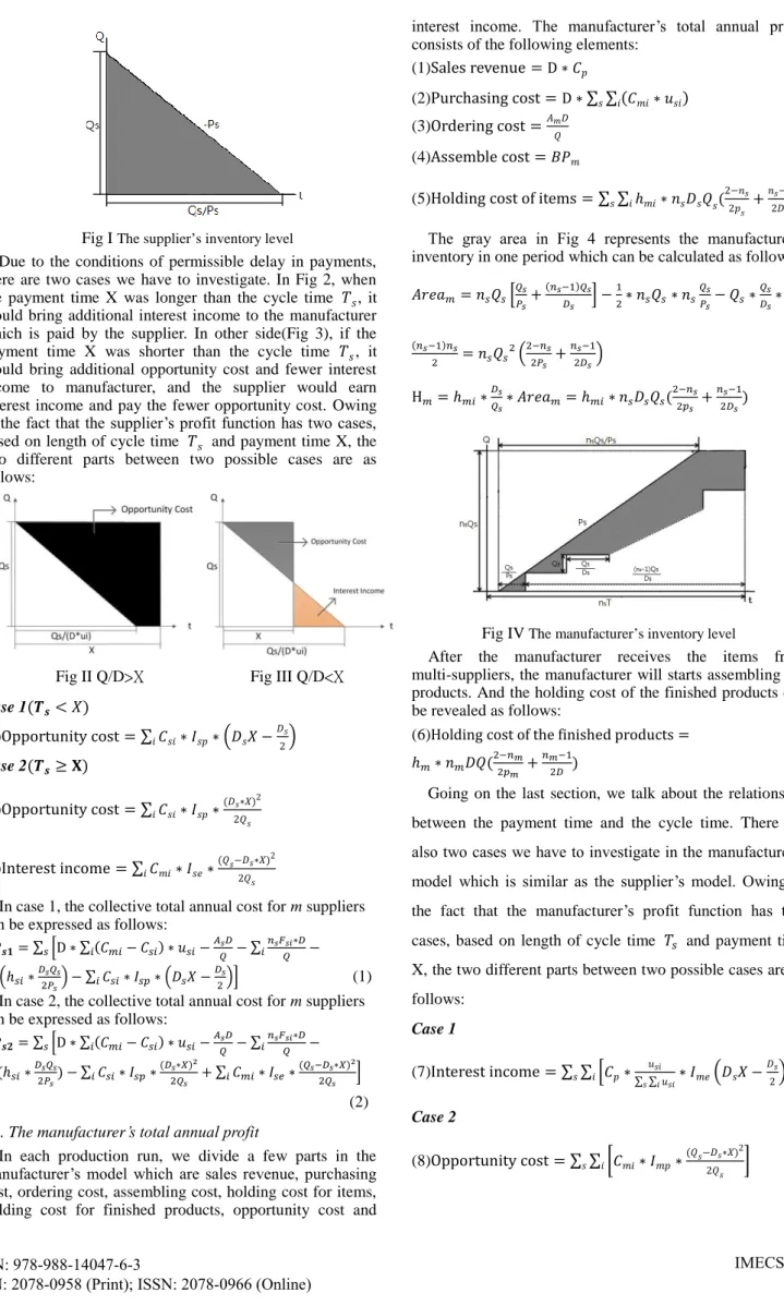
The inventory level of supplier is the black area in Fig1 which can be calculated as follows:
Area𝑠=12∗ 𝑄𝑠∗𝑄𝑃𝑠
𝑠=𝑄2𝑃𝑠2
𝑠 𝐻𝑠= ∑ ℎ𝑖 𝑠𝑖∗𝐷𝑄𝑠
𝑠∗ Area𝑠= ∑ (ℎ𝑠𝑖∗𝐷2𝑃𝑠𝑄𝑠
𝑠)
𝑖
Fig I The supplier’s inventory level
Due to the conditions of permissible delay in payments, there are two cases we have to investigate. In Fig 2, when the payment time X was longer than the cycle time 𝑇𝑠, it would bring additional interest income to the manufacturer which is paid by the supplier. In other side(Fig 3), if the payment time X was shorter than the cycle time 𝑇𝑠, it would bring additional opportunity cost and fewer interest income to manufacturer, and the supplier would earn interest income and pay the fewer opportunity cost. Owing to the fact that the supplier’s profit function has two cases, based on length of cycle time 𝑇𝑠 and payment time X, the two different parts between two possible cases are as follows:
Fig II Q/D>X Fig III Q/D<X Case 1(𝑻𝒔< 𝑋)
(6)Opportunity cost = ∑ 𝐶𝑖 𝑠𝑖∗ 𝐼𝑠𝑝∗(𝐷𝑠𝑋 −𝐷2𝑠) Case 2(𝑻𝒔≥ 𝐗)
(7)Opportunity cost = ∑ 𝐶𝑠𝑖∗ 𝐼𝑠𝑝∗(𝐷2𝑄𝑠∗𝑋)2
𝑖 𝑠
(8)Interest income = ∑ 𝐶𝑚𝑖∗ 𝐼𝑠𝑒∗(𝑄𝑠−𝐷2𝑄𝑠∗𝑋)2
𝑖 𝑠
In case 1, the collective total annual cost for m suppliers can be expressed as follows:
𝑻𝑷𝒔𝟏= ∑ [D ∗ ∑ (𝐶𝑠 𝑖 𝑚𝑖− 𝐶𝑠𝑖) ∗ 𝑢𝑠𝑖−𝐴𝑄𝑠𝐷− ∑𝑖𝑛𝑠𝐹𝑄𝑠𝑖∗𝐷−
∑ (ℎ𝑠𝑖∗𝐷2𝑃𝑠𝑄𝑠
𝑠)
𝑖 − ∑ 𝐶𝑖 𝑠𝑖∗ 𝐼𝑠𝑝∗ (𝐷𝑠𝑋 −𝐷2𝑠)] (1) In case 2, the collective total annual cost for m suppliers
can be expressed as follows:
𝑻𝑷𝒔𝟐= ∑ [D ∗ ∑ (𝐶𝑠 𝑖 𝑚𝑖− 𝐶𝑠𝑖) ∗ 𝑢𝑠𝑖−𝐴𝑄𝑠𝐷− ∑𝑖𝑛𝑠𝐹𝑄𝑠𝑖∗𝐷−
∑ (ℎ𝑠𝑖∗𝐷2𝑃𝑠𝑄𝑠
𝑠)
𝑖 − ∑ 𝐶𝑠𝑖∗ 𝐼𝑠𝑝∗(𝐷2𝑄𝑠∗𝑋)2
𝑖 𝑠 + ∑ 𝐶𝑚𝑖∗ 𝐼𝑠𝑒∗(𝑄𝑠−𝐷2𝑄𝑠∗𝑋)2
𝑖 𝑠 ] (2)
B. The manufacturer’s total annual profit
In each production run, we divide a few parts in the manufacturer’s model which are sales revenue, purchasing cost, ordering cost, assembling cost, holding cost for items, holding cost for finished products, opportunity cost and
interest income. The manufacturer’s total annual profit consists of the following elements:
(1)Sales revenue = D ∗ 𝐶𝑝
(2)Purchasing cost = D ∗ ∑ ∑ (𝐶𝑠 𝑖 𝑚𝑖∗ 𝑢𝑠𝑖) (3)Ordering cost =𝐴𝑚𝑄𝐷
(4)Assemble cost = 𝐵𝑃𝑚
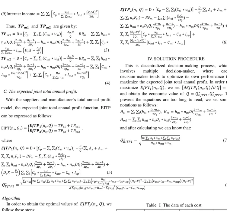
(5)Holding cost of items = ∑ ∑ ℎ𝑚𝑖∗ 𝑛𝑠𝐷𝑠𝑄𝑠(2−𝑛2𝑝𝑠
𝑠 +𝑛2𝐷𝑠−1
𝑠)
𝑖 𝑠
The gray area in Fig 4 represents the manufacturer’s inventory in one period which can be calculated as follows:
𝐴𝑟𝑒𝑎𝑚= 𝑛𝑠𝑄𝑠[𝑄𝑃𝑠
𝑠+(𝑛𝑠−1)𝑄𝐷 𝑠
𝑠 ] −12∗ 𝑛𝑠𝑄𝑠∗ 𝑛𝑠 𝑄𝑠
𝑃𝑠− 𝑄𝑠∗𝑄𝐷𝑠
𝑠∗
(𝑛𝑠−1)𝑛𝑠
2 = 𝑛𝑠𝑄𝑠2(2−𝑛2𝑃𝑠
𝑠 +𝑛2𝐷𝑠−1
𝑠) H𝑚= ℎ𝑚𝑖∗𝐷𝑄𝑠
𝑠∗ 𝐴𝑟𝑒𝑎𝑚= ℎ𝑚𝑖∗ 𝑛𝑠𝐷𝑠𝑄𝑠(2−𝑛2𝑝𝑠
𝑠 +𝑛2𝐷𝑠−1
𝑠)
Fig IV The manufacturer’s inventory level
After the manufacturer receives the items from multi-suppliers, the manufacturer will starts assembling the products. And the holding cost of the finished products can be revealed as follows:
(6)Holding cost of the finished products = ℎ𝑚∗ 𝑛𝑚𝐷𝑄(2−𝑛2𝑝𝑚
𝑚 +𝑛𝑚2𝐷−1)
Going on the last section, we talk about the relationship between the payment time and the cycle time. There are also two cases we have to investigate in the manufacturer’s model which is similar as the supplier’s model. Owing to the fact that the manufacturer’s profit function has two cases, based on length of cycle time 𝑇𝑠 and payment time X, the two different parts between two possible cases are as follows:
Case 1
(7)Interest income = ∑ ∑ [𝐶𝑝∗∑ ∑𝑢𝑠𝑖𝑢
𝑠𝑖 𝑖
𝑠 ∗ 𝐼𝑚𝑒(𝐷𝑠𝑋 −𝐷2𝑠)]
𝑖 𝑠
Case 2
(8)Opportunity cost = ∑ ∑ [𝐶𝑚𝑖∗ 𝐼𝑚𝑝∗(𝑄𝑠−𝐷2𝑄𝑠∗𝑋)2
𝑠 ]
𝑖 𝑠
(9)Interest income = ∑ ∑ [𝐶𝑝∗∑ ∑ 𝑢𝑢𝑠𝑖
𝑠𝑖 𝑖
𝑠 ∗ 𝐼𝑚𝑒∗(𝐷2𝑄𝑠∗𝑋)2
𝑠 ]
𝑖 𝑠
Thus, 𝑻𝑷𝒎𝟏 and 𝑻𝑷𝒎𝟐 are given by:
𝑻𝑷𝒎𝟏= D ∗ [𝐶𝑝− ∑ ∑ (𝐶𝑠 𝑖 𝑚𝑖∗ 𝑢𝑠𝑖)] −𝐴𝑚𝑄𝐷− 𝐵𝑃𝑚− ∑ ∑ ℎ𝑠 𝑖 𝑚𝑖∗ 𝑛𝑠𝐷𝑠𝑄𝑠(2−𝑛2𝑝𝑠
𝑠 +𝑛2𝐷𝑠−1
𝑠) − ℎ𝑚∗ 𝑛𝑚𝐷𝑄(2−𝑛2𝑝𝑚
𝑚 +𝑛𝑚2𝐷−1) + ∑ ∑ [𝐶𝑠 𝑖 𝑝∗
𝑢𝑠𝑖
∑ ∑ 𝑢𝑠 𝑖 𝑠𝑖∗ 𝐼𝑚𝑒(𝐷𝑠𝑋 −𝐷2𝑠)] (3) 𝑻𝑷𝒎𝟐= D ∗ [𝐶𝑝− ∑ ∑ (𝐶𝑠 𝑖 𝑚𝑖∗ 𝑢𝑠𝑖)] −𝐴𝑚𝑄𝐷− 𝐵𝑃𝑚− ∑ ∑ ℎ𝑠 𝑖 𝑚𝑖∗ 𝑛𝑠𝐷𝑠𝑄𝑠(2−𝑛2𝑝𝑠
𝑠 +𝑛2𝐷𝑠−1
𝑠) − ℎ𝑚∗ 𝑛𝑚𝐷𝑄(2−𝑛2𝑝𝑚
𝑚 +𝑛𝑚2𝐷−1) − ∑ ∑ [𝐶𝑠 𝑖 𝑚𝑖∗ 𝐼𝑚𝑝∗(𝑄𝑠−𝐷2𝑄𝑠∗𝑋)2
𝑠 ] + ∑ ∑ [𝐶𝑝∗∑ ∑ 𝑢𝑢𝑠𝑖
𝑠𝑖 𝑖
𝑠 ∗ 𝐼𝑚𝑒∗(𝐷2𝑄𝑠∗𝑋)2
𝑠 ]
𝑖
𝑠 (4)
C. The expected joint total annual profit:
With the suppliers and manufacturer’s total annual profit model, the expected joint total annual profit function, EJTP can be expressed as follows:
EJPT(𝑛𝑠, 𝑄𝑠) = {𝑬𝑱𝑻𝑷𝟏(𝑛𝑠, 𝑄) = 𝑇𝑃𝑠1+ 𝑇𝑃𝑚1 𝑬𝑱𝑻𝑷𝟐(𝑛𝑠, 𝑄) = 𝑇𝑃𝑠2+ 𝑇𝑃𝑚2 , where
𝑬𝑱𝑻𝑷𝟏(𝑛𝑠, 𝑄) = D ∗ [𝐶𝑝− ∑ ∑ (𝐶𝑠 𝑖 𝑠𝑖∗ 𝑢𝑠𝑖)] −𝐷𝑄(∑ 𝐴𝑠 𝑠+ 𝐴𝑚+
∑ ∑ 𝑛𝑠 𝑖 𝑠𝐹𝑠𝑖) − 𝐵𝑃𝑚− ∑ ∑ (ℎ𝑠𝑖∗𝐷2𝑃𝑠𝑄𝑠
𝑠)
𝑖
𝑠 −
∑ ∑ ℎ𝑚𝑖∗ 𝑛𝑠𝐷𝑠𝑄𝑠(2−𝑛2𝑝𝑠
𝑠 +𝑛2𝐷𝑠−1
𝑠)
𝑖
𝑠 − ℎ𝑚∗ 𝑛𝑚𝐷𝑄(2−𝑛2𝑝𝑚
𝑚 +𝑛𝑚2𝐷−1) + (𝐷𝑠𝑋 −𝐷2𝑠) ∑ ∑ [𝐶𝑝∗∑ ∑ 𝑢𝑢𝑠𝑖
𝑠𝑖 𝑖
𝑠 ∗ 𝐼𝑚𝑒− 𝐶𝑠𝑖∗ 𝐼𝑠𝑝]
𝑖
𝑠 (5)
𝑬𝑱𝑻𝑷𝟐(𝑛𝑠, 𝑄) = D ∗ [𝐶𝑝− ∑ ∑ (𝐶𝑠 𝑖 𝑠𝑖∗ 𝑢𝑠𝑖)] −𝐷𝑄(∑ 𝐴𝑠 𝑠+ 𝐴𝑚+
∑ ∑ 𝑛𝑠 𝑖 𝑠𝐹𝑠𝑖) − 𝐵𝑃𝑚− ∑ ∑ (ℎ𝑠𝑖∗𝐷2𝑃𝑠𝑄𝑠
𝑠)
𝑖
𝑠 −
∑ ∑ ℎ𝑚𝑖∗ 𝑛𝑠𝐷𝑠𝑄𝑠(2−𝑛2𝑝𝑠
𝑠 +𝑛2𝐷𝑠−1
𝑠)
𝑖
𝑠 − ℎ𝑚∗ 𝑛𝑚𝐷𝑄(2−𝑛2𝑝𝑚
𝑚 +𝑛𝑚2𝐷−1) +
∑ ∑ (𝐷2𝑄𝑠∗𝑋)2
𝑠 [𝐶𝑝∗∑ ∑ 𝑢𝑢𝑠𝑖
𝑠𝑖 𝑖
𝑠 ∗ 𝐼𝑚𝑒− 𝐶𝑠𝑖∗ 𝐼𝑠𝑝]
𝑖
𝑠 +
∑ ∑ (𝑄𝑠−𝐷2𝑄𝑠∗𝑋)2
𝑠 [𝐶𝑚𝑖∗ 𝐼𝑠𝑒− 𝐶𝑚𝑖∗ 𝐼𝑚𝑝]
𝑖
𝑠 (6)
IV. SOLUTION PROCEDURE
This is decentralized decision-making process, which involves multiple decision-maker, where each decision-maker tends to optimize its own performance to maximize the expected joint total annual profit. In order to maximize 𝐸𝐽𝑃𝑇𝑗(𝑛𝑠, 𝑄), we set [𝜕𝐸𝐽𝑇𝑃1(𝑛𝑠, 𝑄) 𝜕⁄ 𝑄] = 0 and obtain the economic value of 𝑄 = 𝑄𝐸𝐽𝑃𝑇1∗ , 𝑄𝐸𝐽𝑃𝑇2∗ . To prevent the equations are too long to read, we set some notations as follows:
𝐻𝑠𝑖= ∑ ∑ (ℎ𝑠𝑖∗𝐷𝑠2𝑃∗𝑢𝑠𝑖
𝑠 )
𝑖
𝑠 , 𝐻𝑚= ℎ𝑚∗ 𝑛𝑚𝐷(2−𝑛2𝑝𝑚
𝑚 +𝑛𝑚2𝐷−1) 𝐻𝑚𝑖= ∑ ∑ ℎ𝑚𝑖∗ 𝑛𝑠𝐷𝑠∗ 𝑢𝑠𝑖(2−𝑛2𝑝𝑠
𝑠 +𝑛2𝐷𝑠−1
𝑠)
𝑖
𝑠
and after calculating we can know that:
𝑄𝐸𝐽𝑇𝑃1∗ = √𝐷(∑ 𝐴𝑠 𝐻𝑠+𝐴𝑚+∑ ∑ 𝑛𝑠 𝑖 𝑠𝐹𝑠𝑖)
𝑠𝑖+𝐻𝑚𝑖+𝐻𝑚 (7)
𝑄𝐸𝐽𝑇𝑃2∗ =√∑ 𝑢𝑖 𝑠𝑖[2𝐷 ∑ 𝑢𝑖 𝑠𝑖(∑ 𝐴𝑠 𝑠+𝐴𝑚+∑ ∑ 𝑛𝑠 𝑖 𝑠𝐹𝑠𝑖)−∑ ∑ (𝐶𝑝∗
∑ ∑ 𝑢𝑠𝑖𝑠𝑢𝑠𝑖𝑖 ∗𝐼𝑚𝑒−𝐶𝑠𝑖∗𝐼𝑠𝑝)(𝐷𝑠∗𝑋)2 𝑖
𝑠 −∑ ∑ (𝐶𝑠 𝑖 𝑚𝑖∗𝐼𝑠𝑒−𝐶𝑚𝑖∗𝐼𝑚𝑝)(𝐷𝑠∗𝑋)2]
2 ∑ 𝑢𝑖 𝑠𝑖(𝐻𝑠𝑖+𝐻𝑚𝑖+𝐻𝑚)−∑ 𝑢𝑖 𝑠𝑖2(𝐶𝑚𝑖∗𝐼𝑠𝑒−𝐶𝑚𝑖∗𝐼𝑚𝑝) (8) Algorithm
In order to obtain the optimal values of 𝐸𝐽𝑃𝑇𝑗(𝑛𝑠, 𝑄), we follow these steps:
Step 1.Choose 𝑠 supplier where s=1,2,3…,m.
Step 2. Set n = 𝑛𝑠𝑗= 1 where j=1,2 and substitute into (7) and (8) to obtain 𝑄𝐸𝐽𝑃𝑇1 and 𝑄𝐸𝐽𝑃𝑇2.
Step 3. Find 𝐸𝐽𝑇𝑃𝑗 by substituting 𝑛𝑠𝑗 and 𝑄𝐸𝐽𝑃𝑇𝑗, into (5) and (6), where j=1,2.
Step 4. Let 𝑛𝑖= 𝑛𝑖+ 1 and repeat step2 to step3 until 𝐸𝐽𝑇𝑃𝑗(𝑛𝑠𝑗) > 𝐸𝐽𝑇𝑃𝑗(𝑛𝑠𝑗+ 1). The optimal 𝑛𝑠𝑗∗ = 𝑛𝑠𝑗, where j=1,2
Step 5. Since there are multi-suppliers, we repeat step1 to step4 until finding all 𝑛𝑠𝑗∗ ; 𝑄𝑗∗= Q(all 𝑛𝑠𝑗∗ ) where j=1,2 and s=1,2,3…,m.
Step 6. Compare with payment period and do the sensitivity analysis to observe the economic ordering policies under different values of X.
V. NUMERICAL EXAMPLE
A numerical example is used to demonstrate the proposed models in this section. Consider a two-level model with three suppliers, a manufacturer, and four items. The suppliers(s=1,2,3) have the following input parameters:
Table Ⅰ The data of each cost
Suppliers(s) 𝑷𝒔 𝑨𝒔 𝑫𝒔 𝑰𝒔𝒑 𝑰𝒔𝒆
1 1300 50 2000 0.035 0.03
2 3000 40 5000 0.03 0.025
3 1400 55 3000 0.04 0.03
Manufacturer 𝑷𝒎 𝑨𝒎 𝑫 𝑰𝒎𝒑 𝑰𝒎𝒆
1200 70 1000 0.04 0.035
Each unit of finished product requires 4 items(i=1,2,3,4) with the following input parameters:
Table Ⅱ The data of items
s Items(i) 𝒖𝒔𝒊 𝑪𝒔𝒊 𝑪𝒎𝒊 𝑭𝒔𝒊 𝒉𝒔𝒊 𝒉𝒎𝒊
1 1 2 8 20 50 3 3
2 2 1 5 15 50 5 5
3 4 2 10 40 1 2
3 4 3 10 20 60 3 4
The other notations are given 𝐶𝑝= 300, B = 50, X = 0.205479(i. e 75days), 𝑛𝑚= 3. Following the equation and algorithm already given in this paper, the economic
ordering policy is shown in Table Ⅲ.
Table Ⅲ The economic ordering policy
Case 1 Case 2
𝒏𝟏∗ 1 1
𝒏𝟐∗ 2 1
𝒏𝟑∗ 2 1
𝐐∗ 124 14
𝑬𝑱𝑻𝑷𝒋∗
158131.2 201117.5∗ Finally, sensitivity analysis which calculates the 𝑬𝑱𝑻𝑷𝒋 under different values of X is shown in TableⅣ.
Table Ⅳ The inventory policy under different X
X(days)→ 65 75 85
Case 1 𝒏𝟏∗ 1 1 1
𝒏𝟐∗ 2 2 2
𝒏𝟑∗ 2 2 2
𝐐∗ 124 124 124
𝑬𝑱𝑻𝑷𝟏∗ 157115 158131.2 159147.4
Case 2 𝒏𝟏∗ 1 1 1
𝒏𝟐∗ 1 1 1
𝒏𝟑∗ 1 1 1
𝐐∗ 12 14 17
𝑬𝑱𝑻𝑷𝟐∗ 190908.5 201117.5 209896.2 VI. CONCLUSION
Two-echelon models with ATO system and permissible delay in payment are few and far between in the literature.
Most of these works consider only a single situation. This paper is therefore a contribution along this line of research and develops a new model formulated a two-echelon integrated inventory model with multi-suppliers and a manufacturer. From Table 3 and Table 4, we can know that (i) In this model, case 2 (Ts≥ X) can earn more profit
than case 1 (Ts< X). That means the cycle time of suppliers (Ts) should be longer than the credit period (X).
(ii) As the credit period (X) increases, there is a marginal increase in expected joint total profit.
(iii) In case 1, as the credit period (X) increases, the value of ordering quantity (Q) doesn’t change.
(iv) There are little correlation between the credit period (X) and 𝑛𝑠.
(v) The order quantity in case 1 is much more than case 2.
According to the points we put forward, some arguments are sorted out. First, although offering the credit period to a manufacturer leads additional cost to suppliers, it can reduce the burden of cost for manufacturer. If the manufacturer can control its sale revenue well, it’ll enhance the performance to the whole supply chain effectively.
Second, from managerial point of view, it’ll be more profitable to run the case 2 than case 1. But the order quantity in case 1 is much more than case 2. That means the number of orders and carriages are quite large. If the burst
of economic bubbles makes economic downturn or the oil price increases, the decision may be changed.
Finally, this model can be extended in several directions including extension to systems with multiple-retailers or defective situation. In this paper, we expect the optimal policy, although maybe more complex, will retain the same structure. Another extension would be to the model, where the demand of finished product maybe backordered rather than cash of individual items maybe backordered as well.
REFERENCE
[1] Mark S. Hillier, “The costs and benefits of commonality in assemble-to-order systems with a (Q, r) -policy for component replenishment”, European Journal of Operational Research, Vol 141, pp.570–586, 2002
[2] Thomas R. Ervolina & Markus Ettl & Young M. Lee & Daniel J.
Peters, “Managing product availability in an assemble-to-order supply chain with multiple customer segments”, OR Spectrum, Vol 31, pp. 257–280, 2009
[3] S.M.R. Irvani & K.L. Luangkesorn & D. Simchi-levi, “On assemble-to-order systems with flexible customers”, IIE Transactions, Vol 35, No 5, pp. 389-403, 2010
[4] Martin I. Reiman & Qiong Wang, “A stochastic program based lower bound for assemble-to-order inventory systems”, Operations Research Letters, Vol 40, pp. 89–95, 2012
[5] Horng-Jinh Chang & Rung-Hung Su & Chih-Te Yang & Ming-Wei Weng, “An economic manufacturing quantity model for a two-stage assembly system with imperfect processes and variable production rate”, Computers & Industrial Engineering, Vol 63, pp.285–293, 2012
[6] Milos Danilovic & Dragan Vasiljevic, “A novel relational approach for assembly system supply planning under environmental uncertainty”, International Journal of Production Research, Vol. 52, No. 13, pp.4007–4025, 2014
[7] Mohsen Elhafsi & Li Zhi & Herve Camus & Etienne Craye, “An assemble-to-order system with product and components demand with lost sales”, International Journal of Production Research, Vol 53, No 3, pp.718–735, 2014
[8] M.Y. Jaber & I.H. Osman, “Coordinating a two-level supply chain with delay in payments and profit sharing”, Computers & Industrial Engineering, Vol 50, pp.385–400, 2006
[9] Brojeswar Pal & Shib Sankar Sana & Kripasindhu Chaudhuri,
“TThree stage trade credit policy in a three-layer supply chain–a production-inventory model”, International Journal of Systems Science, Vol 45, No 9, pp.1844–1868, 2014
[10] Chui-Yu Chiu & Ming-Feng Yang & Chung-Jung Tang & Yi Lin,
“Integrated imperfect production inventory model under permissible delay in payments depending on the order quantity”, journal of industrial and management optimization, Vol 9, No 4, pp.945–965, 2013
[11] Debasis Das & Arindam Roy & Samarjit Kar, “A multi-warehouse partial backlogging inventory model for deteriorating items under inflation when a delay in payment is permissible”, Ann Oper Res, Vol 226, pp133–162, 2015
[12] Biswajit Sarkar & Hiranmoy Gupta & Kripasindhu Chaudhuri &
Suresh Kumar Goyal, “An integrated inventory model with variable lead time, defective units and delay in payments”, Applied Mathematics and Computation, Vol 237, pp.650–658, 2014 [13] Sheng-Chih Chen & Jinn-Tsair Teng, “Retailer’s optimal ordering
policy for deteriorating items with maximum lifetime under supplier’s trade credit financing”, Applied Mathematical Modelling, Vol 38, pp.4049–4061, 2014
[14] M. F. Yang & Wei-Chung Tseng, “Three-Echelon Inventory Model with Permissible Delay in Payments under Controllable Lead Time and Backorder Consideration”, Mathematical Problems in Engineering, Vol 2014, Article ID 809149, 16 pages, 2014 [15] Ming-Feng Yang & Jun-Yuan Kuo & Wei-Hao Chen & Yi Lin,
“Integrated Supply Chain Cooperative Inventory Model with Payment Period Being Dependent on Purchasing Price under Defective Rate Condition”, Mathematical Problems in Engineering, Vol 2015, Article ID 513435, 20 pages, 2015