Traffic Assignment with Junction Modeling in TAPAS

(1)

Traffic Assignment with Junction

Modeling in TAPAS

Author:

Oedsen

_{van der Kooi}

d

e

Supervisors:

ir. Feike

_Brandt

dr. Georg

_Still

prof. dr. Marc

_Uetz

(2)

(3)

Chapter 1 Introduction

1.1 Overview

During the twentieth century the amount of traffic increased all around the world, resulting in crowded roads and increased travel times. This sparked the need for research to predict traffic flows. One of the most widely used traffic models is the four step model. This model is used for various purposes, such as predicting the impact of road works, calculating the long term effects on the road network of building new population areas or comparing different solutions for restructuring a bottleneck in the network. The fourth step of this model (which will be treated in more detail in section 2.3) is the Traffic Assignment Problem (TAP). The TAP uses as input a study area divided up into zones, with a graph representing the road network, and an Origin-Destination (OD) matrix which contains the amount of traffic that needs to travel over the network from one zone, the origin, to another zone, the destination. There are different types of Traffic Assignment problems, based on the assumptions made on the network and the travelers, with different solution methods for each type. Throughout this study, it is assumed that there is congestion in the network, which is modeled by link cost functions ca(fa) that

increase monotonically as the flow on the linkfaincreases. Also all travelers behave

the same, each traveler has complete information on the state of the network and the decisions of other travelers and each traveler tries to make his travel time as small as possible.

The TAP can be applied to both static and dynamic models. Each model has its advantages: in a dynamic model the traffic propagates through the network as time passes and the temporal behavior of traffic jams and queues at traffic lights can be modeled precisely, but algorithms for dynamic models take a lot of

(6)

calculation time. Algorithms for static models on the other hand are faster and can be used for much larger study areas, but are less capable to show the effects of traffic jams and queues. This study focuses on static models.

The notion of travelers making their own choices and trying to minimize their own travel time was formalized by Wardrop[1] in 1952 when he stated the principle of User Equilibrium (UE). A mathematical programming formulation was introduced by Beckmann et al.[2] and this formulation was used by several algorithms to solve the TAP. More information on this topic can be found in section 2.3. One shortcoming of these algorithms is that the travel time of a traveler only depends on the amount of traffic on the road the traveler uses, whereas in real life situations a substantial amount of travel time can be attributed to travelers on crossing roads. An example of this is a junction where the traveler has to wait because he has to give way to crossing traffic. This behavior can be captured by adjusting certain link cost functions so that travel time on these links also depend on crossing traffic. This methodology, called Junction Modeling, adds realism to the traffic model but it also complicates the model: the User Equilibrium is no longer unique and the link cost functions that depend on multiple link flows are no longer differentiable and the Beckmann notation can no longer be used. Several heuristics are available to tackle these problems.

(7)

Chapter 1. Introduction 3

Segments (TAPAS), introduced by Bar-Gera in 2009[3]. TAPAS was found to be the best new suited algorithm for adding to OmniTRANS[4]. However, there is no Junction Modeling functionality in TAPAS as described in the original paper by Bar-Gera. So this functionality has to be added to TAPAS so that TAPAS can use the extensive Junction Modeling tool box available in OmniTRANS and be a suitable candidate for replacing the algorithms currently implemented in Omni-TRANS. Also some parts of the algorithm are not described in complete detail or are left open for interpretation, so these parts need to be filled in.

1.2 Research Question

The main research question of this Master Thesis is:

Can TAPAS be fit with the Junction Modeling functionality of OmniTRANS such that it can be used in the OmniTRANS software as an improvement of the cur-rently implemented algorithms?

In order to accurately answer this question it is split up in several sub questions:

• How does TAPAS work? Can we give a detailed and comprehensive descrip-tion of all components of TAPAS?

• How is Junction Modeling implemented in OmniTRANS?

• What changes need to be made to TAPAS in order to be able to function with asymmetric cost functions?

• Can we show, using a prototype, that TAPAS with the proposed changes calculates results that are better than the results calculated by the algorithms currently implemented in OmniTRANS?

(8)

(9)

Chapter 2 Background

2.1 Notation

The transportation network will be represented by the graph G={N, A}, where

N is the set of nodes and A is the set of links. No ⊆N is the set of origins and

for each p ∈ No we define Nd(p) ⊆ N as the set of destinations for origin p. All

linksa= (n, m)∈Aare directed and start at node nand end at node m. A route segments is a sequence of distinct nodes [n1, n2, . . . , nx] for somex∈N such that

ai = (ni, ni+1)∈A for each 1 ≤i≤ x−1. Ifx = 1 the route segment consists of just one noden1. Ifn1 ∈Noandnx∈Nd(n1), we call the segment a route, denoted byr. The first noden1 of a segment sis called the tail, denoted by stand the last

node nx is called the head, denoted by sh. Similarly, the start node n of a link

a= (n, m) is called the tailatand the end nodemis called the headah. The set of

all routes connecting origin pto destinationq is called Rpq. The set of all possible

routes connecting an origin to a destination is calledR=S

p∈No

S

q∈Nd(p)Rpq. For

a node n we define the set of incoming links as INn = {a ∈ A|ah = n} and the

set of outgoing links as OU Tn = {a ∈ A|at = n}. The demand for an OD pair

pq is denoted by dpq. We denote flows by three levels of aggregation. The highest

level of aggregation is the total flow on link a, denoted by fa. The vector of all

link flows is denoted by f. The flows can be disaggregated by routes: the flow along a route r ∈ R is denoted by hr. The vector of all route flows is denoted

by h. Link flows can also be disaggregated by origin, resulting in an |No| by |A|

vector of origin based (OB) flows f whose elements are denoted by fpa. From the

context it will be clear whether f denotes (fa, a ∈ A), or (fp,a, p ∈ No, a ∈ A).

We denote by Gp = {N, Ap} the subgraph of G with Ap = {a|fpa > 0}. For

(10)

denoted by gpn. If the OB node flow gpn for node n is greater than zero, we can

define for a linka ∈INn the proportion ofgpn that enters node n through link a,

called the approach proportionαpa. The origin based flow on a route segments is

called the segment flow kps, which can be calculated using formula 2.2.4. We can

calculate link flows, node flows, segment flows and approach proportions given the OB link flows, these formulas are defined in section 2.2. Link costs are denoted by ca(f). The cost of a route segment s = [n1, n2, . . . , nx] is the sum of the link

costs of all links in s: cs(f) =

Px−1

i=1 c(ni,ni+1)(f). Given the current flow pattern

f and corresponding link costs ca(f) we denote the cost of the shortest path from

node n to node m as πnm(f). The main building blocks of the algorithm, Paired

Alternative Segments or PASs, are defined as follows: a PAS consists of two route segments s1 and s2, where both segments have the same head and tail node and no other common nodes. The tail node is called the diverge node, the head node is called the merge node. Throughout this thesis we assume that segment s1 is the segment with the highest cost, unless explicitly stated otherwise. We define

P as the set of PASs, the set of relevant origins of PAS P is called OP. For quick

reference, please consult the list of abbreviations at the end of this report.

2.2 Commonly Used Formulas

This section introduces a list of formulas that are widely used throughout the rest of the thesis. Since TAPAS uses the OB flows fpa as the basic solution variable,

all flow variables are expressed as functions of the OB flows. The total flow on a link is simply the sum of all OB flows on that link:

fa =

X

p∈No

fpa (2.2.1)

The origin based node flow of a node n is defined as the sum of the OB flow of all incoming links:

gpn =

X

a∈INn

fpa (2.2.2)

The origin based approach proportion of a link afor origin pis the fraction of the total node flow at node ah that entersah through a:

αpa =

fpa

gpah

(11)

Chapter 2. Background 7

The origin based segment flow for a route segments = [n1, n2, . . . , nx] is calculated

as follows:

kps =gpnx ·

x−1 Y

i=1

αp(ni,ni+1) (2.2.4)

If we have a route flow solution h that satisfies the proportionality principle (see also section 3.6), we can also calculate the segment flow for susing route flows by taking the sum of the route flows for all routes from origin p that contain s:

kps =

X

q∈Nd(p)

X

r∈Rpq|s∈r

hr (2.2.5)

The link cost function used most widely is the BPR function, published by the Bureau of Public Roads:

ca(f) =

La

va

1 +α

fa

qa

β

where

ca(f) Cost of linka (depends only onfa in this function)

La Length of the link

va Free flow speed on the link

fa Flow on the link

qa Maximum capacity of the link

α, β Constants

Here α is usually set to 0.87, β is usually 4. The measure for determining the convergence of a solution fi calculated in iteration i that is used throughout this thesis is called the relative duality gap. The relative duality gap calculates the difference between the total travel time of the solution fi in iteration i and the travel time of a solution that only used the shortest paths in iteration i, weighted by the shortest path travel times. It is defined as follows

P

a∈Af i

aca(fi)−P_p∈No, q∈Nd(p)π

i pqdpq

P

p∈No, q∈Nd(p)π

i pqdpq

(2.2.6)

(12)

2.3 The Traffic Assignment Problem

The traffic assignment problem is part of the widely used general traffic model called the four step model, described by Ortuzar and Willumsen [5]. This traffic model is used to describe and predict traffic flows in a study area. A network that models the relevant transport infrastructure in the study area is created and the study area is divided into different zones. For each zone socioeconomic data such as population, employment, income, car ownership, recreational and economical facilities is collected. This data is acquired from sources such as questionnaires, road sensors and local authorities. The data is then processed in four steps:

1. Trip generation 2. Trip distribution 3. Modal split 4. Assignment

In the first step, called trip generation, the socioeconomic data is used to estimate the total amount of traffic leaving from and going to each zone, using statistical methods. A unit of flow leaving a zone is called a production, a unit of flow arriving at a zone is called an attraction. The second step, called trip distribution, links each production to an attraction, resulting in an Origin-Destination (OD) matrix. This step is performed using for instance a gravity model or a discrete choice method. In the third step, the modal split, each trip in the OD matrix is linked to a mode of transport, such as car or public transport. In the last step, the traffic assignment, the trips in the OD matrix are assigned to routes in the network. The study in this report focuses completely on the last step.

(13)

it satisfies the following conditions:

hr(cr(h)−πpq) = 0, ∀r∈R; (2.3.1)

cr(h)≥πpq, ∀r∈R; (2.3.2)

X

r∈Rpq

hr=dpq, ∀p∈No, q∈Nd(p); (2.3.3)

hr≥0, cr(h)≥0, ∀r∈R, (2.3.4)

where πpq is the optimal travel time between OD pair p and q. Equation (2.3.1)

states that either the flow on a path between OD pairpand qis zero or, if a route has flow then the cost of the path is equal to the optimal travel time. Equation (2.3.2) ensures that no path has lower cost than the optimal travel time. Finally equation (2.3.3) ensures that all demand is satisfied and equation (2.3.4) are the nonnegativity constraints.

In 1956 Beckmann et al.[2] introduced a mathematical programming notation that can be used to find the User Equilibrium for the TAP with link flowsf = (fa, a∈

A):

(BE) min

f,h z(f) =

X

a

Z fa

0

ca(ω)dω (2.3.5)

s.t. X

r∈Rpq

hr =dpq, ∀p∈No, q ∈Nd(p); (2.3.6)

hr ≥0, ∀r∈R; (2.3.7)

fa=

X

r∈R

δa,rhr, ∀a∈A (2.3.8)

Here equation (2.3.6) ensures that the demand is satisfied, equation (2.3.7) makes sure that all path flows are non-negative and equation (2.3.8) connects the path flows to the link flows. Hereδa,r is 1 if linkais part of router, and 0 otherwise. The

link between the Beckmann notation and the User Equilibrium is stated without proof in the following theorem:

Theorem 2.1. Assumeca(ω)is monotonically increasing andhis a feasible route

solution with corresponding link solutionf. Thenhis a User Equilibrium solution if and only if (f,h) is an optimal solution of (BE)

Remark r1: If the functions ca(ω) are strictly increasing the link flow part f of a

(14)

2.4 Related Work

2.4.1 Algorithms for TAP

In 1975 LeBlanc et al.[6] introduced the Frank Wolfe (FW) algorithm for solving the Traffic Assignment problem by approximately solving (BE). FW was the first algorithm that could calculate solutions that are close to the UE solution. FW stores a link flow vector fn that is improved in each iteration n: first shortest paths from each origin p to each destination q are calculated, with the link costs induced by the flow vector of the previous iteration c(fn−1). Then an All or Nothing assignment is performed on these shortest paths, resulting in a descent direction wn. Finally the optimal step size 0≤λn ≤1 is calculated as minimizer

λn of

min 0≤λn≤1

X

a

Z λnfan−1+(1−λn)wna

0

ca(ω)dω

Flows are then updated using

f_an=λnfan−1+ (1−λn)wan∀a∈A

FW has the advantage that it is quick and easy to implement and has low memory usage, but converges badly in later iterations. An algorithm similar to FW is Volume Averaging (VA). The only difference between FW and VA is the calculation of the step size, which depends only on the iteration index in VA: λn = 1− _n1.

VA also shares the bad convergence of FW. Both of these algorithms are currently implemented in OmniTRANS.

(15)

Cost Equilibrium Algorithm (LUCE) by Gentile [9], introduced in 2009. This type of algorithms use origin based flowsfpa and introduced the notion of bushes. The

algorithm stores a bush Bp = (V0, A0) for each origin p. Bp is a subgraph of the

original graph G with V0 = V and A0 ⊂ A such that Bp is acyclic, rooted at p

and each node that is reachable from p inG is also reachable in Bp. Acyclicity is

important for two reasons: first, it is possible to make a topological ordering of the nodes in an acyclic graph. In a topological ordering of an acyclic graph with root

p each node i is assigned a number τpi such that if there exists a path from node

i to node j then τpi < τpj. With this topological ordering, finding shortest and

longest paths in an acyclic subnetwork can be done much more efficiently than in full networks. Second, bush-based algorithms such as OBA use the fact that in a UE solution the OB flows do not contain cycles. Therefore, if one is able to include in each bush the links that carry flow in the UE solution, the problem of finding a User Equilibrium for the whole network reduces to finding a User Equilibrium for the bushes Bp. All bush based algorithm share the same structure: in each

itera-tion the bush is updated by adding links that could improve the current soluitera-tion and removing unneeded links, while still keeping the acyclic structure, and then flows are shifted on the updated bush such that the new solution is closer to the User Equilibrium. Each of the bush based algorithms uses a different approach to updating the bush and shifting flows. For more information on this topic we refer to the original papers.

The Projected Gradient method was introduced by Florian et al.[10] in 2009. The main decision variables in PG are path flows hr. For each OD pairpq it stores a

(16)

[image:16.596.97.458.87.279.2]

Figure 2.1: Speed of convergence of different algorithms

2.4.2 TAP with asymmetric link costs

In 1971 Dafermos [13] starts the research of the field of traffic assignment with asymmetric link cost functions: in this so called extended traffic assignment model the cost of traveling across a link becomes a function of the link flows on the entire network. Dafermos shows that in the extended model a unique UE is only guaranteed if

X

a∈A

ca(f) (2.4.1)

is strictly convex, or equivalently if the Jacobian

∂ca(f)

∂(fb)

(2.4.2)

is positive definite for all feasiblef. This is a very strong condition which will not hold in most practical applications. Also a conceptual algorithm for the extended model is given where flow is shifted from the longest used path between an origin and destination to the shortest path. This algorithm is not usable in practical problems, because finding longest paths is an NP-complete problem. In 1980 Dafermos [14] expanded this work by showing the connection between a UE flow solutionf and variational inequalities which will be stated without proof here: a flow solution f is a user equilibrium if and only if

(17)

(18)

(19)

Chapter 3 A Detailed Description of TAPAS

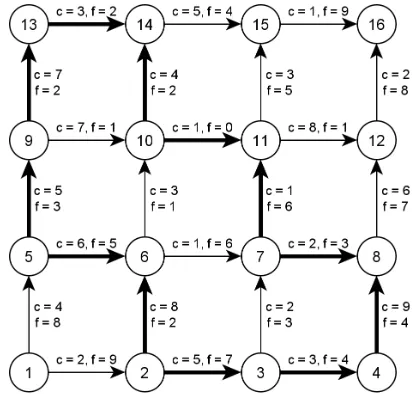
The Traffic Assignment Problem can be seen as an generalized version of the minimum cost flow problem. A technique widely used in algorithms for the min-imum cost flow problem is identifying negative cost cycles and reducing flow on these negative cost cycles. Examples of these algorithms are described by Klein [20] and Goldberg and Tarjan [21]. A negative cost cycle is a sequence of nodes

C ={n1, n2, . . . , nx} such that n1 =nx and every two consecutive nodes are

con-nected by either a link in the same direction as the cycle, called a forward link (ni, ni+1)∈Aor a link in the direction opposite to the direction of the cycle, called a backward link (ni+1, ni)∈A. The set of forward links of a cycle is calledF, the

set of backward links is calledB. Also each backward link in a negative cost cycle should have positive flow and the sum of the link costs of the negative cycle cC,

wherecC =P_a∈Fca−

P

a∈Bca, should be negative. If we defineδ = mina∈Bfa, we

can addδ units of flow to each forward link and subtractδ units of flow from each backward link. This operation is called sending δ units of flow along the cycle. It leaves all flow constraints satisfied and reduces the overall cost of the flow, because

cC is negative. An example of a negative cost cycle is given in figure 3.1 by the

clockwise path through the links in bold. Here δ = mina∈Bfa = f(10,14) = 2 and

cC =−2. Sending an amount of less than 2 units of flow along the cycle keeps all

flows positive and results in a reduction of the total cost.

In TAPAS flows are saved for each origin separately. Given a flow pattern f = (fpa, p∈No, a∈A) that is not converged for at least one originp, TAPAS improves

the solution by searching the sub graph Gp of all links that carry flow coming

from origin p for two types of negative cost cycles. The first and simplest one is a cycle C that consists only of backward links. In this case there is cyclic flow present on the network for origin p. A UE solution can not contain cyclic flow, so we can take δp = mina∈Cfpa and eliminate the cycle by sending δp units of

(20)

[image:20.596.175.381.85.282.2]

Figure 3.1: Example of a negative cost cycle

flow along it. Finding such a cycle can be done efficiently by algorithms such as Tarjan’s algorithm described in [22] or the path-based strong component algorithm by Dijkstra [23, Ch. 25]. The second type of negative cost cycle is a Pair of Alternative Segments: two route segments that have the same diverge node and merge node, and no other nodes in common, where the segment with the highest cost has positive flow on each link of the segment. If we choose the direction of the negative cost cycle such that all links in the lower cost segment are forward links and all links in the higher cost segment are backward links, we can shift flow from the high cost segment to the lower cost alternative by sending flow along the cycle. This results in a decrease of the objective function. The basic steps of the algorithm are therefore identifying and removing cyclic OB flow, identifying PASs and shifting OB flow from the high cost segment to the low cost alternative for all PASs.

TAPAS shares similarities with the bush-based algorithm Algorithm B, introduced by Dial [8]. Both use solution variables fpa that are disaggregated by origin and

also flow shifts are performed by shifting flow from a high cost route segment to a low cost alternative. There are also differences: Algorithm B stores an acyclic set of links called a bushBp for each origin p. Flow is shifted only between links that

are part of the bush. So the main steps of Algorithm B are adding all links that are part of the shortest path tree of each origin p to the bushes Bp and equilibriating

(21)

[image:21.596.176.452.84.307.2]

Chapter 3. A Detailed Description of TAPAS 17

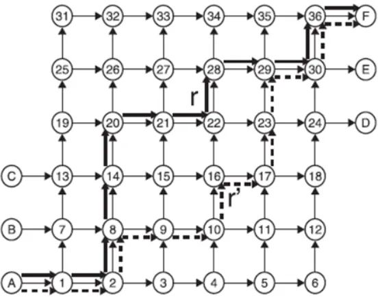
Figure 3.2: Example of a PAS

does not need to store all bushes. TAPAS uses a different approach and stores all PASs that are found, so that the algorithm can prevent constructing the same PAS over and over again. Moreover, TAPAS stores all relevant origins for a PAS. This way flow shifts can be performed on path segments that are used by several origins in one calculation.

We can show the strength and flexibility of the PAS structure using the example of page 1028 of Bar-Gera [3] using the network shown in figure 3.2. Here two routes,

(22)

PASs in a specific order, as shown in table 3.1. Moreover, a basic PAS such as

{[14,20,21],[14,15,21]} can also be used for routes between all other OD pairs in the example. Therefore, the set of 25 basic PASs can be used to perform flow shifts between any two routes for all nine OD pairs.

As seen in the example it is possible to perform flow shifts between any two routes in the network using only a small set of PASs. Such a set is called a covering set. When all PASs in the covering set that have flow on both segments have segments of equal cost, all pairs of routes using any combination of these PASs have the same cost and UE is reached. In theory any covering PAS set can be used to reach equilibrium, but in practice some PASs move flow much more efficient than others. Therefore in each iteration the algorithm will evaluate the effectiveness of PASs, which will be covered in detail in section 3.3. So the main iteration scheme of the algorithm can be divided into two main parts: updating the PAS list by adding new PASs that lead to an improvement on the current solution and removing outdated or inefficient PASs, and shifting flow between the segments of the PASs to reduce the objective function. An overview of the general structure of TAPAS as presented in [3] is given in algorithm 1, with references to sections containing more information on each topic in parentheses.

The rest of this chapter is built up as follows: section 3.1 treats PAS removal and PAS construction, section 3.2 describes flow shifts, in section 3.3 conditions for effective PASs are treated. Section 3.4 describes branch shifts, which are needed when no effective new PAS can be found for a certain link. Section 3.5 describes the cyclic flow removal procedure. In section 3.6 the property of proportionality is explained and a method for calculating proportionality is described. Finally section 3.7 gives a formal proof for the convergence of the algorithm.

Used PAS Resulting route

A,1,2,8,14,20,21,22,28,29,30,36, F (route r)

{[14,20,21],[14,15,20]} A,1,2,8,14,15,21,22,28,29,30,36, F

{[15,21,22],[15,16,22]} A,1,2,8,14,15,16,22,28,29,30,36, F

{[8,14,15],[8,9,15]} A,1,2,8,9,15,16,22,28,29,30,36, F

{[9,15,16],[9,10,16]} A,1,2,8,9,10,16,22,28,29,30,36, F

{[22,28,29],[22,23,29]} A,1,2,8,9,10,16,22,23,29,30,36, F

[image:22.596.82.481.551.669.2]

{[16,22,23],[16,17,23]} A,1,2,8,9,10,16,17,23,29,30,36, F (route r0)

(23)

Algorithm 1: Overview of TAPAS

Find an initial solution using an AON assignment Define maximum allowed duality gap

Set iteration counteri= 1

Define maximum amount of iterations is

while Duality gap> and i <=is do

for each PAS P do Remove if needed(3.1) Check for effectiveness(3.3) end

for each origin p do

Construct the Shortest Path Tree SP Tp for originp using current flow

solution

for each link a where fpa >0 and a /∈SP Tp do

Construct new PAS or add pas relevant origin to an existing PAS (3.1)

end end

for each effective PAS do

Shift flow for all relevant origins (3.2) end

Remove cyclic flow(3.5)

Perform proportionality iteration (3.6) Calculate new duality gap

i+ + end

while not proportionalized do

Perform proportionality iteration (3.6) end

3.1 PAS Construction

Updating the PAS set consists of three operations:

• remove unused PASs

• check PASs for cost and flow effectiveness (treated in section 3.3)

• constructing new PASs where needed

(24)

effectiveness checks. In the current implementation a PAS is removed if it has not been used in the last three main iterations.

For PAS construction we first need to introduce the notion of reduced cost. The reduced cost rcpa is defined for each origin link combination (p, a) as:

rcpa =πpat+ca(f)−πpah

Hereπpah is the cost of the shortest route from originp to nodeah when using all

links is allowed,πpat+ca(f) is the cost of the shortest path from ptoah provided

that link a is the last link of the path. The reduced cost can be interpreted as the penalty in travel cost that is charged for using link a to reach node ah. The

reduced cost is always non-negative and is only equal to zero when link a is part of the shortest path fromp to ah. In each iteration the algorithm checks for each

origin p if PASs are needed. First the shortest path tree (SPT) from p to each noden is calculated using Dijkstra’s algorithm. In a UE solution each link a that carries flow from originphas reduced costrcpa = 0, so a PAS is needed when there

is a linka that carries flow originating from origin p, but where rcpa>0. We call

such a link a a critical link. The logical candidate of the low cost segment is (a part of) the current shortest path fromp toah. The last link of the shortest path

from pto ah is called the shortest path alternative a0 of critical link a. Therefore

we visit all links to check if link a ending at node n has positive OB flow from origin p and has rcpa >0. We can achieve an improved solution by shifting flow

from the critical linka to the shortest path alternative linka0 also ending at node

ah. Node ah will be the end node of the segments for the PAS, called the merge

node. We construct a new PAS by backtracking from at over the links that carry

OB flow from origin p using a breadth first search until a node is found that is part of the shortest path from p to ah. We use a breadth first search to ensure

that the segments will be as short as possible. At some point in the breadth first search we will meet a node m that is in the shortest path from p toah. This will

be the begin node of the segments for the PAS, called the diverge node. Segment

s1 will consist of the links traversed in the backtracking search from node ah via

link a to node m, segment s2 will consist of all links connecting node m to node

ah in the SPT.

(25)

[image:25.596.195.442.81.243.2]

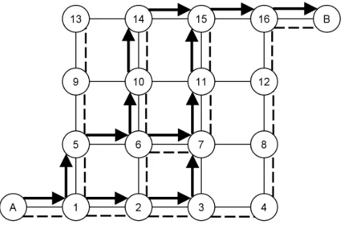
Figure 3.3: PAS Identification

node 6 over the flow carrying links until it meets a node that is part of the shortest path from A to 6. In this case there is only one possible route us-ing the flow carryus-ing links and the backtrackus-ing search will meet the shortest path at node 1, resulting in the PAS {[1,5,6],[1,2,6]}. Similarly, the critical link (14,15) will lead to the PAS {[6,10,14,15],[6,7,11,15]}. The advantage of using a breadth first search will be demonstrated by critical link (15,16). A naive backtracking procedure may result in a needlessly long PAS such as

{[1,5,6,7,11,15,16],[1,2,3,4,8,12,16]}. The breadth first search visits the flow carrying links in the order (14,15), (11,15), (10,14), (7,11), (6,10), (6,7), (3,7). At this point a link contained in the shortest path from the origin to the merge node is found, resulting in the PAS{[3,7,11,15,16],[3,4,8,12,16]}.

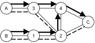
On page 1030 of the original paper [3] the procedure for adding an origin as relevant to an existing PAS is described as follows. When a critical link a and its shortest path alternativea0 are found, the algorithm searches the PAS list for PASs whose segments end with links a and a0. If such a PAS is found, the origin is added as relevant. This method is incomplete, as can be seen in figure 3.4. There is a positive flow on paths [A,3,4, C] and [B,1,2,4, C] and the shortest paths are again given by the dashed lines. Let’s assume that there currently is one PAS

(26)

[image:26.596.200.362.81.154.2]

Figure 3.4: Origin incorrectly denoted as relevant

If there exists a PAS that satisfies these requirements, we can add pas a relevant origin to the PAS.

3.2 Flow Shifts

Flow shifts between segments of PASs are the easiest part of the algorithm. Only effective PASs are considered for flow shifts, so that the algorithm does not spend any time on ineffective flow shifts. For a flow shift on PAS P with segments s1 and s2 we first need to set segments1 as the segment with the highest cost. Then for each relevant origin p ∈ OP we determine the maximal flow fp∗ that can be

shifted, so that all OB flows remain nonnegative:

f_p∗ = min

a∈s1

fpa

The total amount of flow that can be shifted is:

fmax =

X

p∈OP

f_p∗

If the maximum allowed amount of flow is shifted, we would get a new link flow solutionf0:

f_a0 =         

fa−fmax a⊆s1

fa+fmax a⊆s2

fa otherwise

If shifting all allowed flow still leaves segments2 as shortest segment we can simply shift all allowed flow. Otherwise, we determine the optimal step size 0≤λ≤1 by performing a line search. We solve the problem

min 0≤λ≤1

X

a∈A

Z (1−λ)fa+λfa0

0

(27)

Flows on links that are not part of one of the segments of the PAS do not change, so solving equation 3.2.1 is equivalent to solving

min 0≤λ≤1

X

a∈s1

Z fa−λfmax

0

ca(ω) dω+

X

a∈s2

Z fa+λfmax

0

ca(ω) dω (3.2.2)

This problem can be solved by taking the derivative and finding the root using for instance Newton’s method. The last step is to update OB flows and link costs:

fpa =fpa−λfp∗ ∀a∈s1

fpa =fpa+λfp∗ ∀a∈s2

Empirical evidence shows that the PAS searching procedure takes much more time than the flow shifting procedure. Also, in later iterations when the PAS set is al-most completely covering and the search for new PASs only introduces a few new PASs, it would be wise to spend more time on flow shifts. Bar-Gera proposes an inner loop for the flow shifts, as can be seen in the general structure of TAPAS in algorithm 1. Bar-Gera uses 20 flow shift inner loops per iteration in his imple-mentation. Our prototype uses a slightly different approach: less time is spent on flow shifts in early iterations, when the solution is far from being equilibriated. A substantial amount of flow that is shifted during the early iterations will be shifted away from the segments of the existing PASs when new ones are found in later iterations. Therefore the number of inner loops is chosen to be min(i,20), where i is the number of iterations, so that the amount of flow shifts is increased gradually.

3.3 Cost and Flow Effectiveness of PASs

(28)

A PAS is cost effective for origin p if the cost difference between the segments is large enough. To assess this formally, we again need the reduced cost for the last link a of segment s1 of the PAS, with ah as the merge node of the PAS. As a

reminder, the reduced cost rcpa is defined for each origin link combination as:

rcpa =πpat+ca(f)−πpah

The reduced cost can be seen as the minimal improvement in travel time that could be made by a traveler if the traveler stops using the current route that approaches node ah using link a and instead uses the shortest path from p to ah. If a PAS

with link a as the last link of the high cost segment has a cost difference that is smaller than a factor µ = 0.5 of the reduced cost, then both segments will have equal cost when only a small fraction of the maximum allowed flow is shifted. This is a problem especially when the PAS is part of a sequence of PASs that is used to shift flow from one path to another. In this case a lot of iterations are needed to shift large amounts of flow from one path to the other as can be seen in the example below. The PAS is considered not cost effective and a new PAS has to be found with a more efficient low cost segment. Formally, a PAS, given by s1 and

s2, with segment s1 as high cost segment and link aas last link of s1 is considered cost effective for origin pif

cs1 −cs2 ≥µ·rcpa

For the flow effectiveness of a PAS for origin p we look at the amount of flow fpa

on the last linkaof segment s1. We want to be able to shift all or most of the flow from segment s1 to segment s2. However, the nonnegativity constraints restrict the maximal flow shift for origin p to the minimal flow f_p∗ = mina∈s1fpa on s1. If

f_p∗ is small, we can only shift a very small amount of flow. If this PAS is part of a chain, we get a so called cascading effect, as can be seen in the example below. To counter this phenomenon, we define a PAS to be flow effective if the ratio between the minimal flow f_p∗ and the flow fpa on the last link ofs1 is greater than a factor

ν = 0.25. We formally define a PAS with segment s1 as high cost segment and link a as last link ofs1 to be flow effective for origin pif

f_p∗ ≥ν·fpa

If a PAS is not flow effective, we have to find a new PAS that uses another high cost segment.

(29)

[image:29.596.230.400.82.246.2]

Figure 3.5: Example of ineffective PASs

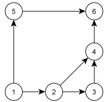
with the network shown in figure 3.5 where flow is sent from origin 1 to des-tination 6. There are three possible PASs: P1 = {[1,5,6],[1,2,3,4,6]}, P2 =

{[1,5,6],[1,2,4,6]} and P3 = {[2,3,4],[2,4]}. Any two of these PASs forms a covering PAS set and be used to perform all flow shifts between routes in this network. Assume that PASP2 and P3 are used and links have the following costs:

c(1,5) =c(5,6) = 2, c(1,2) =c(4,5) = 1, c(2,3) =c(3,4) = 0.5 andc(2,4) = (2−m) +f(2,4) wheremis an arbitrary number between 0 and 1. Also assume that there is a flow of 1 on route [1,5,6], the flow is zero everywhere else. In the flow shift procedure first PAS P2 is used to shift m units of flow from segment [1,5,6] to [1,2,4,6]. Now both segments have equal costs and PAS P3 can be used to shift m units of flow to segment [2,3,4]. This sequence will be repeated until all flow is shifted to route [1,2,3,4,6]. When m is chosen close to 0, this procedure could in theory take infinitely many iterations. In this case PAS P2 is not cost effective, because the reduced cost of link (5,6) is 1, and cs1−cs2 =m ≤ µ·1. The algorithm will stop using PAS 2 and add PAS 1 which will find the UE solution in one flow shift. Now we change link costs to 1 for all links except link (2,4), which will have cost

c(2,4) = (2−m)+f(2,4). There is a flow of 1 on path [1,2,3,4,6] and zero everywhere else. Even though both PASs are cost effective we get a similar behavior: first PAS

P3 is used to shiftmunits of flow to segment [2,4] and then PASP2 is only allowed to shift a maximum of m units of flow to segment [1,5,6], because otherwise the non-negativity constraints are violated. The sequence is then repeated until all flow is shifted. This process can take arbitrarily long if we choosemsmall enough. PAS P2 is not flow effective and the algorithm will use PASP1 instead.

(30)

[image:30.596.159.403.83.243.2]

Figure 3.6: Example of a branch

PAS is declared effective. Flow shifts are then performed on all relevant origins. In the second method effectiveness is determined separately for each relevant origin. Using this method flow shifts are only performed on the relevant origins that are both cost and flow effective. If a relevant origin fails to satisfy one or both of the requirements the PAS is declared not effective for that relevant origin and a new PAS has to be found for the origin. In the original paper this issue is not addressed, but in our prototype we choose to use the second method. This is because in the first method a PAS may not meet both effectiveness requirements for some relevant origins, while it may still be considered effective because there is another relevant origin that does meet both requirements. This can severely slow down convergence for the noneffective relevant origins, as shown in the example in figure 3.5. In such a case we are better of searching a new PAS for these origins.

3.4 Branch Shift

For a new PAS for originpwith critical linka it always holds thatcs1−cs2 ≥rcpa,

so any new PAS generated by the algorithm is always cost effective. This may not be the case for flow effectiveness. New PASs are checked for flow effectiveness and if a new PAS is not flow effective, the breadth first search will continue until another diverge node is found. In later iterations, when flow is highly spread out, there is a possibility that no flow effective PAS exists for critical linka. This is a scenario that is likely to happen, since TAPAS attempts to maintain a proportionalized flow solution (described in section 3.6). In this case a new mechanic called a branch shift is performed. Unlike a flow shift where flow is shifted from one route segment to another, in a branch shift flow is shifted from all route segments from

(31)

of a route segment from an origin p to the merge node ah that carries flow from

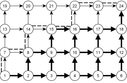
p and that has the critical link a as last link is called a branch. An example of a branch is shown in figure 3.6. Here the critical link is link (18,24). The least cost route from origin 1 to node 24 is represented by the dashed line. All links that are part of any flow carrying route segment that ends with the critical link are in bold. Note that this is not necessary all flow to node 24; there may be flow that enters node 24 through link (23,24). No description of the calculation of a branch shift is given in [3], so an original method is stated here. We useS to denote the set of all flow carrying route segments that start at pand enter ah through a. In

a branch shift flow is shifted from all route segments in S. The maximal allowed flow shift is the OB flow on the critical link: f_p∗ =fpa. Using the segment flows for

each route segments inS, we can calculate the proportion prpa0 of f∗

p that passes

through each linka0 in the branch. We call this proportion the branch proportion of link a0. We can calculate prpa0 by dividing the sum of the segment flows on all

segments in S that contain a0 by the max flow shift. The flow on each segment s

inS can be calculated using

kps =

Y

b∈s

αpb

!

·f_p∗

So the proportion of branch flow that is on link a0 is

prpa0 =

P

(s∈S|a0_∈_s₎kps

f∗

p

(3.4.1)

= P

(s∈S|a0_∈_s₎

Q

b∈sαpb

·f_p∗ f∗

p

(3.4.2)

= X

(s∈S|a0_∈_s₎

Y

b∈s

αpb (3.4.3)

This formula requires that all possible path segments in the branch are calculated. Alternatively, we can calculate the branch proportion recursively by setting the branch proportion topra = 1 for the critical link and toprb = 0 for all linksb that

are not part of the branch. We can then traverse backward through the branch using

prpa0 =α_pa0 ·

X

asuc∈OU T_a0

h

(32)

This way we only need to visit each link once. We can then calculate the optimal step sizeλ using

min 0≤λ≤1

X

a∈A

Z fpa+δa,sptλfp∗−δa,bλprafp∗

0

c(ω)dω

where δa,spt is 1 if a is part of the shortest path segment and 0 otherwise, δa,b is 1

if a is part of the branch and 0 otherwise. The flow update is performed using

fpa0_,new =f_pa0+δ_a0_,sptλf∗

p −δa0_,bλ pr_a0f∗

p

3.5 Cyclic Flow Removal

Cyclic flow can be generated in the network due to the structure of PAS flow shifts. This flow has to be eliminated from the network, because UE can not be achieved when there is cyclic flow present on the network. Several algorithms that identify cycles in networks exist. The most efficient of these algorithms is Tarjan’s strongly connected components algorithm, which has to be altered slightly in order to be able to identify cycles instead of connected component. A connected component is a set of nodes N0 ⊆ N such that each node n ∈ N0 can be reached by all other nodes {n0 ∈ N0|n0 6= n}. A connected component can contain multiple cycles and some edges can be included in more than on cycle. Pseudocode for the adapted version of Tarjan’s algorithm can be found in appendix B. This cyclic flow removal algorithm differs from Tarjan’s algorithm in that this version visits links instead of nodes. Another difference is that instead of finding a complete connected component, this algorithm stops searching when a cycle is found and removes cyclic flow immediately. After removing the cyclic flow all links in the cycle are flagged as unvisited so that the procedure can visit these links again in case they are part of more cycles. The procedure resumes the search for cycles at the link of the cycle it first encountered. If a flow cycle C = [a1, a2, . . . , ai] is

found for origin p, we determine the total flow to be removed

fmax = min

a∈C fpa (3.5.1)

The OB flows will be updated using

fpa,new =fpa−fmax (3.5.2)

(33)

[image:33.596.189.438.83.186.2]

Figure 3.7: Proportionality example

3.6 Proportionality

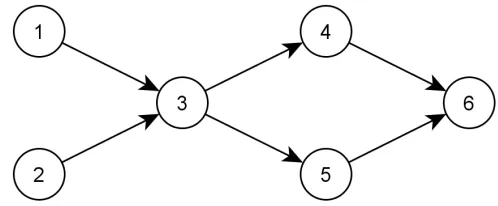
While the User Equilibrium conditions guarantee a unique optimal solution of Beckmanns problem (BE) in terms of link flows, this is not the case for route flows (see remark r1 in section 2.3). When there are OD pairs that have a common pair of flow carrying segments, there are infinitely many route flow solutions, as can be seen in the example in figure 3.7. Here the flow demand is 1 for OD pairs (1,6) and (2,6) and each link carries one unit of flow in the UE solution. Each OD pair has two UE routes that have a common pair of segmentss1 = [3,4,6] and

s2 = [3,5,6]. Now any feasible OB flow that has segment flows k1,s1 = 1−k2,s1

andk1,s2 = 1−k2,s2 is a UE solution. TAPAS tries to find a realistic route solution

h by introducing two properties for route flow solutions: route consistency and route proportionality. A UE solution is called consistent if for all OD pairs {p, q}

all UE routes, i.e. all routes rbetweenpandq withfa>0∀a∈r, have route flow

hr >0. This condition is a natural extention to the User Equilibrium principles:

users are indifferent between UE routes, so all of these routes are used by some portion of the flow. For the proportionality condition we first introduce the notion of alternative routes. Let r1 be a route from originp1 to destination q1 and let r2 be a route from p2 to q2. Assume PAS P with segments s1, s2 has equal cost for both segments and let node d and m be the diverge node and merge node of the segments of P. The origin based proportion of a PAS is defined as

ρp,s1 =

kp,s1

kp,s1 +kp,s2

Routes r1 and r2 are called a pair of alternative routes if they consist of the following route segments:

r1 = [rp1,d, s1, rm,q1]

(34)

Here rp1,d is the route segment from p1 to the diverge node of PAS P and rm,q1

is the route segment from the merge node of PAS P to q1. We define the route proportion ρr1,r2 as

ρr1,r2 =ρp,s1

We call a UE solution proportional if for any two pairs of alternative routes (r1, r2), (r3, r4) that use PAS P, with routes r1 and r3 using segments1 and routesr2 and

r4 using segment s2, we have that ρ(r1, r2) =ρ(r3, r4).

Finding a completely consistent UE solution is difficult, but TAPAS tries to satisfy the consistency condition by adding many relevant origins to a PAS. This way, each relevant origin will carry flow on both segments of the PAS by the proportionality condition. It is well-known that for given UE (f∗,h) with uniquely determined link flowf∗ the corresponding pathflowhsatisfies consistency and the proportionality conditions if (for given f∗) the part h is a maximizer of the following entropy maximization problem (see Larsson et al. [24]):

max E(h) =−X r∈R

hr·log

hr

dpq

s.t. X

r∈Rpq

hr =dpq ∀p∈No, q ∈Nd(p)

X

r∈R:a⊆r

hr =fa∗ ∀a∈A

h≥0

TAPAS solves the proportionality problem approximately on PAS level by itera-tively applying a flow shift between the relevant origins of a PAS that keeps the total link flows identical and maximizes entropy for the PAS, as described in Bar-Gera [3]. We want to find the vector of origin-based PAS adjustments ∆fpa such

that

∆fpa=

        

δp a ⊆s1

(35)

We can find ∆fpa by calculating the solution to the maximum entropy problem

for a single PAS. Here f is the vector of the OB flows fpa:

max E(f + ∆f) =− X p∈No

X

a∈A

(fpa+ ∆fpa)·log

fpa+ ∆fpa

gpah(f + ∆f)

s.t. X

p

δp = 0

f + ∆f ≥0

Here the first constraint ensures that the total link flow on each link does not change. The second constraint ensures that all OB flows remain nonnegative. The Lagrangian for this problem is

maxL=E(f + ∆f(δ)) +λ·

X p δp (3.6.1)

s.t. f + ∆f(δ)≥0 (3.6.2)

To find the derivative of equation 3.6.1 with respect to δp we look at each origin

link combination separately:

Epa(f + ∆f(δ)) =−(fpa+ ∆fpa(δ))·log

fpa+ ∆fpa(δ)

gpah(f + ∆f(δ))

(3.6.3)

E(f + ∆f(δ)) = X

p∈No

X

a∈A

Epa(f + ∆f(δ)) (3.6.4)

First we look at the derivative of the last links of the segmentsa1 ⊆s1 anda2 ⊆s2, with merge noden =a1h =a2h. Here we have that gpn(f+ ∆f(δ)) = gpn, because

the adjustment ons1 cancels out the adjustment on s2. So we get

∂Epa1

∂δp

=−log

fpa1 +δp

gpn

−1

∂Epa2

∂δp

= log

fpa2 +δp

gpn

+ 1

All other OB flows on links that haven as head node are unchanged, so the total contribution to the derivative of links that end at the merge node is

X

a|ah=n

∂Epa

∂δp

=−log

fpa1 +δp

gpn

+ log

fpa2 −δp

gpn

(3.6.5)

For other links a0|a0_h =j =6 n in s1 the change in origin based link flow fpa0 and in

(36)

link combination pa0 is

∂Epa0

∂δp

=−log

fpa0+δ_p

gpj+δp

−1 + fpa0 +δp

gpj+δp

(3.6.6)

All other linksa00 that end at nodej also contribute to the derivative, because the node flow gpj is changed. The contribution of these links is

∂Epa00

∂δp

= fpa00

gpj+δp

(3.6.7)

Adding equations 3.6.6 and 3.6.7 together gives the total contribution of links ending at j:

X

a|ah=j

∂Epa

∂δp

=−log

fpa0 +δ_p

gpj+δp

(3.6.8)

Along the same line we can get the contribution to the derivative of a linka0 ⊆s2 and all other links that end at node a0_h =j 6=n

X

a|ah=j

∂Epa

∂δp

=−log

fpa0 −δ_p

gpj−δp

(3.6.9)

We can get the total entropy derivative by adding the derivative components of each node in the PAS using equations 3.6.5, 3.6.8 and 3.6.9:

∂E ∂δp

=−X a⊆s1

log

fpa+δp

gpah(δp)

+X

a⊆s2

log

fpa−δp

gpah(δp)

=−log

kps1(δ)

gps1h(δ)

+ log

kps2(δ)

gps2h(δ)

=−log

kps1(δ)

kps2(δ)

Herekps(δ) is the flow on segments from origin pgiven the adjustment δ. So the

optimality conditions of 3.6.1 are:

∂L

∂δp

=−log kps1(δp)

kps2(δp)

+λ= 0

kps1(δp)

kps2(δp)

= exp(λ) An equivalent system for the unknowns δp, λ is

ρp(δp) :=

kps1(δp)

kps1(δp) +kps2(δp)

(37)

In [3] Bar-Gera proposes a method for solving this system of KKT-conditions for

δp, λ subject to the constraint f + ∆(f)≥0.

3.7 Proof of Convergence

This section gives a formal proof of convergence for TAPAS. This proof is along the lines of the proof given by Bar-Gera in section 6.4 of [3], but is worked out in greater detail. For this proof we use a simplified version of TAPAS, shown in algorithm 2, where in each iteration only critical origin-link combinations (p, a) that have ξ(fpa, rcpa) > are considered. This is halved after each iteration

and the algorithm stops if becomes smaller than a given s. For each critical

origin-link combination either a flow shift or a branch shift is performed. This algorithm is different from the normal version of TAPAS, but it is easier to prove convergence for. Equilibrium is reached if reaches 0, i.e. if there are no more critical origin-link combinations. In this case, for each origin p and for all flow carrying linksathe reduced cost rcpa = 0, so all flow carrying links are part of the

shortest path tree of p. We show that we can find a lower bound on the reduction of the objective function for flow shifts and branch shifts for the critical link. For the proof we assume that the cost functions ca(f) are Lipschitz continuous with

Lipschitz constant L:

|ca(f +δ)−ca(f)| ≤ Lδ ∀a, feasible f (3.7.1)

This is not a strong condition, because demands are finite. Furthermore we use the objective function z(f) given in equation 2.3.5, the effectiveness definitions given in section 3.3, the reduced cost defined in section 3.1 and ξ(fpa, rcpa), which

is defined as

ξ(fpa, rcpa) := min

_µ2_rc2

pa(f)

8L|A| ,

µν

2 fparcpa(f)

(3.7.2)

First we prove that a flow shift on an efficient PAS reduces the objective function by at least ξ(fpa, rcpa).

(38)

Algorithm 2: Simplified version of TAPAS used for convergence proof

Initialize: set =0,s 0, find a feasible flow f0, set µand ν as described in 3.3

Set k = 0

while ≥s do

while for fk, ∃a, p such that ξ(fk

pa, rcpa)≥ do

if ∃ an efficient PASP for p and a then Perform a flow shift for P

end else

Perform a branch shift forp and a

end

k+ +

Set fk as the new flow vector end

=/2 end

Proof. Letδ >0 be the amount of flow shifted on the PAS. Then

f_pa0 =fpa−δ ∀a∈s1

f_pa0 =fpa+δ ∀a∈s2

f_pa0 =fpa ∀a∈A\(s1∪s2)

We have that

− L|δ| ≤ca(f+δ)−ca(f)≤ L|δ| ∀a, f (3.7.3)

By the mean value theorem we get that for each linka ∈s1for some ˜fa∈(fa−δ, fa)

Z fa

fa−δ

ca(ω)dω =ca( ˜fa)δ (3.7.4) ≥δ(ca(fa)− L|f˜a−fa|) (3.7.5) ≥δ(ca(fa)− Lδ) (3.7.6)

and similarly for each link b∈s2 Z fb+δ

fb

(39)

So the difference in the objective function is, using 3.7.6 and 3.7.9

∆ :=z(f)−z(f0) = zs1(f) +zs2(f)−zs1(f 0

)−zs2(f 0

) (3.7.10) = X

a∈s1

Z fa

fa−δ

ca(ω)dω−

X

b∈s1

Z fb+δ

fb

cb(ω)dω (3.7.11) ≥δ(cs1(f)−cs2(f)−2|A|δL) (3.7.12)

≥δ(µrcpa(f)−2|A|δL) (3.7.13)

Here the last inequality is due to the fact that the PAS is cost effective. Now define

δ∗ := 1 2

µ rcpa(f)

2|A|L (3.7.14)

We can choose our flow shift δ = min{δ∗, f_p∗}, where f_p∗ = minb∈s1fpa. Here we

have that f_p∗ ≥νfpa, due to the fact that the PAS is flow effective. If δ∗ ≤νfpa, a

flow shift of δ∗ is feasible and yields ∆≥δ∗1

2µ rcpa(f) =

µ2_rc2

pa(f)

8|A|L (3.7.15)

Otherwise we can shift νfpa amounts of flow, yielding

∆≥νfpa

µ rcpa(f)

2 (3.7.16)

We will now show that a similar reduction in objective function can be achieved by a branch shift.

Lemma 3.2. The reduction ∆ in the objective function z of a branch shift is

∆≥min

fpa

rcpa(f)

2 ,

rc2

pa(f)

8|A|L

(3.7.17)

Proof. Let a be a critical link for p with respect to flow f and Bp be the branch

spanned by all segmentss1, .., sk frompto ah through a. Supposes2 is a shortest path segment from p toah. By definition we have for all si

c_si(f)−c_s

2(f)≥rcpa(f) (3.7.18)

Let

f_p∗(i) := min

b∈si

(40)

Now since all flow fpa comes via one of the segments s1, .., sk inBp we have that k

X

i=1

f_p∗(i)≥fpa (3.7.20)

So we can choose flowsf_pi for each segment inB such thatf_pi ≤f_p∗(i) andP

if i p =

fpa. Now consider simultaneous flow shifts δi from si to s2 denoted by f → f

0

. We define δ = P

iδi. By the analysis used in the proof of lemma 3.1 and using

equation 3.7.18 we find the difference in objective function values

∆ := z(f)−z(f0) (3.7.21) =X

i

X

a∈si

Z fa

fa−δi

ca(ω)dω−

X

b∈s2

Z fb+δ

fb

cb(ω)dω (3.7.22)

≥X

i

δi(csi(f)− |A|Lδ_i)−δ(c_s₂(f) +|A|Lδ) (3.7.23)

=X

i

δi[(csi(f)−c_s₂(f))−2|A|Lδ] (3.7.24)

≥X

i

δi(rcpa(f)−2|A|Lδ) (3.7.25)

In order to satisfy nonnegativity constraints, we can choose flow shiftsδi such that

δi ≤fpi, δ ≤δ

∗

:= 1 2

rcpa(f)

2|A|L (3.7.26)

In case P

if i

p ≥δ∗ we can chooseδi ≤fpi such that

P

iδi =δ

∗ _{and we can shift} _δ

i

fromsi tos2 to obtain

∆≥ k

X

i=1

δi

rcpa(f)

2 (3.7.27)

=δ∗rcpa(f)

2 (3.7.28)

= rcpa(f)

8|A|L (3.7.29)

In case P

ifpi ≤δ

∗ _{we can choose} _δ

i =fpi and perform this shift to obtain

∆≥ k

X

i=1

f_pircpa(f)

2 (3.7.30)

=fpa

rcpa(f)

(41)

Now we arrive at the convergence theorem, which follows from lemmas 3.1 and 3.2.

Theorem 3.3. Let s = 0, let fk be the sequence of feasible flows generated by

algorithm 2 and let z(fk) be the sequence of objective functions induced by fk. Then the sequence z(fk) converges to the minimum value of Beckmann’s program (BE). Moreover the sequence fk has a (at least one) limit point f∗. Each such limit point f∗ is a UE.

Proof. Since the sequence z(fk) is monotonically decreasing we only have to show that f∗ is a UE. Suppose that f∗ is not a UE. Then the value ξ(f_pa∗ , rcpa(f∗)) :=

σ >0. But then according to algorithm 2 in each step k of this algorithm we have

ξ(fk

pa, rcpa(f∗)) ≥ δ/2 and by lemma 3.1 and 3.2 in each step the value of z(fk)

(42)

(43)

Chapter 4 Traffic Assignment Problem with

Asymmetric Costs

Introducing asymmetric cost functions to TAP makes the problem much more difficult to solve efficiently, as shown in section 2.4. This chapter describes how OmniTRANS deals with junction modeling and proposes several methods that can be added to TAPAS in order to be able to handle asymmetric cost functions. Section 4.1 explains how junction modeling is treated in OmniTRANS and shows the mathematical difficulties that arise from asymmetrical cost functions. Section 4.2 describes the changes that need to be made to incorporate junction modeling in TAPAS. In section 4.3 some heuristics for finding a descent direction using the asymmetric cost functions are treated.

4.1 Junction Modelling in OmniTRANS

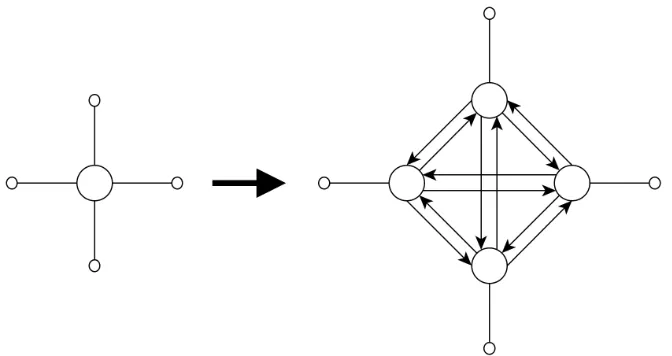
In OmniTRANS junction delays are modeled by expanding each junction node as can be seen in figure 4.1. Each arm of the junction is represented by a node and for each possible turn a link between two arms is added, called a turn. Since OmniTRANS supports both three way junctions and four way junctions, each junction node will be blown up to at most four nodes and twelve links. The links that are added when junction nodes are expanded are called turns. When turns are added we divide the set A in two sets: the set of turns, called At and the

set of regular links, called Al, such that A\ Al = At. OmniTRANS has put

several restictions on paths containing turns: a link entering an junction must be followed by a turn of that junction and this turn has to be followed by an exit link of the junction. Illegal turn movements such as traveling along a turn of a

(44)

[image:44.596.114.450.81.259.2]

Figure 4.1: A junction node being expanded

junction and then immediately traveling along another turn in the same junction are prevented by saving a list of allowed turns for each entry link and for each exit link of the junction and a list of allowed entry links and a list of allowed exit links for each turn. Each turn has a cost function that depends on the type of the turn, the load on the turn itself and conflicting turns and several other user defined parameters such as number of lanes or free flow speed. OmniTRANS supports seven types of junctions: equal junctions, priority junctions with the main road going straight or turning, all stop junctions, signalized junctions and signalized and unsignalized roundabouts. Some examples of capacity and delay functions of junctions in OmniTRANS are given in Appendix A.

The objective function of the Beckmann notation, as described in section 2.3, does not exist anymore if we introduce asymmetric link costs. Therefore most traffic modeling software developers use approximations of the turn functions in order to be able to calculate a reasonable solution. Several of these approximations are described in section 4.3. The current implementation of FW in OmniTRANS uses a very simple and pragmatic approximation of the turn functions for its step size calculation: the integral is omitted and instead the turn cost function is used:

z(f) = X

a∈Al

Z fa

0

ca(ω)dω+

X

a∈At

ca(fa) (4.1.1)

(45)

[image:45.596.237.397.83.245.2]

Chapter 4. TAP with Asymmetric Costs 41

Figure 4.2: Example network with a banned turn

that VA uses predetermined step sizes and as such is not affected by errors in the approximations of turn cost function.

4.2 Adjustments to TAPAS

In this section we cover all adjustments needed for TAPAS to be implemented in OmniTRANS. First some examples are given to show the problems that can arise when the original methods of TAPAS are used. Then a solution is proposed. One of the problems with using TAPAS on a network that uses Junction Modeling is that paths generated by PASs as described by Bar-Gera [3] may contain illegal turn movements. We illustrate this problem using the example in figure 4.2. Here turn [2,4,5] is banned. In this network the demand from node 1 to node 7 is 3 units of flow. Link cost functions are as follows: ca = 2 +fa for a = (1,2) and

a= (2,4), ca= 3 +fa for a= (4,6) anda = (6,7), and ca = 1 + 2fa for all other

links. The UE solution has 1.5 units of flow on each link. Figure 4.2 shows the situation just before the first iteration of TAPAS. The initializing AON assignment is shown as bold arrows, the shortest path from node 1 to 7 after the initialization is shown by the dashed line. There are two critical links, (3,4) and (5,7), leading to two obvious PASs, P1 = {[1,2,4],[1,3,4]} and P2 = {[4,5,7],[4,6,7]}. Both PASs are allowed by the definitions stated in section 3.1, but when we perform a flow shift on PAS P1 we may introduce a new path [1,2,4,5,7] that uses the banned turn. We can prevent this by requiring that the flow on section [1,2,4] does not exceed the flow on section [4,6,7]. But this introduced a new problem when we want to shift flow. Segment [4,6,7] has no flow, so shifting flow on PAS

(46)

[image:46.596.158.403.80.327.2]

Figure 4.3: Example network of fig 4.2 with expanded node

on PASP2 equilibriates both segments of the PAS. Now we can perform the shift on P1. The maximum allowed flow shift is 11₃, which still leaves segment [1,2,4] the short segment. If we shift this flow TAPAS reaches a deadlock, because P2 is equilibriated and flow shifts on P1 are limited by the flow on segment [4,6,7]. We can solve this issue by requiring that nodes that have a banned turn are expanded, so they contain all allowed turns (which have zero cost). This can be seen in figure 4.3. Introducing turns on node 4 has ensured that the flow and the shortest path cross but don’t meet at node 4. Now there is only one critical link (5,7), which leads to the PAS{[1,3,4b,4c,5,7],[1,2,4a,4d,6,7]}that can reach equilibrium in one flow shift. With this approach we can circumvent all problems described above and also any potential problems that could arise in a branch shift.

(47)

[image:47.596.167.464.87.363.2]

(a) (b)

Figure 4.4: Example network that identifies the merge node incorrectly

[1,3,5b,5a,5c,7,8] which includes an illegal turn movement. Similar behavior can occur with selecting a diverge node when the first link of one segment is a link and the first link of the other segment is a turn. Part of this problem is already solved by the way the shortest route generation is implemented in OmniTRANS. OmniTRANS takes a link-based approach to saving shortest paths: for each linka

the cost of the shortest path from the origin to the end nodeah via linkais stored

along with the predecessor of link a with this shortest path. So the shortest path tree in OmniTRANS is not really a tree anymore, because shortest path informa-tion is stored for all links, so nodes are reachable through multiple paths. We take advantage of this link-based approach by changing the backtracking phase of the PAS generation procedure as follows: when link a is visited, instead of checking whether nodeatis part of the shortest path from the origin to the critical link, we

(48)

[image:48.596.162.399.89.315.2]

(a) (b)

Figure 4.5: A network that shows the lost PAS efficiency from introducing

junctions

A disadvantage of TAPAS compared to FW is that TAPAS has higher memory usage due to the OB flows that are stored: FW uses|A|entries to store its link flows and TAPAS needs|A|·|O|. Blowing up junctions increases this problem. A possible solution for this is using a sparse matrix representation for the link flows. Empirical evidence has shown that up to 80 percent of OB flows are zero, so a sparse matrix could be a great improvement in memory usage. Blowing up junctions also gives a problem in the efficiency of PAS construction. In figure 4.5(a) we see a network without junctions where flow goes from origin 1 to destinations 5 and 6. As always, the flow is on bolded lines and the shortest path tree is represented by the dashed lines. Here one PAS {[1,2,4],[1,3,4]} is needed and flow is shifted from paths [1,2,4,5] and [1,2,4,6] to paths [1,3,4,5] and [1,3,4,6] simultaneously. If node 4 is blown up, as can be seen in figure 4.5(b), this advantage is lost. Now two PASs are needed: {[1,2,4a,4c],[1,3,4b,4c]} and {[1,2,4a,4d],[1,3,4b,4d]}. While this behavior does not compromise the ability of TAPAS to converge, more PASs are needed and so more memory is needed and computation time goes up.

4.3 Solutions for Asymmetric Cost Functions

(49)

exist anymore. Subsections 4.3.1 and 4.3.2 cover two heuristics that tackle this problem. Also multiple User Equilibria may exist, which makes comparing solu-tions obtained by making small changes to the network or OD matrix or solusolu-tions generated by different algorithms very difficult. In section 4.3.3 a method is de-scribed that tries to ’push’ the solution to the same equilibrium regardless of the starting state of the network.

4.3.1 Diagonalization

The diagonalization algorithm for asymmetric cost TAP was introduced by Florian and Spiess [18]. The idea behind the algorithm is simple: in the cost function for each link all variables of conflicting junctions are fixed, so the link function only depends on the flow on the link itself. This way the link cost functions become separable and we can use the Beckmann program to find an optimal step size given the fixed costs of conflicting turns. To this end a new cost function is defined for links with asymmetric costs:

˜

c_ai(fa) = ca(f1i−1, f

i−1 2 , . . . , f

i−1

a−1, fa, fai+1−1, . . .) (4.3.1) Here i is the iteration number and f_bi−1 is the flow on link b at the end of the iteration i−1. In each iteration the UE is approximated by the problem with the diagonalized turn costs ˜ci

a(fa). Then the cost functions are updated, leading to

improved approximations of the cost functions. This is repeated until fi a = fi

−1

a

for alla∈At. Algorithm 3 shows an overview of the diagonalization algorithm. An

alternative approach, called the streamlined diagonalization algorithm was given by Sheffi [25]. Here only one inner iteration of the used assignment algorithm is performed between consecutive updates of diagonalized cost functions. This method saves a lot of calculation time in early iterations, because the difference betweenf i−1

a andfai is still large, so a lot of time is wasted calculating a converged

solution for the diagonalized turn costs ˜ci a(fa).

A modified version of the streamlined diagonalization algorithm can be used effi-ciently in TAPAS, due to the structure of flow shifts in PASs. Before a flow shift we determine the diagonalized cost function ˜ca(fa) for each turn that is part of

Traffic Assignment with Junction Modeling in TAPAS