Item response theory model with testlet effects: A simulation study investigation of effectiveness in small sample sizes

Item response theory model with testlet effects: A simulation study investigation of effectiveness in small sample sizes

Jeremias Hendrik Marian Wenzel 1st supervisor: Prof. Dr. Ir. Jean-Paul Fox

Abstract

In this article, two different item response theory (IRT) models with testlet effects are compared. Testlets structures account for item interrcorrelations in sets of items, so that conditional

independence for a test can be assumed, even if groups of related items are used in the

testconstruction. The conditional testlet model adds a testlet parameter to the basic IRT model, that models the dependencies among response observations to the same testlet items. The marginal testlet model, by contrast, models them directly as a covariance parameter in the covariance matrix of the distribution of the error. This leads to better parameter estimation for small dependencies. The precision of the parameter estimates under the two models are evaluated for data simulated under the conditional testlet model. The simulation study uses different

Item response theory model with testlet effects: A simulation study investigation of effectiveness in small sample sizes

Introduction

Item response theory is a form of test scoring, which includes the latent ability of a given examinee and the difficulty of the item, in order to estimate the chance of success on a test item. In contrast to classical test theory, which assumes all items to have equal difficulty, the difficulty is estimated per item. This makes it possible to administer test questions in random order. The basic item response theory (IRT) assumes all items to have conditional independence (CI). This means that no items are related to each other given the value of the latent variable. This becomes problematic in the case of so called testlets. Testlets are groups of questions that are inherently related to each other. A common example are multiple questions in a reading comprehension questionnaire. Because it takes some time to read a long section of text, it is useful to ask multiple questions about it. Therefore, all items are pertaining to a single piece of text. It makes intuitive sense that these questions are not independent from each other. Answering correctly on one of them is inherently related to the answering of the others, thus leading to a possible wrong

evaluation of the examinees proficiency. Under the basic IRT model, an examinee who answered three questions correctly from one reading comprehension excerpt would be evaluated equally to a different examinee who answered three individual questions correctly. Their proficiency would be estimated to be the same (given equal difficulty for the items), even though they each showed their knowledge of only one, compared to three pieces of information, respectively. The term testlet was first introduced by Wainer and Kiely (1987), as a way of adressing this problem.

Conditional testlet model

To address the issue of sets of interrelated items, Bradlow, Wainer and Wang (2007) have developed the testlet model. This model will hereafter be reffered to as the conditional testlet model. This model is an extension of the basic item response theory model, with the inclusion of a testlet effect parameter. This effect represents the correction of a person’s proficiency, due to the items inter-correlation in response observations. The testlet parameter adds an additional

negative sign, thus reducing the chance of a correct response of the participant, if the item in question is nested within a testlet. The equation represents the chance that a personiscores correct on a test item j, indicated asYi j=1 :

P(Y_{i j} =1) =Φ(aj·θi−γid(j)−bj), (1)

whereΦ is the cumulative normal distribution function,ajis the discrimination parameter,θiis

the ability parameter of a person, andb_jthe difficulty parameter per test item. These parameters are equivalent to the parameters of the 2-PL item response theory model. The parameterγ_id(j)

represents the added testlet effect, representing the dependency among responses. The indices id(j)represents personiitem j, nested in testletd. For the responses of personion items jand

j0, that are within the same testletd(j) =d(j0),γ_id(j)would be the same for that person. This shared testlet effect for items within a testlet gives rise to a correlation between item responses of a person for that testlet. The distribution ofγ_id(j)is assumed to be normal with a variance, which is set a priori to analyzing the data,γ_id(j)∼N(0,σγ2). The testlet effects are thus modeled as the variance of this parameter. Forσ_γ2, the testlet effect variance, a noninformative inverse gamma prior was specified with parameters set to 0.01. For further details on the testlet model, see Wainer, Bradlow and Wang (2007)

Given the inclusion of the testlet factor, conditional independence is assumed to hold again. The resulting estimation of the parameters of the model are thus assumed to have only random error and no unexplained error due to the interdependence of groups of items. There are four possible shortcomings to this model: First, because a testlet distribution has to be chosen before the analysis of the data, it has an influence on the actual estimated testlet effect. Therefore, the choice of this prior distribution has an impact on the eventual effect on the success probability of an individual. This does not make an impact for large numbers of participants (e.g.:N>1000) and large numbers of items per testlet (e.g.: 10-15), but makes the method unreliable for smaller groups of participants (e.g.:N<100) and small numbers of items per testlet (e.g.:<10). Both of these factors limit the amount of information about the dependencies among response

normal distribution is specified, a positive testlet effect is assumed. Thus, the testlet model cannot be used to examine whether the supposed interrelation of items in a testlet are actually supported by the data. Another possible shortcoming results from this. The testlet variance cannot be estimated to be negative. As a result, very small testlet effects might be systematically

overestimated. The variance of the testlet effect is restricted to be greater than zero, and due to this lowerbound, the distribution of the testlet variance is highly skewed to the right. As a result, the variance of the testlet effects is easily overestimated leading to more variability in testlet effects than supported by the data. Ultimately, this would mean that correct answers on testlet items would be unjustly devalued in their prediction of the chance of success. Lastly, using this model, one testlet variance is defined for all testlets. The underlying assumption is that all testlets have items that are equally related to each other. This might seem like an assumption that is difficult to adhere to in real-world applications.

Marginal testlet model

Due to these shortcomings, an alternative testlet model is investigated to deal with testlet effects, hereafter referred to as the marginal testlet model. In the marginal testlet model, the dependencies among response observations to the same testlet items are not modeled with a testlet parameter. They are directly modeled as a covariance parameter in the covariance matrix of the distribution of the errors. This is accomplished using the latent response formulation for the two-parameter IRT model under a probit link function. A multivariate normal distribution is assumed for the latent responses with as mean terma_jθi−bj, and as covariance matrix a common

of zero of the testlet variance parameter in the conditional testlet model can easily lead to an overestimation of the testlet variance when the covariance is close to zero. The lowerbound will also lead to a skewed posterior distribution of the variance parameter, which can lead to

estimation problems. In the marginal model this lowerbound restriction of zero does not apply, which leads to a more symmetric posterior distribution of the covariance parameter. This also facilitates less issues in estimating the marginal testlet parameters. In the marginal model the testlet effect parameters are not included in the mean term and can also not be directly estimated. When the testlet effects are of specific interest, a post-hoc estimate can be obtained by computing the testlet effect from the fitted residuals given the estimated marginal model parameters.

Motivation research

based on the conditional two-parameter testlet model. The main interest of this study lies in the comparison of the conditional and marginal testlet model. First, it is investigated whether the marginal model performs as well as the conditional testlet model. Therefore, parts of the simulation will be replicating the conditions used by Bradlow and Wainer in their simulation study (Wang, Bradlow and Wainer, 2002). Both models are evaluated, based on how accurate the parameter estimates obtained under the models are, when compared to the true values of the simulated data. Furthermore, because of the possible shortcomings of the conditional testlet model, as described above, estimates obtained under both models will be compared in conditions with small testlet variances. It is expected that the marginal testlet model will perform better under these circumstances. Additionally, the estimation methods will be run with less available information on the underlying data structure. This means that a smaller number of participants and less items per testlet will be used. The expectation is that under the marginal testlet model, better results are delivered than under the conditional testlet model.

Method

Data generation

A population distribution is defined, modeled under the conditional testlet model.

Consequently, values are drawn from this distribution at random, forming the datasets of response observations. These datasets mimic the response observations that would be gathered in an

applied setting, if we were to assume that the conditional testlet model structure was true for a real population. In the case of this simulation, this consists of a matrix of binary responses, since only dichotomous items were used. An observation of 1 indicates success and an observation of 0 no success of a participant on a test-item. This is repeated for each condition and replication. The datasets are then analyzed under the assumptions of the two models.

The following population distributions were asserted for the generation of the data sets: a_j ∼ N(0,1)

b_j ∼ N(0,1)

θi ∼ N(0,1)

whereN(µ,σ2)donates a Normal distribution with meanµ and varianceσ2. The variance of the testlet parameterγ_id(j) is adjusted based on the different conditions. This variance is directly related to the variance of the ability parameterθi. A testlet variance of 0.5 would indicate that the

testlet variance is half as big as the ability variance in that participant.

Computation

The simulation study was executed using the statistical program R. Both the data generation and parameter estimation under the conditional and marginal testlet model were performed using custom written R-Scripts. A seed was set at the start of each conditions run, insuring replicability of the results. Each estimation started with the generation of a dataset of response observations, which was then used by, first, the estimation method under the conditional testlet model and then the marginal testlet model to obtain the posterior parameter estimates of interest.

MCMC

A Markov chain Monte Carlo (MCMC) procedure was used. This procedure samples values from the posterior distribution of specified model parameters (Wainer, Bradlow and Wang, 2007). Using the simulated response observations and the prior distributions, the MCMC generates iterations of parameter estimates of the model parameters (e.g. the difficulty parameter, denoted earlier asbj), until it converges to the stationary distribution. This means that the algorithm

of the parameters.

Preliminary testing

In order to determine the conditions that could be used in the study, preliminary tests were performed. The goal was to find the lower limits at which the algorithm under the conditional testlet model still produces reliable parameter estimates. For this purpose, different conditions with small sample sizes were observed. The Heidelberger and Welch’s convergence diagnostic (Plummer, Best, Cowles and Vines, 2006) was used to evaluate the algorithms performance under certain conditions. The estimation method under the conditional testlet model showed more convergence issues than under the marginal one during the initial tests. Mainly, number of participants, testlet variance and number of items per testlet influenced the functioning of the MCMC algorithm, leading to them being chosen for the simulation study. It should be noted that these preliminary tests were conducted using the MCMC procedure for 1000 to 2000 iterations only, due to the unfeasibility of running it for long periods of time. Ultimately, these were used to gain an impression of the functioning of the two algorithms under different conditions, and were used to inform the choice of conditions of the simulation study.

Design

This simulation study was performed for two reasons. First, to show that the estimation method under both the marginal testlet model and the conditional testlet model function equally well for conditions with large numbers of participants. Secondly, the goal was to investigate whether the marginal testlet model performs better in situations with little information available. The simulation values were defined similarly to the ones used by Wang, Bradlow and Wainer (2002). Each condition was replicated 50 times. The number of items was set to 30 for each condition. Three factors were chosen for manipulation. First, the number of participants was set to 1,000, 500, and 200. For conditions with 200 participants, accurate parameter estimates were still obtained under the conditional testlet model in the preliminary testing. Second, the number of items per testlet was manipulated. The choice was made for 5, 10 and 15 items per testlet,

and were the focus of this current study. Therefore, the choice was made to use a variance of .1, .05, and .01 for the testlet effect. The resulting full-factorial design consisted of 3∗3∗3=27 conditions. Because this would have been too computationally time-consuming, the choice was made to use a Latin-square design. Instead of varying the third factor over all possible

combinations of the first two factors, it was used only once for every factor. The resulting

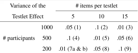
simulation design had 9 distinct conditions. In table 1, the whole design is shown. The numbers 1 to 9 in parenthesis refer to the numbering of the nine conditions.

Table 1

Table of Simulation Design

Variance of the Testlet Effect

# items per testlet

5 10 15

1000 .05 (1) .1 (2) .01 (3) # participants 500 .1 (4) .01 (5) .05 (6) 200 .01 (7a & b) .05 (8) .1 (9) Note. The latin square design limits the number of conditions needed, but still maximize the number of combination of conditions observed. The numbers in brackets () indicate the number of the condition.

Condition 7 was run two times, with different prior specifications for the testlet parameter under the conditional testlet model. They are indicated by 7a and 7b.

In order to investigate the effect of different priors on the parameter estimation under the conditional testlet model for conditions with little information, condition 7 was ran a second time, with different prior specifications. Condition 7a was run with the noninformative prior for the testlet parameter variance set to 0.01. Condition 7b, on the other hand, was run with an

Criteria

Through sampling from the posterior distributions of model parameters, parameter estimates were obtained. Calculating bias and mean squared error (MSE) of these parameters shows the accuracy of these parameter estimates. It is an indication of how well the two models each describe the data. The bias and mean squared error (MSE) were calculated for different model parameters obtained under the two models. Where applicable, the results were averaged across the test items and participants, to make the comparison more straightforward. Bias was calculated as the average difference between the true and estimated value;

Bias(bˆ_j) = 1 50

50

∑

(bˆ_jr−b_jr), (2)

where ˆb_jr is the estimated difficulty parameter for item j in replication r. b_jrepresents the true value of the difficulty parameter for item j in replication r. MSE was calculated similarly, with:

MSE(bˆ_j) = 1 50

50

∑

(bˆ_jr−b_jr)2. (3)

Bias and MSE were calculated for the discrimination parameter (a), the difficulty parameter (b), the ability parameter (θ). Furthermore, bias and MSE was calculated both for the variance of the testlet effect and the estimated individual testlet effects. Additionally, the mean absolute deviation of the individual testlet effects was calculated. This was done by:

mean absolute deviation(γˆ) = 1 50

50

∑

(|γˆr−γr|). (4)

MSE and bias of the two models are not on the same scale, artificially lowering the MSE and bias under the conditional testlet model by comparison. In order to make a fair comparison possible, the estimated testlet effects under both models were rescaled to be on the same scale. Outcomes on the testlet estimates given below are based on the rescaled values.

Another indicator of how well the models describe the data is the coverage rate. A Highest Postrior Density (HPD) interval was used. The interval gives an indication of the amount of times that the true value lies within the predicted interval. Both models are designed to have a 95% coverage rate. If this is lower, the true values do not lie within the predicted interval enough times. The lower the coverage rate, the less often we would find the true value to lie within the 95% HPD, given many replications. If the coverage is low, the model would claim to find the underlying true value more frequently than is actually warranted. A low coverage rate indicates a problem with the models functioning. It is predicted that the coverage rate under the marginal testlet model will be higher than the true 95%. This is not indicative of bad model functioning, since under the marginal testlet model observations are not restricted to be positively correlated within a testlet. This leads to a wider confidence interval. As the data is generated under the conditional testlet model, the coverage does not match up exactly.

The estimation of the MSE and bias was based on mean estimation. It was expected that the conditional testlet model would have a skewed posterior distribution of the variance parameter. If this is the case, mean estimation could lead to inaccurate estimations, as the mean would not represent the center of the distribution. Therefore, results were also obtained when using a mode estimation method. If the differences between the two estimations are large, this would indicate that the posterior distributions are skewed and the results may be imprecise. This was predicted for the conditional testlet model under small testlet variances. The Asselin de Beauville mode estimator (Poncet, 2012) was used to estimate the mode, and results obtained using both methods were compared.

Results

Table 2

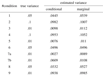
Estimated Testlet Variance for the Conditional and Marginal Model

#condition true variance

estimated variance conditional marginal

1 .05 .0445 .0539

2 .1 .0982 .1007

3 .01 .0098 .0112

4 .1 .0953 .1052

5 .01 .0076 .011

6 .05 .0496 .0496

7a .01 .0027 .0089

7b .01 .0609 .0108

8 .05 .0332 .0527

9 .01 .0938 .0985

Note. The average estimated testlet variances were recovered from the conditional and marginal testlet model. A value closer to the

true variance indicates better model performance

conditions were run again with the discrimination parameter fixed to 1. We think that this does not influence the outcomes in any meaningful way, though.

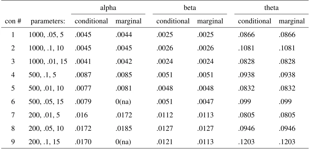
In all ten conditions parameter estimates were obtained. For the estimation of the model parametersa,b, andθ, very little to no differences were found between the estimation methods under the two models. Estimates for bias and MSE of these parameters are displayed in the Appendix, Table 8 and Table 7 respectively. Small differences were observed between the bias of a, but we think they are not big enough to be relevant.

Table 3

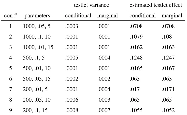
MSE of True Parameters and Estimated Posterior Mean for the testlet variance and Testlet Effects

testlet variance estimated testlet effect con # parameters: conditional marginal conditional marginal

1 1000, .05, 5 .0003 .0001 .0708 .0708

2 1000, .1, 10 .0001 .0001 .1079 .108

3 1000, .01, 15 .0001 .0001 .0162 .0163

4 500, .1, 5 .0005 .0004 .1248 .1247

5 500, .01, 10 .0001 .0001 .0165 .0167

6 500, .05, 15 .0002 .0002 .063 .063

7 200, .01, 5 .0001 .0004 .017 .0171

8 200, .05, 10 .0006 .0003 .065 .065

9 200, .1, 15 .0008 .0007 .1055 .1052

Note. The MSE for the testlet variance and the estimated testlet effect, estimated under the conditional and the marginal testlet model.

marginal testlet model, on the other hand, the testlet variance tended to be slightly overestimated. Only in conditions 6, 7a, and 9, the testlet variance was underestimated. In general, the estimates were very precise under the marginal testlet model.

We see that the parameter estimates, under the marginal testlet model, are slightly different for the conditions 7a and 7b (Table 2, Table 5). As the estimates were obtained while using a constant seed, we would expect the exact same data for both conditions under the marginal testlet model, as the only difference between the two conditions (informative vs. uninformative prior for the testlet effect) does not apply to the marginal testlet model. But because the generated datasets were analysed under both testlet models within the same run of the program, the changes in estimation under the conditional testlet model have an impact on the results of estimation under the marginal testlet model. Because the estimations rely on random draws, these slight variations in results are expected.

Table 4

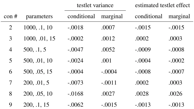
Bias of True Parameters and Estimated Posterior Mean for the Testlet Variance and Testlet Effects

testlet variance estimated testlet effect con # parameters conditional marginal conditional marginal

2 1000, .1, 10 -.0018 .0007 -.0015 -.0015

3 1000, .01, 15 -.0002 .0012 .0002 .0003

4 500, .1, 5 -.0047 .0052 -.0009 -.0008

5 500, .01, 10 -.0024 .001 -.0004 -.0002

6 500, .05, 15 -.0004 -.0004 -.0008 -.0007

7 200, .01, 5 -.0073 -.0011 .0002 .0003

8 200, .05, 10 -.0168 .0027 .0028 .0026

9 200, .1, 15 -.0062 -.0015 -.0013 -.0013

Note. The bias for the testlet variance and the estimated testlet effect, estimated under the conditional and the marginal testlet model.

conditional testlet model, bias was smaller than under the marginal testlet model for all conditions. In fact, the bias was negative, ranging from−.0168 in condition 8 to−.0002 in condition 3. For the testlet effects themselves, we see lower values of bias under the conditional testlet model in conditions 4, 5, 6, and 7. This means that under the conditional testlet model, the estimates of the testlet effects and the testlet variance were slightly closer to the true values. For the testlet effects, the mean absolute deviation is shown in Table 5. There are very little

differences. The estimates obtained under the marginal testlet model have nearly the same testlet estimates.

The coverage rate under the conditional testlet model was not satisfactory for most

conditions. As can be seen in Table 6, under the conditional testlet model, a lower coverage rate for most conditions was found. Only in condition 2 was the coverage rate higher than the target 95%, with a coverage of 100%. The next highest is in condition 3, with a coverage of 90%. In the other conditions, low coverage rates were found. This indicates that the true value did not fall within the estimated confidence interval.

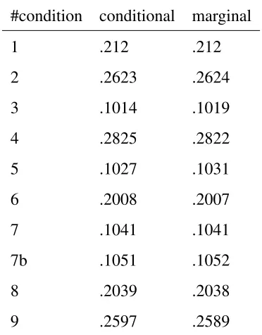
Table 5

Mean Absolute Deviation of the Estimated Testlet Effects

#condition conditional marginal

1 .212 .212

2 .2623 .2624

3 .1014 .1019

4 .2825 .2822

5 .1027 .1031

6 .2008 .2007

7 .1041 .1041

7b .1051 .1052

8 .2039 .2038

9 .2597 .2589

Note.The mean absolute deviation. The rescaled effects showed nearly no difference between estimates under the two models.

conditions but 6 and 9, the coverage rate was 100%. In condition 6 and 9, the coverage rate is 94% and 96% respectively. These were the conditions where the discrimination parameter was adjusted, which could explain the difference to coverage rates in the other conditions, under the marginal testlet model.

Table 6

Coverage of the 95% Confidence Interval

#condition conditional marginal

1 .78 1.00

2 1.00 1.00

3 .90 1.00

4 .86 1.00

5 .76 1.00

6 .88 .94

7a .10 1.00

7b 0 1.00

8 .76 1.00

9 .86 .96

Note.Convergence was calculated using a HPD function. The coverage under the conditional testlet model is too low. Especially condition 7a and 7b. Under the marginal model, coverage is higher than the

target coverage.

.

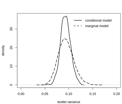
0.00 0.05 0.10 0.15 0.20

0

10

20

30

testlet variance

density

conditional model

marginal model

Figure 1. Density of the sampled testlet variance estimates from the posterior distribution under the conditional and marginal testlet model. Under the conditional testlet model, estimates show a higher density and a narrower variance than under the marginal testlet model. The 14th

2000 4000 6000 8000 10000

−0.05

0.10

0.20

0.30

testlet v

ar

iance

conditional testlet algorithm

2000 4000 6000 8000 10000

−0.05

0.10

0.20

0.30

iterations

testlet v

ar

iance

marginal testlet algorithm

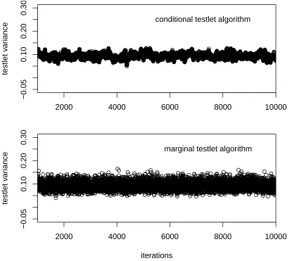
Figure 2. The Figure shows the samples from the posterior distribution of the testlet variance. The MCMC chain goes from left to right. The x-axis goes from 1000-10,000, as the first 1000

iterations are used to reach the posterior distribution. The 14th replication of condition 2 was used.

For some conditions, we could not obtain reliable estimates for the conditional testlet model. This varies per condition, with some more affected than others.

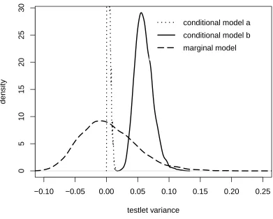
−0.10 −0.05 0.00 0.05 0.10 0.15 0.20 0.25

0

5

10

15

20

25

30

testlet variance

density

conditional model a

conditional model b

marginal model conditional model a

conditional model b

marginal model

2000 4000 6000 8000 10000

−0.05

0.05

0.15

0.25

testlet v

ar

iance

conditional testlet algorithm − uninformative prior

2000 4000 6000 8000 10000

−0.05

0.05

0.15

0.25

testlet v

ar

iance

conditional testlet algorithm − informative prior

2000 4000 6000 8000 10000

−0.05

0.05

0.15

0.25

iterations

testlet v

ar

iance

marginal testlet algorithm

Figure 4. The Figure shows the samples from the posterior distribution of the testlet variance. It is shown at the top how, with the specification of a non-informative prior, the algorithm cannot sample from the posterior distribution. The 14th replication of condition 7 was used.

Under the marginal testlet model, on the other hand, reliable estimates of the testlet

is symmetrical, with its mean around zero. The highest density is only just below 10 and the distribution is larger. Compared to the distribution of values in Figure 1, under the marginal testlet model, the distribution is much wider. This is not surprising, as there is much less information available, which introduces more uncertainty into the estimation. Again, the same can be seen in the density plot in Figure 4 in the bottom figure. The algorithm draws estimates from the posterior distribution of the testlet variance with a wider distribution. We can see how under the marginal testlet model, estimates can be sampled lower than zero.

In all of the replications of condition 7a, the algorithm failed to obtain good parameter estimates for the testlet variance. In other conditions, like condition 8, only in some of the

replications similar difficulties were observed. Some of the replications performed well, similar to the distributions shown in Figure 1, and in others the distribution failed to show good variance.

The mean and mode estimations for the MSE and biases showed very small differences. This means that the mean and the mode did not vary from each other strongly. This did not support the hypothesis that the conditional testlet model would show strongly skewed posterior distributions. Therefore, it was viable to use mean estimation for the bias and mean squared error.

Discussion

This article presents evidence that, first, under the marginal testlet model, accurate

parameters for data generated under the conditional testlet model can be estimated, and, second, that the marginal testlet model functions better than the conditional testlet model under conditions with little information and small testlet variances.

The second main point of this paper was to show the marginal testlet models applicability for datasets with less available information. It was shown that under the conditional testlet model, a point is reached at which its outcomes are highly reliant on the testlet effect prior specification. Condition 7a and 7b showed how we are not able to obtain reliable parameter estimates if the information in the dataset is too little. It was shown that under the marginal testlet model, reliable estimates are delivered in conditions with few participants, small testlet variance, and few items per testlet. The conditional testlet model did function better in some regards than was expected beforehand. The issues in obtaining reliable posterior estimates under the conditional testlet model did not have a clearly visible effect on the bias and MSE of model parameters.

Nevertheless, the coverage rate and the estimated testlet variances, as well as the density plots, are evidence of the limited usefulness of the conditional testlet model.

An issue with the current research was the fact that the marginal testlet model had problems functioning under rare conditions. It is our belief, though, that this issue is not indicative of an underlying problem with the marginal testlet model, but merely an issue with the current estimation program used. This issue should be resolved in further iterations of the program. Furthermore, the temporary fix of settinga_j to 1 did not influence the current results in a meaningful way.

References

Wainer, H., & Kiely, G. L. (1987). Item clusters and computerized adaptive testing: A case for testlets.Journal of Educational measurement, 24(3), 185-201.

Wainer, H., Bradlow, E. T., & Wang, X. (2007). Testlet response theory and its applications. Cambridge University Press.

Bradlow, E. T., Wainer, H., & Wang, X. (1999). A Bayesian random effects model for testlets. Psychometrika, 64(2),153-168.

Wang, X., Bradlow, E. T., & Wainer, H. (2002). A general Bayesian model for testlets: Theory and applications.ETS Research Report Series,2002(1).

Plummer, M., Best, N., Cowles, K. & Vines, K. (2006). CODA: Convergence Diagnosis and Output, Analysis for MCMC, R News, vol 6, 7-11

Appendix

Table 7

Mean Squared Error Between True Parameters and Estimated Posterior Means

alpha beta theta

con # parameters: conditional marginal conditional marginal conditional marginal

1 1000, .05, 5 .0045 .0044 .0025 .0025 .0866 .0866

2 1000, .1, 10 .0045 .0045 .0026 .0026 .1081 .1081

3 1000, .01, 15 .0041 .0042 .0024 .0024 .0828 .0828

4 500, .1, 5 .0087 .0085 .0051 .0051 .0938 .0938

5 500, .01, 10 .0077 .0081 .0048 .0048 .0832 .0832

6 500, .05, 15 .0079 0(na) .0051 .0047 .099 .099

7 200, .01, 5 .016 .0172 .0112 .0113 .0805 .0805

8 200, .05, 10 .0172 .0185 .0127 .0127 .0946 .0946

9 200, .1, 15 .0170 0(na) .0121 .0113 .1203 .1203

Table 8

Bias Between True Parameters and Posterior Estimate for the Model Parameters for the

Conditional and Marginal Testlet Model

alpha beta theta

con # parameters conditional marginal conditional marginal conditional marginal

2 1000, .1, 10 .0043 .0044 -.0026 -.0026 .0001 .0001

3 1000, .01, 15 .0039 .0041 .002 .002 .0001 .0001

4 500, .1, 5 .0084 .0082 .0001 .0001 .0001 .0001

5 500, .01, 10 .0075 .0079 .0029 .003 -.0001 -.0001

6 500, .05, 15 .0077 0(na) .0033 .0029 -.0001 -.0001

7 200, .01, 5 .0158 .0169 .0008 .0005 .0001 .0001

8 200, .05, 10 .0168 .018 -.0013 -.0012 .0001 .0001

9 200, .1, 15 .0166 0(na) .0028 .0018 .0001 .0001