University of Warwick institutional repository:
http://go.warwick.ac.uk/wrap
A Thesis Submitted for the Degree of PhD at the University of Warwick
http://go.warwick.ac.uk/wrap/55659
This thesis is made available online and is protected by original copyright.
Please scroll down to view the document itself.
by
Lieke van Spaandonk, MSc
Thesis
Submitted to the University of Warwick
for the degree of
Doctor of Philosophy
Department of Physics
List of Tables vii
List of Figures viii
Acknowledgments xi
Declaration and published work xii
Abstract xiii
Glossary and abbreviations xiv
Chapter 1 Cataclysmic Variables 1
1.1 Binaries . . . 1
1.1.1 Nomenclature . . . 1
1.1.2 Binary geometry . . . 2
1.1.3 Roche lobe geometry . . . 3
1.2 Binary evolution . . . 3
1.2.1 Accretion and disc formation . . . 5
1.2.2 CV evolution . . . 5
1.2.3 Angular momentum loss . . . 8
1.2.4 Mass transfer . . . 10
1.2.5 Period distribution . . . 11
1.3 Dwarf Novae . . . 14
1.3.1 Disc outburst . . . 15
1.3.2 Superhumps . . . 17
1.4 Setting the scene . . . 21
Chapter 2 Methods 23 2.1 Spectral features in CVs . . . 23
2.2 Time-resolved spectroscopy . . . 26
2.2.1 Spectroscopy . . . 26
2.3.3 Doppler tomography . . . 36
2.3.4 Gravitational redshift . . . 42
2.4 Irradiation modelling . . . 44
2.4.1 K-correction . . . 44
2.4.2 Radial velocity of the emission component . . . 45
2.4.3 Line strength variation . . . 48
2.5 New diagnostics . . . 48
2.5.1 Motivation . . . 48
2.5.2 Emission line broadening . . . 50
2.5.3 Emission line broadening as function of the inclination . . . 51
2.5.4 Emission line models . . . 51
2.5.5 Diagnostic power of Ca II . . . 53
2.6 The plan for constraining q . . . 54
2.6.1 MeasuringK2 . . . 54
2.6.2 MeasuringK1 . . . 54
2.6.3 New lines . . . 55
Chapter 3 GW Lib I 56 3.1 Introduction . . . 56
3.2 Observations and reduction . . . 57
3.2.1 Telescopes and instruments . . . 57
3.2.2 Reduction . . . 58
3.3 GW Lib in outburst . . . 60
3.3.1 Spectral evolution . . . 60
3.3.2 Time-resolved spectra . . . 65
3.4 GW Lib post outburst . . . 70
3.4.1 Emission from the secondary . . . 71
3.4.2 Emission from the accretion disc . . . 73
3.4.3 Systemic velocity . . . 75
3.4.4 System parameters . . . 76
4.1 Introduction . . . 82
4.2 Observations and reduction . . . 82
4.3 Gravitational redshift for Mg II . . . 83
4.3.1 vMgII . . . 85
4.3.2 vgrav(donor) . . . 86
4.3.3 The systemic velocityγ . . . 86
4.3.4 The implied WD mass . . . 87
4.3.5 System parameters and WD spin . . . 87
4.4 Discussion . . . 89
Chapter 5 Ca II survey I 92 5.1 Observations and reduction . . . 92
5.1.1 Target Selection . . . 92
5.1.2 WHT/ISIS . . . 93
5.1.3 VLT/UVES . . . 96
5.2 EW measures . . . 97
5.3 The survey . . . 97
5.3.1 Time-resolved data analysis . . . 98
5.3.2 GW Lib . . . 102
5.3.3 V844 Her . . . 104
5.3.4 V455 And . . . 105
5.3.5 ASAS 0025+1217 . . . 107
5.3.6 WZ Sge . . . 109
5.3.7 V1108 Her . . . 114
5.3.8 HS 2219+1824 . . . 115
5.3.9 OY Car . . . 116
5.3.10 V632 Cyg . . . 119
5.3.11 UV Per . . . 121
5.3.12 IX Dra . . . 123
5.3.13 TY Psc . . . 123
5.3.14 GD 552 . . . 126
5.3.15 IY UMa . . . 127
5.3.16 HT Cas . . . 128
5.4 Summary . . . 137
Chapter 6 Ca II survey II 145 6.1 EW measures . . . 145
6.2 Disc features in CVs . . . 148
6.3 Donor features in CVs . . . 150
6.4 Correlations and trends . . . 153
6.5 Evolution of Ca II . . . 159
6.5.1 GW Lib . . . 161
6.5.2 V455 And . . . 165
6.6 Summary . . . 170
Chapter 7 Ca II survey III 172 7.1 Measuring K1 . . . 172
7.1.1 Methods . . . 173
7.1.2 Balmer versus Ca II . . . 174
7.2 Measuring K2 . . . 175
7.2.1 Methods for measuringKem orKabs . . . 175
7.2.2 Balmer versus Ca II . . . 178
7.2.3 K-correction . . . 179
7.3 Constraining q . . . 180
7.3.1 ConstrainingK2 . . . 181
7.3.2 Constrainingq . . . 182
7.3.3 Notes on specific systems . . . 190
7.4 Ca II as tracer ofq in DNe? . . . 196
Chapter 8 Discussion and Conclusion 198 8.1 Motivation . . . 198
8.2 GW Lib . . . 199
8.3 The survey . . . 202
8.3.1 Ca II emission . . . 202
8.3.2 MeasuringK1 . . . 203
8.3.5 Period evolution combined withq. . . 205
8.4 Epsilon(q) relation . . . 206
8.5 Conclusion . . . 209
8.6 Future projects . . . 209
3-1 Observations of GW Lib . . . 59
3-2 ew of various emission lines as function of the outburst . . . 66
3-3 Radial velocity curve parameters on 2007 April 15. Note,φ0 is anchored to the ephemeris, but due to lack of precision, arbitrary at this point. . 68
3-4 Radial velocity curve parameters on 2007 June 25. . . 72
3-5 Derived system parameters for GW Lib . . . 78
4-1 Details of observations. . . 83
4-2 System parameters for GW Lib. . . 89
5-1 Period information of the observed systems . . . 94
5-2 WHT - ISIS 2000 observations - P33 . . . 94
5-3 VLT - UVES 2001 observations - 66.D-0505(A) . . . 94
5-4 WHT - ISIS 2007 observations - P19 . . . 95
5-5 WHT - ISIS 2008 observations - P35 . . . 95
5-6 WHT - ISIS 2009 observations - P26 . . . 96
5-7 EW measurements for Balmer . . . 98
5-8 EW measurements for Calcium . . . 99
5-9 Where can I find: section, details of observations, spectra and Doppler maps of the systems. . . 99
5-10 Radial velocity measurements I . . . 142
5-11 Radial velocity measurements II . . . 143
5-12 Radial velocity measurements III . . . 144
6-1 System parameters and emission line features for the surveyed CVs . . . 149
6-2 WHT - ISIS GW Lib and V455 And observations. . . 161
6-3 EW measurements for GW Lib and V455 And as a function of time . . 163
7-1 Radial velocity measurements and K-correction . . . 176
1-1 Left: Artist’s impression of a CV.Right: Roche Geometry . . . 4
1-2 Schematic illustration of the formation of an accretion disc. . . 6
1-3 CV evolution channel . . . 7
1-4 Period evolution versus accretion rate for a CV . . . 9
1-5 Period distribution of CVs . . . 12
1-6 Lightcurves of Z Cam, VW Hyi and GW Lib . . . 15
1-7 Disc instability as a function of surface density and temperature. . . 17
1-8 Lichtcurve of V455 And . . . 18
1-9 Example of sphsimulations . . . 19
1-10 Left: Porb versus the superhump period excess . Right: Mass ratio q versus the superhump period excess . . . 20
1-11 , q calibrators with theoretical prediction . . . 21
2-1 Spectrum displaying the principal components of a cataclysmic variable: WD, donor and accretion disc . . . 24
2-2 Formation of the double peaked profile from the accretion disc . . . 25
2-3 Data reduction example displaying the raw frame, extracted spectrum and wavelength calibrated spectrum of UV Per . . . 27
2-4 fwhm,ew,fwziand 2-Gaussian fit to spectral profiles . . . 32
2-5 Diagnostic diagram for OY Car . . . 35
2-6 Conversion from space coordinates to velocity coordinates . . . 37
2-7 Example of the Doppler map for UV Per . . . 39
2-8 Centre of symmetry method for UV Per . . . 41
2-9 Influence ofγ on the Centre of Symmetry method for UV Per . . . 42
2-10 Dependence of the measured radial velocity amplitude of the emission/absorption components on the location on the donor surface . . . 45
2-11 Kem as a function of various model parameters . . . 47
2-12 Synthetic light curve example . . . 49
2-13 Example line profiles from the disc for hydrogen and calcium . . . 52
3-4 Radial velocity curves for He ii and Hβ . . . 69
3-5 The average normalisedI-band spectrum of GW Lib on July 24, 2007 . 73 3-6 Trails and Doppler maps for Balmer and CaII . . . 74
3-7 Radial velocity curves of Hβ and Ca ii . . . 75
4-1 Average spectrum of GW Lib on the 16th of May 2002 . . . 84
4-2 Radial velocity curve of the Mg ii absorption line (the orbital coverage is plotted twice) with the best fit derived from Monte-Carlo simulations (K= 13±2 km s−1). . . 86
4-3 Mass-radius relationship for the measuredvgrav . . . 88
5-1 Average spectra of GW Lib, WZ Sge and HS 2219 . . . 103
5-2 The average spectra of V1108 Her, V844 Her, GD 552 and IX Dra . . . 104
5-3 The average spectra of V455 And and SU UMa . . . 106
5-4 The average spectra of YZ Cnc, ASAS 0025 and IY UMa . . . 107
5-5 Residual Balmer and Caii Doppler maps for ASAS 0025 . . . 108
5-6 Balmer and Ca ii trails and Doppler maps of GW Lib, V844 Her, V455 And and ASAS 0025 . . . 110
5-7 Trails and Doppler maps for WZ Sge . . . 113
5-8 Hβ Doppler maps of HS 2219 . . . 116
5-9 Average spectrum of OY Car . . . 117
5-10 Balmer, Caii and Potassium trails and Doppler maps for OY Car . . . 120
5-11 Zoom of the Hα, Caii and K Doppler maps for OY Car . . . 121
5-12 Average spectrum of UV Per showing the Mgiiabsorption . . . 122
5-13 The average spectra of V632 Cyg, UV Per, TY Psc and HT Cas . . . . 124
5-14 Balmer and Caiitrailed spectra and Doppler maps of WZ Sge, HS 2219, UV Per and TY Psc . . . 125
5-15 Balmer and Caiitrails and Doppler maps of GD 552, IY UMa, HT Cas and SU UMa . . . 131
5-16 The average spectra of SS Cyg and IP Peg . . . 133
6-2 Light curve variations for GW Lib and SS Cyg . . . 152
6-3 EW ratios as a function of Porb . . . 155
6-4 EW ratios as a function of i,MWD and TWD . . . 156
6-5 Relations between MWD,TWD and Porb . . . 158
6-6 ew as a function ofi . . . 160
6-7 Average spectra of GW Lib as a function of time . . . 162
6-8 The Doppler maps of GW Lib at 4 different epochs . . . 164
6-9 Periodogram for GW Lib . . . 166
6-10 Average spectra of V455 And as a function of time . . . 167
6-11 The average red spectrum of V455: Caii or Paschen? . . . 168
6-12 ew ratio as a function of time since last outburst . . . 170
7-1 Calculated K-correction as a function ofq for OY Car . . . 180
7-2 The K1, qplane for OY Car, with dynamical constraints . . . 183
7-3 The K1, qplane for GW Lib . . . 184
7-4 The K1, qplane for ASAS 0025 . . . 184
7-5 The K1, qplane for for WZ Sge . . . 185
7-6 The K1, qplane for HS 2219 . . . 185
7-7 The K1, qplane for OY Car . . . 186
7-8 The K1, qplane for UV Per . . . 186
7-9 The K1, qplane for TY Psc . . . 187
7-10 TheK1, qplane for IY UMa . . . 187
7-11 TheK1, qplane for HT Cas . . . 188
7-12 TheK1, qplane for SU UMa . . . 188
7-13 TheK1, qplane for YZ Cnc . . . 189
7-14 TheK1, qplane for IP Peg . . . 189
7-15 TheK1, qplane for SS Cyg . . . 190
7-16 The Caii and Ca K Doppler maps for SS Cyg . . . 193
8-1 Orbital Period versus q, comparing our solutions with binary evolution models . . . 206
8-2 Mass ratio versus superhump excess, comparing our solutions with previ-ous studies . . . 207
How I wonder what you are!
I would like to take this opportunity to wholeheartedly thank Danny Steeghs for his supervision, guidance and scientific support during the past three and a half years. The Astronomy and Astrophysics group at the University of Warwick provided a comfortable and stimulating environment for me to do my work and for that, I want to thank all academic staff, post-docs and PhD students. Extra gratitude goes to Tom Marsh, for the additional supervision. I would like to thank Joao, Jon and Simon for the endless provision of chocolate, coffee, programming support, inappropriate conversation and general distraction throughout the years, and Sandra for the, sometimes, much needed girly talk about dresses and shoes.
A great thanks to my social ‘support’ group, for providing me with friendship through-out the years, independent of distance. In no particular order1: Dean, Ulrika, Solveig, Jos´e, Lisa, Stephanie and Ruth.
Als laatste, maar zeker niet als minste, wil ik graag mijn familie bedanken. Vaders en moeders, ik kan jullie niet dankbaar genoeg zijn voor de onophoudelijke steun en toeverlaat tijdens mijn ontdekkingsreis naar de wonderen van de natuur. Thijs, Koen en Guus, ik zal jullie gezichten tijdens mijn Masters uitreiking nooit vergeten en het zet me regelmatig weer met beide beentjes stevig terug op aarde. Oma, dank je wel voor alle koffie, kapsels en planten, maar vooral voor de Brabantse gezelligheid. Ik kom snel weer ‘blieken en gebruiken’ op de boulevard. En Andrew, ook al heb je me laten zien dat wonderen heel dicht bij huis gevonden kunnen worden en hou ik heel veel van je, ik ben je niet dankbaar voor het onophoudelijk neuri¨en van ‘Twinkle, twinkle, little star’, hoe toepasselijk ook het ook mag zijn.
I declare that the work presented in this thesis is my own except where stated otherwise, and was carried out entirely at the University of Warwick, during the period October 2007 to March 2011, under the supervision of Dr. D.T.H. Steeghs. The research reported here has not been submitted, either wholly or in part, in this or any other academic institution for admission to a higher degree.
The following Chapters of this thesis are based on refereed publications:
• Chapter3is based on van Spaandonk, L., Steeghs, D., Marsh, T. R., Torres, M. A. P.Time-resolved spectroscopy of the pulsating CV GW Lib, 2010, Monthly Notices of the Royal Astronomical Society,401, 1857
• Chapter4is based on van Spaandonk, L., Steeghs, D., Marsh, T. R., Parsons, S.G.
The mass of the white dwarf in GW Libra, 2010, Astrophysical Journal Letters, 715, L109
Conference contributions based on this thesis are:
• NAM, Belfast, 2008. Poster: Time-resolved spectroscopy of the pulsating CV GW
Lib.
• Wild Stars in the Old West II, Tucson Arizona, USA 2009. Oral Presentation: Ca II Spectroscopy of Short Orbital Period CVs.
• IAC Winterschool, Tenerife 2009. Poster: Mapping Emission Line Features in
CVs.
• NAM, Glasgow, 2010. Poster: Binary populations in sdss: A new diagnostic for system parameters of evolved white dwarf binaries.
I acknowledge with thanks the variable star observations from theaavsoInternational
Theory predicts that a large fraction of CVs should have passed through the min-imum period. The Sloan Digital Sky Survey (sdss) sample is finally unearthing these
systems in large numbers. But due to their faint donor stars, the orbital period is often the only measurable system parameter for most CVs. The indirect measurable of the superhump period, and hence superhump excess, could potentially provide an indication of the mass ratio of the systems via the empirical relation between the two observables. While this relation is potentially very useful for the determination of mass ratios, the large scatter in the calibrators, especially at the low mass ratio end, prohibits a direct conversion between easy to measure light curve variability and the much sought after mass ratio. To place a short period CV firmly on the evolutionary track (e.g pre- or post bounce systems), more direct methods to determine the mass ratio are required, as well as a better calibration and validation of the relation between the superhump excess and mass ratio.
We can achieve this, by constraining the mass ratios of short period CVs using dynamical constraints on the radial velocities of the binary components. The radial velocity of the WD (K1) is only occasionally directly measurable as the WD features are typically swamped by the strong disc features. As the disc is centred on the WD, measuring the disc radial velocity can give an indication of the WD radial velocity, but these measures tend to be biased by hotspots and other asymmetries in the disc.
Measuring the radial velocity of the donor star (K2) is less straightforward and nor-mally performed by either measuring the radial velocity of the donor absorption lines for earlier type donor stars, or via emission lines associated with the donor star, if irradiated by the disc and WD. The first method fails in short period CVs as the faint features from the late type donors in these systems are concealed in the accretion and WD dominated optical spectrum, even at very low mass loss rates. The second method comes with tight timing constraints as the irradiated donor is generally only visible on top of the double peaked disc emission shortly after outburst and data needs to be obtained via target of opportunity programs.
In this thesis, we present a spectroscopic survey of short periods CVs and explore new techniques in addition to the traditional methods for the determination of the radial velocity components. We combine these new methods with the exploitation of the more ‘exotic’ Caiitriplet lines in the I-band in addition to the commonly used Balmer lines.
We will show that, while it suffers from some of the same systematics as the Balmer lines, we can measure K1 better in Ca ii than in Balmer, especially when exploiting Doppler maps for these measures. More importantly for many systems, donor emission is visible in the Ca ii lines, which provides us with measures for the radial velocity
WD white dwarf
CV cataclysmic variable
DN dwarf nova
FWHM full width at half maximum
EW equivalent width
FWZI full width at zero intensity
RLOF Roche lobe over flow
MB magnetic braking
GWR gravitational wave radiation
LMXB low mass X-ray binary
CCD charge coupled device
RMS root mean square
RV radial velocity
MEM maximum entropy map
COS centre of symmetry
DD diagnostic diagram
S/N signal to noise
RON read out noise
VLT Very Large telescope
WHT William Herschel telescope
Cataclysmic Variables
1.1
Binaries
Roughly half of the stars visible at night are multiple systems containing two or more stars orbiting around a common centre of mass due to their mutual gravitational attrac-tion. The diversity of binary systems is explained by a broad range of initial parameters: e.g. initial masses of the individual components, age and hence evolution, the separa-tion, the influence of the individual evolution on the system etcetera. Understanding these parameters provides crucial information about binary and stellar evolution since all stellar population models are affected by binary interactions.
1.1.1 Nomenclature
Out of the many different binary configurations, this thesis only concerns the eclipsing and the spectroscopic binaries at short orbital periods containing an evolved compact object.
• Eclipsing binaries are those binaries that have their orbital plane orientated
along our line of sight, showing periodic dips in brightness as one of the components passes in front of the other, hence blocking its light. These eclipses in the light curves do not only reveal the presence of the secondary star but also contain information on the relative effective temperatures and radii of both stars, as they are a function the eclipse width and depth (e.g. Parsons et al. 2010, Littlefair et al. 2008).
• Spectroscopic binaries show periodic Doppler shifts in their emission and/or
– Single line binariesonly display the spectral features of one binary compo-nent. Single lined binaries also include planetary systems, as the presence of the (undetectable) planet is revealed by the periodical wobble of the central star.
– Double line binariesshow the spectral features of both components, with their respective Doppler shifts out of phase by ∆φ = 0.5. The ratio of the radial velocities is a measure of the mass ratio of the components, see next section (1.1.2).
1.1.2 Binary geometry
Kepler’s third law states that the orbital period squared (Porb2 ) of a body around its centre of mass, is directly proportional to the semi-major axis of the orbit cubed (a3;
Kepler et al. 1619). In this scenario, gravity provides the centripetal force required to keep the system im circular motion. The relation for two bodies around a common centre of mass, is given by:
Porb2 = 4π 2
G(M1+M2)
a3 (1-1)
with M1 the primary mass, M2 the secondary mass and M2 < M1 for the systems concerned in this thesis. We can draw up the next set of equations for the components as they rotate around their common centre of mass:
a = a1+a2, (1-2)
M1a1 = M2a2, (1-3)
(1-4)
witha1 and a2 the distance from the primary and secondary to the centre of mass. The true circular velocities for the components are given by
v1 = 2πa1
Porb
, (1-5)
v2 = 2πa2
Porb
. (1-6)
Solving the latter two for a1 and a2 and substituting into the mass ratio q ≡M2/M1, gives the relation between the mass ratio and the velocities: q = v1/v2. The velocity is projected along the line of sight, with the measured radial velocity K1,2 =v1,2sini, with ithe inclination angle of the system. Thus, we can express the mass ratio as the ratio of the observed velocities:
q = M2
M1 = K1
K2
velocity of one component is measurable, the mass function is defined as:
f(M) = M1sin 3i (1 +q)2 =
PorbK23
2πG (1-8)
which, as sin3i 6 1 and (1 +q)2 > 1, sets a lower limit for the mass of the primary component.
1.1.3 Roche lobe geometry
The geometry of close binaries is generally talked about in terms of the Roche geometry. For a Cartesian coordinate frame co-rotating with the binary, the origin at the primary and thex-axis aligned with the centres of the components, they-axis in the direction of the orbital motion and thez-axis perpendicular to the orbital plane, the total potential can be expressed as the sum of the gravitational potential of the individual stars and the effective potential of the centrifugal force. This is known as the Roche potential (Frank et al.,1992):
ΦR=−
GM1
(x2+y2+z2)1/2 −
GM2
((x−a)2+y2+z2)1/2 − 1 2Ω
2 orb
(x−µa)2+y2
. (1-9)
This equation is solely determined by the binary separation and the component masses, with µ = M2/(M1 +M2) and the orbital period via Ωorb = 2π/Porb. The Roche equipotentials (ΦR= const), are set by the mass ratio, relative to the binary separation
(Figure 1-1). Close to the components, these potentials are nearly circular as they are mostly governed by the component’s mass, but further outwards the gravitational potential of the second mass distorts this shape. The inner most equipotential, where the surfaces of the two individual stars just touch as the forces cancel in the inner Lagrangian point (L1), is known as the Roche Lobe and only within this equipotential material is gravitationally bound to the parent star.
If the surface of a star expands beyond its Roche lobe, material is no longer gravita-tionally bound to that star and when entering the lobe of the companion star, material will be gravitationally bound to the latter instead. The net result is a flow of material from lobe to lobe, throughL1, called Roche lobe over flow (rlof).
1.2
Binary evolution
2.0 1.5 1.0 0.5 x/a0.0 0.5 1.0 1.5 2.0 2.0
1.5 1.0 0.5 0.0 0.5 1.0 1.5 2.0
y/a L3 WDCoM L1 MS L2
L4
L5
Figure 1-1: Left: Artist’s impression of the CV SDSS 1035+055 showing the donor star (in this case a brown dwarf), the mass transfer stream, the disc around the WD and the hotspot - where the stream impacts the disc (Courtesy Stuart Littlefair). Right: Roche Equipotentials for a system with mass ratio q = 0.2. Indicated are the positions of the primary and secondary star and the centre of mass. Also indicated are the 5 Lagrangian points. The Inner Lagrangian point L1 lies between the two masses. For the two outer Lagrangian points, L2 lies behind the smaller mass, on the line determined by the two masses, and L3 lies behind the larger mass. L4 and L5 are positioned at the vertical corners of the two equilateral triangles with as shared base the line between the centres of the two stars, with L4 leading the motion of the orbit andL5 laging behind.
• Detached binaryif both components have R∗ < RL.
• Contact binary if both components haveR∗=RL.
• Semi-detached binaryif one component has R∗ < RL and the otherR∗ > RL. In these casesrlof normally occurs.
Throughout its evolution, a binary can transform through these stages, depending on the initial masses and separation.
This thesis concerns the semi-detached binaries which contain accretion discs, a result of the mass transfer through L1. The Roche geometry is too difficult to solve analytically, hence approximations for numerous parameters have been derived which are generally accurate to ∼ 1%. Various approximations using the observables of the binary (K1,K2 and q=K1/K2) are given in chapter 2 inWarner(1995). For example, the distance from L1 to the centre of the primary, RL1, is given by:
RL1
which can be approximated for 0< q <∞(equation 2.5c):
R2
a =
0.49q2/3
0.6a2/3+ ln(1 +q1/3). (1-11)
1.2.1 Accretion and disc formation
The donor star loses gas from its Roche lobe, as it flows throughL1 into the Roche lobe of the primary at roughly the sound speed in the gas, which is set by the temperature of the donor’s atmosphere. The Coriolis force deflects the now free falling steam line and the material cannot fall straight onto the primary but sweeps past. As the particles in the stream do not have enough energy to escape the Roche lobe, they will be deflected close to the lobe surface and close in on themselves (top line, Figure 1-2). The material will settle into a Keplerian orbit around the primary, with the same angular momentum as the initial angular momentum of the material at the L1 point: at the circularisation radius. The Keplerian orbital velocity is given by:
Ωorb(r) =
GM
r3
1/2
, (1-12)
and, for mass ratios between 0.05 < q < 1, the circularisation radius can be approxi-mated by:
rcirc
a = 0.0488q
−0.464 (1-13)
(equation 2.14 from Warner 1995; second line, Figure 1-2). Different Keplerian radii have different Kepler velocities, hence the ring will experience friction between material at slightly different radii, which heats the gas. Radiation carries away the released potential energy, which causes the material to move to smaller radii. To conserve angular momentum, material also has to move towards larger radii, spreading the ring into a disc (third line, Figure 1-2). As angular momentum flows outwards through the disc, material can flow inwards and ultimately accrete onto the primary. The maximum disc radius is determined by tidal interactions with the secondary as it soaks up angular momentum. This radius is given by equation 2.61 from Warner(1995):
rtidal
a =
0.60
1 +q (1-14)
and is valid for 0.03< q <1. See bottom two lines in Figure 1-2.
1.2.2 CV evolution
Figure 1-2: Schematic illustration of the for-mation of an accretion disc (Figure 1 from
Verbunt 1982). From top to bottom: Top line: Initial stream trajectory due to Coriolis forces and the gravitational field. Second line: Formation of a ring at the circularisation radius.
Third line: Due to viscosity the disc spreads into a ring.
Fourth line: Disc forms with the outer ra-dius set by tidal interactions with the sec-ondary.
Bottom line: Side view.
Roche lobe overflow. The secondary star is typically a main sequence star.
CVs are formed through the evolutionary channel depicted in Figure 1-3, starting with a binary containing one massive (&1M for existing CVs) main-sequence star and
one less massive star (.1M) at a binary separation of a few hundred solar radii and
with an orbital period of roughly 10 years (Figure1-3, top line). Evolution on the main sequence is faster for more massive stars and thus the more massive binary component expands first to become a red giant. Its envelope will encompass the secondary during the common envelope phase when R∗ >> RL (Figure1-3, second line, Iben & Livio 1993). Friction causes the core of the more massive star and the secondary to spiral inwards, simultaneously expelling the outer layers. The end product of this phase is a stellar remnant, in this case a WD, and a low mass main sequence star, with M2 < MWD < 1.44M for CVs (Figure 1-3, 3rd line). See Iben (1991) for a detailed description of
binary evolution, andRitter(2008) for a detailed summary of CV evolution in particular. The now formed CV can come in two flavours depending on the magnetic field strength of the WD:
• Magnetic WDs cannot form a full accretion disc due to the strong magnetic
material can only accrete onto the magnetic poles. Depending on the field strength these CVs are subdivided into polars (with strong magnetic fields at 1000 to 8000 Tesla and no disc) and intermediate polars with weaker fields (100-1000 Tesla and truncated discs,Hellier 2001).
• Non-magnetic WDscan form accretion discs and accretion happens around the equator of the WD. This thesis is only concerned with these disc driven CVs.
1.2.3 Angular momentum loss
During the periods ofrlof, transferring mass from the low mass companion is a complex
balance between loss of angular momentum, response of the secondary to mass loss, changes of separation and the influence of the mass ratio on the Roche lobe geometry. The main two mechanisms behind angular momentum loss in CVs are magnetic braking and gravitational wave radiation. The total orbital angular momentum can be expressed as:
J = M1M2
M a
2Ωorb (1-15)
withM the total mass of the system and any eccentricity of the orbit is neglected. The rate of change in the orbital separation (and hence period via Equation1-1) is given by:
˙
a a = 2
˙
J J −2
˙
M1
M1
−2M˙2
M2
+ ˙M M. (1-16)
Here, the angular momentum component is the total loss in angular momentum due to both gravitational wave radiation and magnetic braking. The period evolution as a function of the mass transfer rate is given in Figure1-4 for a typical CV.
Magnetic braking
CVs which orbital periods above 3 hours, lose angular momentum chiefly through mag-netic braking (MB; Spruit & Ritter 1983). The rotation of the secondary is tidally locked to the orbital period due to the strong tidal forces in the close binary which forces rotation. Charged particles are attached to the field lines, and forced to co-rotate with the secondary out to large radii. When these particles are released, they are removed from the system with large velocities, draining the angular momentum of the orbit. For periods below 3 days, the angular momentum loss due to magnetic braking is proportional to:
˙
JMB
J ∝ −f −2 MB
k2R42 a2
M2 M1M2
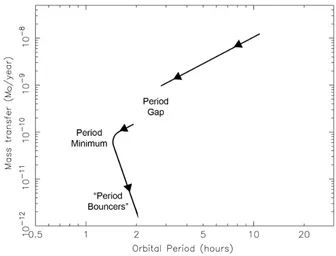
Figure 1-4: Period evolution versus accretion rate. Indicated is the general evolution of a CV from a long period, through the period gap at 2-3 hours, towards the minimum period at around 70 minutes. At this point, more mass transfer results in an increase of the orbital period (Figure based on figure 4.2 from Hellier 2001).
with fMB varying between fMB = 0.73 (Skumanich, 1972) and fMB = 1.78 (Smith,
1979) and k2 = 0.1, the gyration radius of the secondary star (derived from equation 3 of Verbunt & Zwaan 1981). In better understandable units, this amounts to mass loss rates between ˙M ∼10−9−10−8Myr−1 for CVs (Figure1-4).
Gravitational radiation
According to general relativity, matter curves space and the orbital motion of a binary system causes ripples to arise in this space fabric. The energy and angular momentum propagating outwards in these ripples is extracted from the binary orbit, causing the stars to spiral inwards, decreasing the orbital separation and hence the period. This process dominates the period evolution for CVs with orbital periods below 2 hours as magnetic braking is ad hoc disrupted at orbital periods of around 3 hours (Rappaport et al., 1983). General relativity predicts (Landau & Lifshitz, 1975) that the rate of angular momentum loss due to gravitational radiation is given by:
˙
JGR
J =−
32G3
5c5
M1M2M
and results in rates of ˙M ∼10−10M
yr−1 for compact binaries, Figure1-4(Rappaport
et al.,1982).
1.2.4 Mass transfer
We now consider a binary which consists of a WD and a low mass main sequence donor star. To initiate mass transfer (a characteristic of CVs), the secondary star radius must reach its Roche limit. To understand the reaction of the binary on the mass transfer, we need to understand the subtle interplay betweenq, a,M˙ and ˙R2 and on what timescales these processes take place. Three time scales are important for stellar structure and evolution. Firstly, the dynamical time scale on which the star reacts to departures from hydrostatic equilibrium:
tdyn=
r
2R3
GM '40
" R R 3 M M #
minutes. (1-19)
Secondly, the thermal time scale (or Kelvin Helmholtz time scale), which measures the time to react to departures from thermal equilibrium:
tth=
GM2
RL '(3.0×10
7) M M 2 R R L
L years, (1-20)
withLthe luminosity of the star. Hence the donor is always in hydrostatic equilibrium, but not necessarily in thermal equilibrium. The third time scale is the nuclear time scale, which is the characteristic main-sequence lifetime of a star:
tnuc'(7×10⁹)
M
M
L
L years. (1-21)
Transferring mass from the less massive star to the more massive star results in an increase of separation to conserve angular momentum. As the mass ratio also changes, the Roche geometry adjusts to the new system parameters. The change of secondary radius in comparison to this new Roche lobe boundary determines the nature of the mass transfer.
The rate of change of the secondary radius is a combination of the change due to evolutionary changes (on nuclear timescales) and due to mass loss:
˙
R2
R2
= R˙2
R2
!
˙
M2
+ R˙2
R2
!
nuc
. (1-22)
As we can express the radius of a star in terms of its mass using a power law
to mass loss using the logarithmic derivative of the above equation: ˙ R2 R2 ! ˙ M2
=ξ M˙2 M2
!
. (1-24)
For the Roche lobe radius, we can find a similar expression
˙ RL RL ! = 2 ˙ J J !
+ξL
˙
M2
M2
!
. (1-25)
The change in radius can now be expressed solely in terms of the mass loss rate and the two exponents:
˙
R2
R2
− R˙L
RL
' ∆ ˙R
R2
= (ξ−ξL)
˙
M2
M2
(1-26)
with ∆ ˙R= ˙R2−R˙L. As
˙
M2
M2 is negative, ξ−ξL<0 leads to an unstable situation as the stellar radius is always larger than the Roche lobe radius, which leads to an increase in mass loss, and an unstable mass transfer situation. In this situation, the mass transfer rate is on a quicker time scale than the star can contract, the mass transfer will be enhanced, which results in runaway mass transfer (on dynamical or thermal timescales). If ξ−ξL>0, the difference in radius is negative, and the Roche lobe expands with
respect to the stellar radius, which will decrease the mass transfer rate. To maintain stable mass transfer, an additional driving mechanism is needed to keep increasing the difference between the stellar radius and its Roche lobe radius. In CVs this occurs via angular momentum loss via either magnetic breaking or gravitational radiation.
For conservative mass transfer, and the standard situation with ξ = 1, the change in radius depends only the mass ratio of the system asξL= 2q−5/3 (Kolb 2010;Frank et al. 1992). If q & 43, the mass transfer is unstable, and stable mass transfer can only happen in systems with q. 43.
1.2.5 Period distribution
1
2 3
10
100
P
orb(hours)
0
20
40
60
80
100
Number of systems
m
ax
P
orbperiod gap
m
in
P
orb
AM CVns
Evolved secondaries
∼
5
m
in
ut
[image:27.595.129.483.97.367.2]es
Figure 1-5: Period distribution of CVs. Data from Ritter & Kolb (2003). Distinct features are the diminishing numbers with periods above 12 hours, the drop of numbers in the 2-3 hour period range and the sharp cut-off for periods below ∼ 80 minutes. Those systems with orbital periods longer than 12 hours contain an evolved secondary star, and systems with a period shorter than the minimum period contain degenerate, hydrogen deficient components.
In CVs, the orbital period is closely related to the mass and radius of the secondary via
Porb ∝
R32 M2
1/2
(1-27)
hence changes in period can be explained by comparing the change of the radius and mass of the secondary via the exponent ξ.
Maximum orbital period
The maximum period for a CV is set by requiring a slower evolution for the secondary star than for the primary: e.g. q <1, with M1,max =MWD,max<1.4M. A longer
or-bital period gives a larger Roche lobe radius, hence a larger and more massive secondary is needed to establish mass transfer. Using the approximation
hours for M2 ∼ 1.4M. As only few WDs are at the Chandrashekar limit, a smooth
decrease of systems from ∼ 6 hours onwards (equivalent to M2 ∼ 0.6M) is seen in
Figure 1-5.
Period gap
The transition from magnetic braking towards gravitational radiation as the main source for the loss of angular momentum is governed by a change of mass transfer rate, from
˙
M ∼10−9−10−8Myr−1 (magnetic braking) to ˙M ∼10−10Myr−1 (gravitational
ra-diation, Figure1-4). This is not an instantaneous transition, as the secondary’s response to the change of mass is on a longer time scale than the change in mass loss rate occurs. Mass loss results in a drop in weight on the core, this decreases the number of nuclear reactions, dropping the outward pressure and as a result the star contracts. During magnetic braking, this process happens on a long time scale and hence the star is al-ways slightly too large for its mass. When magnetic braking ceases (disruptive magnetic braking, Rappaport et al. 1983) at the upper edge of the gap (observationally deter-mined atPgap,+= 3.18±0.04 hr,Knigge 2006), mass transfer ceases and the secondary can contract to its correct size, detaching from the Roche lobe. Gravitational radiation decreases the period, and the Roche lobes, till at the lower edge of the gap (observation-ally determined at Pgap,−= 2.15±0.03 hr, Knigge 2006), when the secondary and the
Roche lobe come into contact again and mass transfer is resumed. In terms of period changes during both pre- and post-period gap, the mass-radius exponent ξ = 1, which means that R3 decreases quicker than M2, and hence the period will evolve towards shorter periods due to the drive of mass loss via the loss of angular momentum.
Minimum period
After reattachment, the mass transfer will decrease the period until the minimum period, at ∼70 minutes (e.g. Paczy´nski 1971, Kolb & Baraffe 1999, Barker & Kolb 2003) has been reached. This point is defined by the secondary reaching a mass of ∼ 0.08M.
Now the tth exceeds the mass transfer time scale, which is only driven by gravitational radiation, hence the star contacts slower. If R2 decreases more slowly than M
The observationally determined orbital period minimum happens atPmin= 76.2±1.0 minutes (Knigge, 2006), which is close to the theoretically determined value (Pmin ≈ 77min, seeBarker & Kolb 2003 for a discussion).
AM CVn
The AM CVs systems contain two hydrogen deficient, degenerate stars and have very short orbital periods (below the period minimum) while sustaining mass transfer via
rlof. There are three proposed routes for the formation of an AM CVn system. The
first route has an initial system containing two WDs, with gravitational radiation short-ening the period until mass transfer starts at which point the system will evolve towards longer periods. The second route contains a low mass, non-degenerate helium star transferring mass onto a WD. At a period of∼10minutes, the helium star will become semi-degenerate and the period will increase with further mass loss. The last route states that the AM CVn is born from a CV containing an evolved secondary star which uncovers a He-rich core after mass loss, causing the period to increase. For a recent review of these evolution channels, see Solheim (2010).
Evolved secondaries
Several systems exist with an orbital period above ∼ 12 hours. These contain a sec-ondary star evolving towards the red giant phase (low density). As the secsec-ondary is expanding in these systems, independently of mass loss, the orbital period will evolve towards even longer periods.
1.3
Dwarf Novae
Figure 1-6: Top: Lightcurve of Z Cam, the prototype system of those DNe that show prolonged standstills. Middle: Lightcurve of the SU UMa type DN VW Hyi showing both regular and superoutbursts. Bottom: Lightcurve of the WZ Sge type system GW Lib during its most recent superoutburst in 2007. Note the difference in magnitude scaling. Constructed from observations made by the AASVO.
• Z Camsystems show prolonged standstills at∼0.7 mag below maximum
bright-ness as the outburst ceases for periods of days to years (top panel, Figure1-6).
• SU UMahave occasional super-outbursts. These bursts achieve a brighter state (by∼0.7 mag) and remain in outburst for∼5 times longer than normal outbursts (middle panel, Figure 1-6).
– WZ Sge type systems are a sub-class of the SU UMa type, but are char-acterised by having short orbital periods and very low accretion rates (∼
10−11Myr−1) resulting in the display of only very rare but extremely bright
outbursts on recurrence time scales of 10-20 years (bottom panel Figure1-6).
• U Gemsystems are those DNe that neither show standstills nor super-outbursts.
1.3.1 Disc outburst
The sudden brightening of CVs are associated with an increase in luminosity arising from the accretion disc. However, steady state accretion flows cannot describe time-dependent phenomena such as these semi-regular outbursts. Osaki (1974) and H¯oshi
height H and local sound speed cs, the viscosity can be expressed in terms of the α
-parameter: ν =αcsH withα.1 (Shakura & Sunyaev,1973). Due to the long viscous
time scale, mass transfer through the disc onto the WD, is slower than mass transfer into the disc from the donor, and hence material accumulates. At the onset of the outburst, the disc will become unstable, increasing the viscosity and the transport of material both inwards and outwards, increasing the size of the disc as well as the accretion rate of material onto the WD. This increase in accretion and viscosity enhances the luminosity of the system and drains the material from the disc. Once drained, the disc will return to its low-viscosity, low-luminosity state. After outburst, interaction between the mass transfer stream and the disc will decrease the disc size as in-falling material has angular momentum corresponding to the circularisation radius and this cycle can then repeat itself.
Disc instability
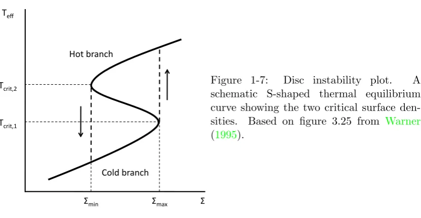
The disc instability model for DNe is based on the limit-cycle between the effective temperature (Teff) and the surface density (Σ) for an annulus of the disc at radius R. The turning points on the equilibrium curve between the surface density and the effective temperature (and indirectly mass transfer rate) of a disc annulus, are defined by Σminat
Tcrit,2, ˙Mcrit,2 and by ΣmaxatTcrit,1, ˙Mcrit,1, withTcrit,1< Tcrit,2and ˙Mcrit,1<M˙crit,2, see Figure 1-7. The curve indicates thermal equilibrium, that is, when the viscous heating balances the radiation from the surface. Any annulus with Σ, T to the right of the curve will heat up as the heating exceeds the cooling and move upwards in the diagram till it reaches the top of the S-curve. Whereas an annulus with Σ, T to the left of the curve will cool down till it reaches equilibrium on the lower branch of the curve.
Stable configurations are on those branches when dTeff/dΣ > 0, while the branch with dTeff/dΣ<0 is unstable. A positive perturbation on this branch causes Σ to rise and hence a larger T is needed which causes a movement away from the curve. For a negative perturbation, Σ decreases, which requires a cooler T.
The cycle between quiescence and outburst in DNe can be seen as a cycle through the curve. During quiescence an annulus of the disc lies on the lower branch but with
˙
!"#$%&'()*+% ,"-%&'()*+%
.%
./0)% ./(1%
2*'0-56%
[image:32.595.110.526.76.292.2]2*'0-57%
Figure 1-7: Disc instability plot. A schematic S-shaped thermal equilibrium curve showing the two critical surface den-sities. Based on figure 3.25 from Warner
(1995).
the S-curve. As now, ˙M <M˙crit,2, the surface density decreases until it reaches the left turning point. Decreasing Σ further results in a cooling of the ring towards the lower branch.
An outburst in the disc of a DN is initiated in the annulus which is first pushed over its critical surface density. This causes instability in the neighbouring annuli, sending heat waves through the disc until most of the disc is on the upper branch. The reverse happens for the return to quiescence, as cooling waves propagate through the disc once an annulus returns to the lower branch.
1.3.2 Superhumps
During super-outbursts, low mass ratio DNe show large amplitude variations in their light curves at periods slightly longer than the orbital period of the system, see Figure 1-8 for the September 2007 superoutburst of V455 And. These are called superhumps after the super orbital humps in the light curve.
Theory
Figure 1-8: Lightcurve of the 2007 superoutburst of V455 And. The insets show a close up of the curve during the plateau phase (bottom left) and the general decline (top right), displaying the superhumps: variations in the brightness of around one magnitude, and with a period slightly longer than the orbital period. Constructed from observations made by AASVO.
1997;Simpson & Wood 1998;Wood et al. 2000). These studies also find a critical mass ratio at which superhumps cease to happen, qcrit ∼0.3, this limit is mainly set by the maximum mass ratio in which the 3:1 tidal interaction point is still placed inside the maximum extent of the disc.
Smoothed particle hydrodynamics (sph) is a Lagrangian method, which models the
flow of a fluid as a set of moving particles (Monaghan,1992). Sphsimulations byMurray
(1998) show that the energy released from a disc that has become tidally unstable is suf-ficient to account for the excess luminosity of a superoutburst, and produces superhumps in the integrated light curve of the disc. Foulkes et al.(2004) show 2-Dsphsimulations
for a system with q = 0.01 that reveal an eccentric, non-axisymmetric precessing disc of changing density, which is continuously stretching and relaxing on the superhump period. Figure1-9shows the surface density maps, which display tightly wrapped spiral density waves that extend from the outermost regions to small radii. These produce shear and dissipation in the outer disc, and propagate angular momentum outwards, allowing disc gas to move inward.
Lubow (1991a,1991b, 1992) shows that the final precession rateω for an eccentric disc can be split into three terms:
−0.6 −0.4 −0.2 0 0.2 0.4 d
Normalized binary separation y
−
direction
−0.6−0.4 −0.2 0 0.2 0.4 0.6
−0.6 −0.4 −0.2 0 0.2 0.4 0.6 g
Y Velocity (km/s)
−1000 −500 0
−500 0 500
0.6 0.4 0.2 0 0.2 0.4 0.6e
Normalized binary separation x−direction
−0.6−0.4−0.2 0 0.2 0.4 0.6
h
X Velocity (km/s)
−1000 −500 0
0.6 0.4 0.2 0 0.2 0.4 0.6f
−0.6−0.4−0.2 0 0.2 0.4 0.6
i
G H
[image:34.595.123.501.70.336.2]−1000 −500 0
Figure 1. The top row (a, b, c) shows accretion disc surface density maps using a logarithmic colour-scale for binary phases 0.00, 0.36, and 0.64, respectively. The secondary orbits anticlockwise with respect to the inertial frame, with mass being added from theL1point at the right of each map. The solid curve is the Roche lobe of the primary, plotted in a frame that corotates with the binary. The arrow in the lower right-hand corner of each map indicates afixed direction to an observer. The middle row (d, e, f) shows the corresponding dissipation maps plotted with a logarithmic colour-scale. The bottom row (g, h, i) shows the matching Doppler maps plotted using a linear colour-scale. The letter‘G’on map (i) indicates the point at which the gas stream impacts on the outer edge of the accretion disc and the letter‘H’indicates the arc of emission produced by the disc particles in the impact region.
superhumps are invariably detected in optical light. Because the hot inner regions of a viscously heated disc contribute relatively little to the total optical light, the comparison between observation and our simulation might best be made by comparing one of the lower curves in Fig. 2.
Fig. 1(d) corresponds to the light curve minimum. From this map it is clear that the dissipation at the stream–disc impact is at a min-imum. This is because the spiral compression arm in the outer disc has moved such that gas is escaping from the primary Roche lobe and returning to the secondary. The gas leaving theL1point from
the secondary encounters the disc gas instantly and the twoflows have a low relative velocity. Hence, relatively little dissipation is generated by the convergingflows. At this phase the dissipation is dominated by the shearflow in the inner regions of the disc.
As the binary orbit proceeds, a large void opens up between the
L1point and the accretion disc, as shown in Figs 1(b) and (e), and
the spiral arm which previously extended towards the L1region
becomes detached from the disc under centrifugal forces and then falls back towards the disc. When this gas hits the disc, the im-pact causes a sudden rise in dissipation, corresponding to the spiky
C
!2004 RAS, MNRAS349,1179–1192 Figure 1-9: Example of sph simulations. Top: (a, b, c) shows accretion disc surface
density maps using a logarithmic colour-scale for binary phases 0.00, 0.36, and 0.64, respectively. The secondary orbits anticlockwise with respect to the inertial frame, with mass being added from the L 1 point at the right of each map. The solid curve is the Roche lobe of the primary, plotted in a frame that co-rotates with the binary. The arrow in the lower right-hand corner of each map indicates a fixed direction to an observer. The bottom row (d, e, f) shows the corresponding dissipation maps plotted with a logarithmic colour-scale. Figure 1 fromFoulkes et al.(2004).
where ωdyn is the dynamical precession frequency arising from the resonance, ωpress is a pressure-related term acting to slow the precession and ωtran is a transient term. This latter contribution is related to the time-derivative of the mode giving rise to the dynamical precession.
Observations
Observers express the amount of precession as the fractional difference between the observed superhump period and the orbital period:
= Psh−Porb
Porb
. (1-30)
For ωpress,dyn ωorb, this can be expressed in precession terms, and hence linked to theory, via:
0.04
0.06 0.08 0.1
0.2
P
orb(days)
10
-210
-1²
=
(
P
sh−
P
orb
)
/P
orb
Observed
P
orb−²
relation
0.1
0.2
0.3
q
=
M
2/M
1²
−q
calibrators
0.00
0.01
0.02
0.03
0.04
0.05
0.06
0.07
0.08
Figure 1-10: Left: Porb versus the superhump period excess (based on data from
Ritter & Kolb 2003. Theblack stars indicate those systems that are part of the survey conducted in this thesis. The black line indicates the predicted trend for the mass loss rate if the angular momentum loss is solely governed by gravitational radiation (data from Kolb & Baraffe 1999). Right: Mass ratio q versus the superhump period excess, note the differently scaled y-axis. The black dots are Patterson’s calibrators. The lines represent the different relations: Patterson’s empirical relation (dotted line;
2005), Knigge’s relation (solid;2006) and Kato’s relation (dashed;2009). Also indicated in respectively black diamondand black starare theLMXBKV UMa and the eclipsing
AM CVn system SDSS J0926+3624.
(equation 25,Pearson 2006). Figure1-10shows the orbital period versus observed super-hump excess for all CVs in the catalogue ofRitter & Kolb(2003). The red line indicates the predicted period evolution if the angular momentum loss is solely governed by grav-itational radiation and an assumed empirical relation of (q), which underestimates the mass loss rate. A better fit is found when assuming ˙J ∼3 ˙JGR (Townsley & Bildsten,
2003).
Several observational studies have been carried out to find a relation between super-hump period and the system parameters of the binary. To date, the best determined relation is found between the mass ratio and the superhump excess (Patterson et al.,
2005), following the theoretical prediction by Mineshige et al. (1992) of= 0.34q. Based on twelve systems (10 eclipsing systems, 1 assumed upper limit to the period and one eclipsing Low Mass X-ray binary (lmxb) with an extremely low mass ratio; see table 7, Patterson et al. 2005) they fix the relation to:
= 0.18q+ 0.29q2 (1-32)
Figure 1-11: Comparison of the calibration systems from Patter-son et al. (2005) with a model with purely dynamical precession (solid) and including the pressure term (dashed; figure 5 from Pear-son 2006).
parameters of Patterson’s calibrators with no fixed origin assumptions:
q() = (0.114±0.005) + (3.97±0.41)×(−0.025). (1-33)
A final relation is presented by Kato et al. (2009) based on a large scale observational campaign of superhumping CVs:
= 0.16q+ 0.25q2. (1-34)
All these relations and the initial set of calibrator systems are plotted in Figure1-10. The tie between observations and theory is investigated byPearson(2006). He shows that the pressure term is needed to fit the list of (q) calibrators as given by Patterson et al.(2005), see Figure1-11. His best relation is derived from theory, by generating(q) predictions from the formula numerically and then finding the best-fitting polynomial to these values:
= 3.5×10⁻⁴+ 0.24q−0.12q2 (1-35) and is valid for 0.01< q <0.4.
1.4
Setting the scene
Theory predicts that a large fraction (roughly 70%) of CVs should have passed through the minimum period. The Sloan Digital Sky Survey (sdss) sample is finally unearthing
G¨ansicke et al. 2009). But due to their faint donor stars, the orbital period is often the only measurable system parameter for most candidate post-period minimum CVs. The indirect measurable of the superhump period, and hence superhump excess could potentially provide an indication of the mass ratio of the systems via the empirical re-lation between the two observables. While this rere-lation is potentially very useful for the determination of mass ratios, the large scatter in the calibrators, especially at the low mass ratio end, prohibits a direct conversion between easy to measure light curve variability and the much sought after mass ratio.
To place a short period CV firmly on the evolutionary track (e.g pre- or post bounce), more direct methods to determine the mass ratio are required. But also a better cali-bration and validation of this above relation is needed. In this thesis, we will explore new emission line diagnostics for accreting compact objects using traditional emission line features and the more ‘exotic’ calcium ii lines in the I-band. The direct aim is to
Methods
CVs display spectral features originating from a range of system components. The typical temperatures of the components results that CVs are good sources over a range of wavelengths, from X-ray and UV to optical to infra-red (IR). This, combined with their relative brightness and short orbital periods, makes CVs excellent objects to pursue with time-resolved optical spectroscopy. Studying the spectral features from the different components throughout the orbital period provides us with measures for their radial velocities (K1 and K2) which dynamically constrain the system parameters (e.g. q =
K1/K2). These are of extreme importance for binary evolution tests, as we saw in Chapter 1.
For this thesis, we acquired a considerable amount of time-resolved spectroscopic data. This Chapter covers the reduction and analysis steps we followed for all observed CVs.
2.1
Spectral features in CVs
White Dwarf
A hydrogen dominated WD (type DA) spectrum shows mainly broad Balmer absorption lines due to the high pressure in its atmosphere. The shape of these lines is a direct function of the temperature and logg, and can be used to determine these parameters in single WDs. In accreting WDs, narrow metal lines from freshly accreted gas can be seen in absorption. As the WD is heated by accretion, temperatures are generally
&10 000K, thus their continuum emission peaks in the blue (Figure 2-1). In a binary, the radial velocity curve of the WD as a function of the orbital period gives K1.
Donor star
Fig. 3: The principal components of a cataclysmic variable spanning the X-SHOOTER range. Fluxes are scaled to a nominal system at 10pc and show the contributions from the accreting white dwarf (solid curve: T=15,000 K) dominating at short wavelengths, the accretion flow (dashed curve: optical thin continuum model appropriate for low mass transfer rates) and the mass donor star. Shown is a sequence of late-type donors scaled to their approximate contribution to the SED going from M to L type (spectra from the Cushings et al. (2005) and Hawley et al. (2002) atlases). It is the unrivalled simultaneous coverage across such a broad range that makes X-SHOOTER an exquisite instrument for this purpose. Depending on the type and brightness of the donor star, a large number of spectral segments offer opportunities for detecting donor star features while the blue end anchors the WD and accretion contributions. Good spectral resolution is needed to avoid diluting sharp features (such as those around 1.1-1.3µ) as well as provide an acurate trace ofK2andvsiniof the donor.
5
-Figure 2-1: Spectrum displaying the principal components of a cataclysmic variable. Fluxes are scaled to a nominal system at 10pc and show the contributions from the accreting white dwarf (solid curve: T = 15 000K) dominating at short wavelengths, the accretion disc (dashed curve: optically thin continuum model appropriate for low mass transfer rates) and the donor star. Shown is a sequence of late-type donors scaled to their approximate contribution to the SED going from M to L type (spectra from the
Cushing et al. (2005) andHawley et al. (2002) atlases). Courtesy Tom Marsh.
Single low mass, main sequence stars display spectral features due to absorption by a broad range of metals at these wavelengths. In CVs, these absorption features can be suppressed by irradiation on the inner hemisphere of the donor, and hence are primarily visible on the cool backside of the donor. When present, we can use these lines to determine the projected radial velocity (Kabs & K2). However, in DNe systems the donor stars are faint compared to the accretion disc continuum and direct detection of these absorption lines is often very difficult, in the optical range.
Irradiation of the inner hemisphere of the donor can give rise to emission lines if enough energy is available to excite hydrogen and helium. This is normally only the case just after a disc outburst. The emission will have a radial velocity ofKem ≤K2 as only the front is irradiated.
Accretion Disc
As the temperature in the accretion disc is dependent on the radius (equation 5.43,
[image:39.595.167.465.87.310.2]A B
Figure 2-2: Double peaked profile (B) formation from the accretion disc (A). Regions of constant radial velocity in the disc are shown as hatched areas on the left. The corresponding velocity bins are indicated by the same hatched pattern, in the line profile on the right. Figure fromHorne & Marsh (1986).
must be seen as the sum of black bodies with temperatures appropriate for each radius in the disc. For discs around CVs, the emission peaks in the UV and optical as the disc is constrained in size (Figure 2-1). The overall luminosity is set by the accretion rate, and in high rate cases the luminous disc can obscure both the donor and WD features. The accretion disc in quiescent DNe is optically thin and reveals itself as double peaked hydrogen emission lines due to the range of velocities in the rotating disc and their projection along our line of sight (Figure2-2). In outburst, the disc manifests itself as a more luminous continuum as it transforms into a hot, optically thick disc and the spectral features can become dominated by strong and single peaked absorption lines. However, some optically thick discs display emission line regions as well and hence the line profiles from the disc are not always a clear indication of the state of the disc. By tracing the radial velocity of the disc (Kdisc) we can indirectly trace K1, as the disc is centred on the WD and thus should track its radial velocity curve.
Total DNe spectrum
spectrum and allow K1 and K2 to be measured. Unfortunately, the donor becomes intrinsically faint just at those short periods when the mass accretion rate decreases.
2.2
Time-resolved spectroscopy
2.2.1 Spectroscopy
Using a spectrograph, the light emitted by a source can be dispersed as a function of wavelength. Using a long-slit at the focus of the collimator, the parallel light rays from a distant star are directed as a parallel beam towards a diffraction grating (either transmissive or reflective). The grating diffracts wavelengths at different angles, per-pendicular to the slit direction. Finally, the camera focuses all light travelling at any given angle onto a unique point on the detector.
The resolving power of the spectrograph is normally quoted as R=λ/∆λ, with ∆λ
the smallest difference in wavelength to be measurable at a wavelengthλ(e.g. vlt/uves
has a resolving power ofR∼80 000, whereaswht/isishasR∼800−7000). The actual
resolution is a function of the number of lines on the diffraction grating, and the width of the slit and order, as a narrower slit can provide a higher resolution as can using a higher order, but both at the cost of loss of light.
The wavelength range of the observed spectrum is dependent on the diffraction grating, angle, size of the Charge-Coupled Device (ccd, Boyle & Smith 1970) and the
observed order, hence a wavelength calibration is required for every set-up change. A flux calibration is also needed along the wavelength axis, as the optics throughput and the response of the detector are wavelength dependent.
CVs have orbital periods between 80 minutes and several hours. Sampling the orbit and measuring the shifts of the lines as a function of time, provides measures of the period, phase and velocity semi amplitude of the components. On one hand, a maximum exposure time is set by our wish to minimise smearing and broadening of features. The amount of smearing depends on the K-amplitude of the line features as the radial velocity changes during the exposure, and long exposures naturally broaden all features. On the other hand, the minimum exposure time is set by the requirement of a S/N>6 to avoid read out noise domination on theccdused for astronomical observations in the
Figure 2-3: Top to bottom: Raw data frame for UV Per (WHT August 2009 run) showing both the object spectrum along the x-direction as well as the spectrum of a nearby reference star. Also visible are the multiple sky lines present in this wavelength range (vertical lines) and cosmic rays (white dots). After bias and flat field correction and optimal extraction of the spectrum along the dispersion direction, the second panel shows the reduced spectrum of UV Per. The bottom panel shows the final product: a normalised and wavelength calibrated spectrum.
2.2.2 Data reduction
ccd data requires a set of calibrations to reduce the raw 2-D images (Figure 2-3, top panel) into 1-D spectra (bottom panel). The three sources of noise contributing to accd
image are the read out noise, the thermal noise and the fixed pattern noise. To correct for these features bias, dark and flat field frames are needed. This is followed by the extraction of the spectra and, finally, the conversion from ccd-pixels into wavelength
units and fromccd-counts into flux units.
Bias correction
Read out noise (ron) is introduced by the error in the charge measurement process and
pixel after read out (as the storage of the sign requires an extra data bit) a bias level of order 100 - 1000 electrons is added to each pixel. We can correct for this level in two ways. The first way is to add an ‘overscan’ region on each frame. These pseudo-pixels are not exposed to light and can be averaged to find the bias level andronof the frame
in question. The second method is to obtain frames with a zero exposure time and the shutter closed to avoid incident light. To reveal any static 2-D bias structure, these frames are stacked, averaged and subtracted from each science frame. For this work, the 2-dimensional bias frames are first median stacked and then subtracted. Any remaining small deviations are corrected for using the overscan region.
Dark correction
Thermal excitation of electrons give rise to an additional source of noise in the frame which builds up over time. To correct for this effect one can take dark frames, which are frames with the same exposure time and settings as the science frame but with the shutter closed. However, most modern detectors have a negligible dark current when cooled with liquid nitrogen to reduce the thermal excitation, a method commonly used at telescopes as it makes dark frames redundant, reducing overhead times. All data taken for this work comes from such cooled ccds, voiding dark current correction.
Flat field correction
The fixed pattern noise, or pixel-to-pixel variation of theccdcan be corrected for with
flat fields. Uniformly illuminating the ccd using bright, featureless lamps reveals the
response of the individual pixels. This includes small variations of up to 1% but also the more problematic features like non-responsive (or dead) pixels. Again, several frames are averaged to find the static flat field. For spectroscopy, the flat fields are not flat as the spectral shape of any flat field source is dependent on the wavelength. Hence, the science frames are not divided directly by the flat field, as is done in photometry, but by a frame that is created by fitting the flat field shape along the wavelength axis and dividing the flat field by this. The result is a normalised 2-D image with variations of up to a few percent which all science frames are divided by.
Both the bias and flat field corrections for spectroscopy in this work are done using thestarlink package figaro1. I have written several C-shell scripts to automate the
1
Spectral extraction
The optimal extraction method, as presented by Marsh (1989), is commonly used for the extraction of distorted and tilted spectra. The extraction procedure is a succession of several (dependent) steps, and assumes that the image of the slit lies roughly parallel to the rows of the ccdand the dispersion is roughly parallel to the columns. The first
step is fitting a low order polynomial to the spectrum along the dispersion direction to track curvature and tilt introduced by the spectrograph optics. On a line perpendicular to this track, a low order polynomial is fitted to sky background regions. For the object region a profile is fitted, again perpendicular to the track, to calculate the contributing pixels and their weight. In a final step both the background subtraction is performed as well as the final extraction of the spectrum using the optimal weights estimated in the previous steps, while cosmic outliers are identified and removed. The final product is a 1-D spectrum in pixels versus counts (Figure 2-3, middle panel).
We controlled the spectral extraction using the 2-D spectral reduction suite Pamela,
provided by Tom Marsh, via custom scripts, using C-shell and Python.
Wavelength calibration