Conical diffraction intensity profiles generated using a top hat input beam

Conical diffraction intensity profiles

generated using a top-hat input beam

R. T. Darcy,∗D. McCloskey, K. E. Ballantine, J. G. Lunney, P. R. Eastham, and J. F. Donegan

AMBER & CRANN, School of Physics, Trinity College Dublin, Ireland ∗_{[email protected]}

Abstract: The phenomenon of internal conical diffraction has been studied extensively for the case of laser beams with Gaussian intensity profiles incident along an optic axis of a biaxial material. This work presents experimental images for a top-hat input beam and offers a theoretical model which successfully describes the conically diffracted intensity profile, which is observed to differ qualitatively from the Gaussian case. The far-field evolution of the beam is predicted to be particularly interesting with a very intricate structure, and this is confirmed experimentally.

© 2014 Optical Society of America

OCIS codes: (260.1180) Crystal optics; (050.1940) Diffraction.

References and links

1. W. R. Hamilton, “Third supplement to an essay on the theory of systems of rays,” Trans. R. Irish Acad. 17, 137–139 (1837).

2. A. M. Belsky and A. P. Khapalyuk, “Internal conical refraction of bounded light beams in biaxial crystals,” Opt. Spectrosc. 44, 746–751 (1978).

3. M. V. Berry, “Conical diffraction asymptotics: fine structure of the Poggendorff rings and axial spike,” J. Opt. A, Pure Appl. Opt. 6(4), 289–300 (2004).

4. M. V. Berry, M. R. Jeffrey, and J. G. Lunney, “Conical diffraction: observations and theory,” Proc. R. Soc. A 462, 1629–1642 (2006).

5. C. F. Phelan, D. P. O’Dwyer, Y. P. Rakovich, J. F. Donegan, and J. G. Lunney, “Conical diffraction and Bessel beam formation with a high optical quality biaxial crystal,” Opt. Express 17(15), 12891–12899 (2009). 6. C. F. Phelan, K. E. Ballantine, P. R. Eastham, J. F. Donegan, and J. G. Lunney, “Conical diffraction of a Gaussian

beam with a two crystal cascade,” Opt. Express 20(12), 13201–13207 (2012).

7. D. P. O’Dwyer, C. F. Phelan, Y. P. Rakovich, P. R. Eastham, J. G. Lunney, and J. F. Donegan, “The creation and annihilation of optical vortices using cascade conical diffraction,” Opt. Express 19(3), 2580–2588 (2011). 8. R. T. Darcy, D. McCloskey, K. E. Ballantine, B. D. Jennings, J. G. Lunney, P. R. Eastham, and J. F. Donegan,

“White light conical diffraction,” Opt. Express 21(17), 20394–20403 (2013).

9. D. P. O’Dwyer, C. F. Phelan, K. E. Ballantine, Y. P. Rakovich, J. G. Lunney, and J. F. Donegan, “Conical diffrac-tion of linearly polarised light controls the angular posidiffrac-tion of a microscopic object,” Opt. Express 18(26), 27319–27326 (2010).

10. A. Turpin, V. Shvedov, C. Hnatovsky, Y. V. Loiko, J. Mompart, and W. Krolikowski, “Optical vault: A reconfig-urable bottle beam based on conical refraction of light,” Opt. Express 21(22), 26335–26340 (2013).

11. M. Born and E. Wolf, Principles of Optics (Cambridge University, 1999).

12. L. D. Landau, E. M. Lifshitz, and L. P. Pitaevskii, Electrodynamics of Continuous Media (Pergamon, 1984). 13. M. V. Berry and M. R.Jeffrey, “Hamilton’s diabolical point at the heart of crystal optics,” Prog. Opt. 50, 13–50

(2007).

14. M. C. Pujol, M. Rico, C. Zaldo, R. Sol´e, V. Nikolov, X. Solans, M. Aguil´o, and F. D´ıaz, “Crystalline structure and optical spectroscopy of Er3+-doped KGd(WO4)2single crystals,” Appl. Phys. B 68, 187–197 (1999). 15. M. R. Jeffrey, Conical Diffraction: Complexifying Hamilton’s Diabolical Legacy (University of Bristol, 2007). 16. V. Peet, “The far-field structure of Gaussian light beams transformed by internal conical refraction in a biaxial

crystal,” Opt. Commun. 311, 150–155 (2013).

18. A. Ashkin, Optical Trapping and Manipulation of Neutral Particles Using Lasers (World Scientific, 2007). 19. M. V. Berry, “Conical diffraction from an N-crystal cascade,” J. Opt. 12, 75704–75712 (2010).

20. T. A. King, W. Hogervorst, N. S. Kazak, N. A. Khilo, and A. A. Ryzhevich, “Formation of higher-order Bessel light beams in biaxial crystals,” Opt. Commun. 187, 407–414 (2001).

1. Introduction

Conical diffraction was first predicted by William Rowan Hamilton of Trinity College Dublin in 1882 [1]. As part of his extensive work on mathematical optics, he predicted that a light ray incident along an optic axis of a biaxial medium would be transformed into a hollow cone of light inside the material. If the material was cut such that the entrance and exit faces were parallel to each other and orthogonal to an optic axis, then the light would emerge as a hol-low cylinder. This prediction was experimentally confirmed later that year by Humphrey Lloyd using the biaxial material arragonite. Hamilton’s consideration was that of a refractive phe-nomenon and led to the term ‘conical refraction’. It was not until the development of the theory by Belsky and Khapalyuk [2], which considered diffraction in a paraxial wave-theory model, that the nomenclature was switched to ‘conical diffraction’. This model was later reformulated by Berry [3] and remains a highly accurate description of the phenomenon; notably present in the model is the Poggendorff dark ring, a narrow region of zero intensity between two bright rings, which is absent from Hamilton’s treatment. It is for this reason that we will refer to the phenomenon as ‘conical diffraction’.

Conical diffraction has been extensively studied using an input laser beam [4–7]. Such beams are approximately Gaussian, and so the models describing conical diffraction often assume an input Gaussian beam. Even in cases where broad sources were used to produce the phe-nomenon, it was important to use a spatial filter to form a spatially coherent beam which was approximately Gaussian in the focal image plane in order for the established theory to remain valid [8]. In this paper we consider another type of input beam, namely a ‘top-hat’ beam, and demonstrate how it exhibits interesting intensity profiles beyond the crystal with a rich beam evolution structure. Although the first observation of conical diffraction by Lloyd used a pinhole in front of arragonite, thus resulting in a top-hat beam, since then it appears no experimental im-ages have been produced with this beam profile. We present experimental imim-ages of conically diffracted beams produced using a top-hat source which are qualitatively different from those produced using a Gaussian source, in particular featuring a narrow ring of high intensity and a wedge-shaped structure with a rapid drop in intensity at the beam edge. This novel and unusual beam shape could find applications in areas such as optical trapping [9, 10], laser etching, and high NA direct write photolithography.

2. Theory

Conical diffraction is an optical phenomenon observed in biaxial materials, which have three principal refractive indices n1<n2<n3. Light incident along one of the two optic axes in such a material undergoes internal conical diffraction and spreads out as a hollow cone with semi angle

A=1₂arctan

n2₂n−2₁ −n−2₂ n−2₂ −n−2₃ . (1)

The geometrical optics description of this may be found in [11] and [12]. For many biaxial materials A is small, on the order of 10−2rad, and hence a paraxial approximation may be used to determine the radius of the ring of light as it emerges from such a material of length l:

R0= l

2

sin(2A) cos(2A)=

l

A rigorous examination of the validity of this paraxial approximation when modelling conical diffraction is shown in [13]. The biaxial material used in the experiments presented in this paper is KGd(WO4)2whose principal refractive indices have been determined by Pujol et al. [14]. For light at 632.8 nm the values are calculated to be n1=2.0109, n2=2.0414, and n3=2.0950.

In order to develop a theory which describes conical diffraction it is useful to first define some dimensionless beam parameters following the notation used by Berry and Jeffrey [13]:

ρ0≡Al

w =

R0

w, ρ≡

R

w, ζ≡

l+ (z−l)n2 n2k0w2 =

Z n2k0w2,

(3)

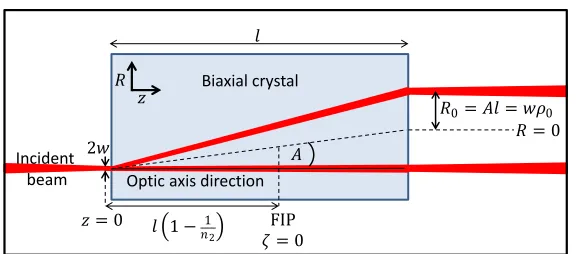
where k0=2π/λ, R is measured along the radius of the beam with R=0 at the centre of the beam, and z is measured along the propagation direction of the beam with z=0 at the location of the focused image of the source in the absence of the crystal. The terms in these equations may be seen in Fig. 1. While these parameters are defined for Gaussian beams with a 1/e

intensity radius of w, they are also useful for top-hat beams where w has been defined to be the radius of the beam. Whenζ=0 the conically diffracted rings are most sharply defined and this location is known as the focal image plane (FIP). Lettingζ =0 in Eq. (3) yields the location

zFIPof the FIP measured from z=0:

zFIP=l(1−1/n2). (4)

FIP = 0 2

1− 1₂ Optic axis direction

Biaxial crystal

Incident beam

= 0

0= = 0

= 0

Fig. 1. A light beam undergoing conical diffraction within a biaxial material. This diagram is a two-dimensional slice taken along the plane where R=0.

When a beam with electric displacement field profile D0(ρ)enters a biaxial material along the optic axis it is conically diffracted. If the beam is radially symmetric and circularly polarised (or unpolarised), the equations describing this transformation are [3]

B0(ρ,ρ0,ζ) = _∞

0

dκ κa(κ)exp−1₂iζκ2J0(κρ)cos(κρ0), (5)

B1(ρ,ρ0,ζ) = ∞

0

dκ κa(κ)exp−1₂iζκ2J1(κρ)sin(κρ0), (6)

where J_ν(x)is theνthorder Bessel function of the first kind and a(κ)is the Fourier transform of the input profile D0(ρ)given by

a(κ) = _∞

0

The intensity distribution after the crystal is then given by [3]

I(ρ,ρ0,ζ) =|B0(ρ,ρ0,ζ)|2+|B1(ρ,ρ0,ζ)|2. (8)

The electric displacement field profile of a Gaussian beam can be expressed, in terms of the beam parameters shown in Eq. (3), as

D0G(ρ) =exp

−ρ2_{/2. (9)}

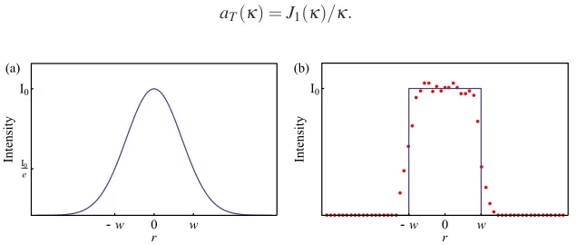
The corresponding intensity profile is plotted in Fig. 2(a). Using Eq. (7) the Fourier transform of a Gaussian beam is

aG(κ) =exp

−κ2_{/2. (10)}

Top-hat beam electric displacement field profiles are given by

D0T(ρ) =Θ(1−ρ), (11)

whereΘ(x)is the unit step function defined by

Θ(x)≡

0, x<0

1, x≥0. (12)

The top-hat intensity profile is plotted in Fig. 2(b). The corresponding Fourier transform of a top-hat beam is then obtained using Eq. (7):

aT(κ) =J1(κ)/κ. (13)

(a) (b)

-w 0 w

I0 e I0

r

Intensity

-w 0 w

I0

r

Intensity

Fig. 2. Plot (a) is a Gaussian intensity profile calculated using the electric displacement field given by Eq. (9). The value w is the 1/e radius of the beam. Plot (b) shows a top-hat profile calculated using the electric displacement field given by Eq. (11). The red dots in (b) show a profile, taken from an experimental image, of the beam used in the experiments which demonstrates a reasonably good approximation of a top-hat beam.

ρ/ρ0 ρ/ρ0

0 0.25 0.5 0.75 1 1.25 1.5 0 0.25 0.5 0.75 1 1.25 1.5

Intensity (arb. units) Intensity (arb. units)

(a) (b)

Fig. 3. Intensity profiles at the FIP generated using Eq. (8) in the case of (a) a Gaussian input beam, as given by Eq. (9), and (b) a top-hat input beam, as given by Eq. (11).

3. Fine structure of the radial intensity profile at the FIP

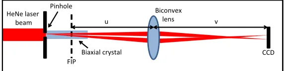
The intriguing intensity profile predicted to occur for a top-hat input beam as seen in Fig. 3(b) merits closer examination. The singularity cannot of course be infinite in reality, but what we actually observe is still of interest and should be quantified. In order to study this profile in fine detail the experimental apparatus shown in Fig. 4 was used. A Helium-Neon (HeNe) laser beam with a peak emission at 632.8 nm was directed onto a 100µm diameter pinhole. Since the radius of the laser beam was of the order of millimetres, the 100µm pinhole acted to cut off enough of the beam to generate a top-hat profile. A 22 mm long slab of KGd(WO4)2was placed as close as possible to the pinhole and the crystal was aligned so that the beam propagated along an optic axis. A biconvex lens of focal length f =3 cm was placed u=3.11 cm after the FIP whereζ =0. This location occurs inside the crystal as can be found using Eq. (4). The image of the FIP was formed 86 cm after the lens, where a colour charge-coupled device (CCD) of pixel size 4.65µm was placed to record the profiles generated. The magnification produced by the lens was calculated to be m=|v/u|=28 which was sufficient to almost fill the CCD chip with the entire singularity and wedge structure. The unmagnified FIP radius was determined to be R0=360±10µm which corresponds toρ0=7.2 when using a pinhole with a 50µm radius. Note that this value differs from the predicted value of R0=430µm obtained using Eq. (2), a discrepancy which is discussed in more detail in [8].

FIP

CCD Biconvex

lens HeNe laser

beam

Pinhole

v u

Biaxial crystal

Fig. 4. The experimental setup used to study the fine structure of the beam profile in the FIP which is imaged onto the CCD. The values of u and v can be adjusted independently to give the image a desired magnification.

An example of the images recorded using this apparatus is shown in Fig. 5. Both images are taken at the FIP, with Fig. 5(b) demonstrating the observed profile when using a top-hat input beam. Figure 5(a) is an image generated using a Gaussian input beam as reported by Darcy et

(a) (b)

Fig. 5. (a) An experimental image of the conically diffracted Gaussian beam in the FIP. The structure is distinct from that formed when using a top-hat input beam as seen in (b). The radius of the Poggendorff dark ring in image (b) was determined to be 360±10µm. Both images are 0.8 mm×0.8 mm.

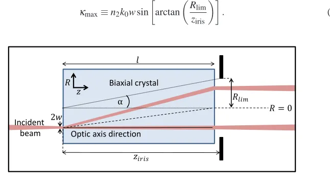
In practice the range over which Eqs. (5) and (6) are integrated is not infinite, rather the exper-imental apparatus will introduce constraints on these values [15] with the maximum contribu-tionκmaxbeing the maximum transverse wavevector component reaching the imaging device. Consider an iris of radius Rlimcentred on the conically diffracted beam and placed a distance zirisfrom the entrance face of the crystal, as seen in Fig. 6. The maximum transverse wavevector componentκmaxpassing through this iris is then

κmax≡n2k0w sin

arctan Rlim

ziris

. (14)

2

Optic axis direction Biaxial crystal

Incident beam

= 0 α

Fig. 6. The maximum transmissible transverse wavevector componentκmaxis determined by the radius of the iris Rlimand its position ziris. This transverse wavevector is given by κmax=n2k0w sinαwhereα=arctan(Rlim/ziris).

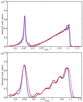
the observed intensity profile obtained by averaging several radial profiles and shows very good agreement. The rapid oscillations of the profile for 0.9≤ρ/ρ0≤1.1 are somewhat smoothed out in the experimental profile due to the effect of this averaging.

A variable iris was then inserted between the crystal and the biconvex lens, a distance of

ziris=40 mm from the entrance face of the crystal. When the iris was at its minimum setting, the limiting radius was Rlim=0.75 mm which is smaller than the radius of the crystal, and so using Eq. (14) we findκmax=19. Equation (8) was subsequently used to calculate the theoretical intensity profile shown in Fig. 7(b), compared with the experimentally observed profile, again showing very good agreement. The inner ring is less intense than the case with no iris as seen in Fig. 7(a), and it is also broader. The oscillations of the wedge-shaped feature have become more pronounced with longer periods than in Fig. 7(a).

0.8 0.85 0.9 0.95 1 1.05 1.1 1.15 0.0

0.2 0.4 0.6 0.8 1.0

0.8 0.85 0.9 0.95 1 1.05 1.1 1.15 0.0

0.2 0.4 0.6 0.8 1.0

ρ/ρ0

ρ/ρ0

Intensity (arb. units)

Intensity (arb. units)

(a)

(b)

4. Far-field propagation

The conically diffracted beam evolves as it propagates beyond the focal image plane. This evolution has been examined in the case of a Gaussian input profile [5, 16]. In this case the rings which form at the FIP spread out asζ increases and eventually the inner ring converges to produce a high intensity region in the centre of the beamρ =0 known as the ‘axial spike’. Whenρ01, the peak intensity of this axial spike occurs atζ ≈ρ02/3. A theoretical plot of the evolution over the range 0≤ζ ≤10 is shown in Fig. 8 generated using Eq. (8) with ρ0=7.2 and a(κ)given by Eq. (10).

11.5

1

0.5

0

-0.5

-1

-1.5 0 2 4 6 8 10ζ

ρ

/

ρ0

Fig. 8. Theoretical plot of the far-field evolution of a conically diffracted Gaussian beam generated using Eq. (8).

The propagation of a conically diffracted top-hat beam beyond the FIP was examined using the experimental arrangement in Fig. 9. A HeNe laser beam was directed onto a 100µm di-ameter pinhole and a biconvex lens of focal length f =10 cm was placed a distance u=20 cm after the pinhole. This produced an unmagnified image of the pinhole a distance v=20 cm after the lens. The profile of the laser beam at this point z=0 approximated a top-hat very well as shown by the red dots in Fig. 2(b). When a 22 mm long slab of KGd(WO4)2was inserted into the beam between the lens and z=0, the FIP occurred outside the crystal as determined by Eq. (4). A CCD with a pixel size of 6µm was mounted on a rail allowing movement in the ζ direction.

FIP CCD on rail Biconvex

lens HeNe laser

beam

Pinhole

v u

Biaxial crystal

z=0

Fig. 9. The experimental setup used to study how the conically diffracted top-hat beam evolves in space. The pinhole is imaged using a biconvex lens of focal length f to a point z=0 beyond the crystal, thus using Eq. (4) the FIP occurs outside the crystal at a distance v+l(1−1/n2)from the lens. z increases in the direction of beam propagation, and hence so do Z andζas given by Eq. (3).

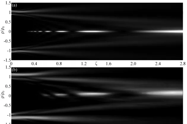
by Eq. (13). The theoretical profile is shown in Fig. 10(a). There is good agreement between theory and experiment and the presence of the predicted oscillatory axial spike is obvious; a feature which does not occur for the Gaussian input beam as seen in Fig. 8.

1.5

1

0.5

0

-0.5

-1

-1.5 1.5

1

0.5

0

-0.5

-1

-1.5 (a)

(b)

0 0.4 0.8 1.2 1.6 2.0 2.4 2.8

Fig. 10. Comparison of the theoretical evolution of the beam (a) with the observed evolution (b) in the case of a 50 µm radius top-hat beam. Image (b) was generated by stitching together a series of images taken at 1 mm increments in the direction of beam propagation.

The unusual structure of the evolution was examined more closely by generating a log plot of the intensity as shown in Fig. 11. It becomes apparent that the structure is very complex, with many rings of light which converge as the beam propagates. Indeed it appears that there are a multitude of intensity maxima where the rings converge along theρ=0 line for 0<ζ <0.4 which appear and disappear over extremely short distances.

1.5

1

0.5

0

-0.5

-1

-1.5_{0 0.2 0.4 1.6 1.8 6.0 6.2 6.4ζ}

ρ

/

ρ0

Fig. 11. A logarithmic plot of the far-field evolution of a conically diffracted top-hat beam, calculated using Eq. (8), in order to show the very complicated and intricate structure of the beam. It also demonstrates how the oscillating lobes along theρ=0 line are formed from many converging rings.

nature of the axial spike in a more rigorous way, we must use the following stationary phase approximation for the intensity of the conically diffracted beam atρ=0 taken from Jeffrey [15]:

I(ρ=0,ζ)≈πρ 2 0 2ζ3

a ρ0

ζ

2. (15)

Using the Fourier transform of the top-hat beam aT(κ)as given in Eq. (13) gives

I(ρ=0,ζ)≈πρ 2 0 2ζ3

_ρ0ζ J1 ρ0_ζ

2= π

2ζ

J1 ρ0_ζ

2. (16)

It will now be useful to use the following approximation for aνth_{order Bessel function of the} first kind, which is valid when x1:

J_ν(x)≈

2 πxcos

x−π₄−νπ₂, x1, (17)

→J1 ρ0_ζ

≈

2ζ

πρ0cos ρ0ζ − 3π

4

, ζ ρ0. (18)

⇒I(ρ=0,ζ)≈ π 2ζ

2ζ

πρ0cos2 ρ0ζ − 3π

4

=_ρ01 cos2 ρ0

ζ −

3π 4

. (19)

The form of the expression obtained in Eq. (19) brings us to an interesting conclusion—sinceζ does not appear in the factor before the oscillatory cos2term, the intensity of the maxima along ρ=0 is constant whenζ ρ0. Furthermore, we may now find the extrema of the function by taking the derivative and finding the values ofζ for which we get zero:

∂

∂ζI(ρ=0,ζ) = 2 ζ2cos

ρ0 ζ + π 4 sin ρ0 ζ + π 4

=0, (20)

⇒ζ±= ρ0

πn±1₄, n∈Z

+_{. (21)}

A simple calculation taking the derivative of Eq. (20) shows thatζ−corresponds to local max-ima, whileζ₊ corresponds to local minima. Examining Eq. (21) reveals that as n→∞with ζ→0, the separation between adjacentζ±values decreases at approximately the rate of 1/n2. This means the intensity along ρ=0 is an oscillatory function whose frequency increases rapidly as ζ →0. This feature suggests these beams may be used in super-resolution lens-ing [17], where high transverse wavevector components generate the intensity maxima in the region close toζ =0. Further work is anticipated in this potential application.

Whenζ is of the order ofρ0, the approximation in Eq. (18) breaks down and instead we must examine Eq. (16) to find that asζ→∞the intensity alongρ=0 trails off slowly to zero since

J1(ρ0/∞) =J1(0) =0.

5. Conclusion

the apparatus. The use of a variable iris to continuously vary the maximum transverse wavevec-tor component of the beam allowed very fine control of the features of the intensity profile, such as the width of the high-intensity inner ring, and the relative intensities of the inner ring and the wedge-shaped feature. The evolution of such a beam beyond the FIP was simulated using the theoretical model presented which yielded the unusual feature of an oscillating axial spike. This evolution was then observed experimentally and found to match extremely well with the prediction.

This unusual intensity profile may find applications in optical trapping since the strength of a trap depends on the gradient of the intensity [18]. Since in theory the intensity of the inner ring is limited by the apparatus being used, the use of high-quality components could lead to a very stiff trap indeed. It may also be used to create microstructures with very sharp features, or controlled using a variable iris as described in Section 3 to produce microstructures with tunable feature quality. We also anticipate further work using white light top-hat beams to generate novel polychromatic beam shapes, and to perform experiments in cascade conical diffraction [19] and the generation of Bessel beams [20] in order to compare the results with the case of conically diffracted Gaussian beams.

Acknowledgments