Soil Loss Mitigation using Synthetic Polymer under Simulated Condition

International Journal of Humanities and Social Sciences p-ISSN: 1694-2620 e-ISSN: 1694-2639 Vol. 8, No. 2, pp. 15-25, ©IJHSS

Soil Loss Mitigation using Synthetic Polymer under Simulated

Condition

Sheila G. Griengo,

Mindanao State University-Marawi City,

Romeo B. Gavino, Victorino T. Taylan, Sylvester A. Badua

Central Luzon State University,

Science City of Munoz, Nueva Ecija , Philippines

*Email address of corresponding author: [email protected]

Abstract

One of the effects of climate change is soil degradation which is mostly due to soil erosion. The use of anionic polyacrylamide (PAM) as a soil stabilizer is an emerging conservation practice for mitigating soil loss. PAM can be an alternative to traditional soil erosion control practices rather than mulching and slope profiling to control erosion. Generally the study aimed to assess the effect of using synthetic polymer (PAM) in mitigating soil loss under simulated condition. Specifically it attempted to install a locally fabricated rainfall simulator (spray-nozzle type) to evaluate the effectiveness of PAM at different rates (no PAM, 7.4 g of PAM per kg of soil and 14g of PAM per kg of soil) at different slope gradients (10, 35 and 60 degrees) and analyze the relationship of slope gradient versus sediment yield, and soil loss at different rainfall intensities. Different rates of PAM were applied in soil test boxes filled with medium loam of soil under simulated condition. Runoff volume was then collected every event to determine the sediment yield and soil loss. Data were analyzed using the Split-plot design with three replications and a regression analysis to determine their relationships. The results indicated that PAM applications significantly reduced sediment yield and soil loss at different rainfall intensities. The most effective rate of PAM applied in mitigating soil loss was found to be at a ratio of 14g of PAM per kg of soil. Sediment yield and soil loss were best fitted in a quadratic model in the form of a second degree polynomial equation. The relationships between slopes versus the above parameters being used were found to be non-linear. Moreover, the observed soil loss for every level of PAM was best modelled by the following coefficient of determination and their corresponding second degree polynomial equations for both rainfall intensities;

at 75 mm/h,

A₀ : SL = -0.0002s2 _{+ 0.0138s + 0.084; R² = 0.8845}

A40 : SL = -9E-05s2 + 0.007s + 0.0015 ; R² = 0.7964

A80 : SL = -6E-05s2 + 0.0044s - 0.021; R² = 0.8485, and ;

at 100 mm/h

A₀ : SL = -0.0008s2 _{+ 0.0652s - 0.06; R² = 0.9942}

A40 : SL = -0.0004s2 + 0.0251s + 0.0078; R²=0.9773

A80 : SL= -6E-05s2 + 0.0034s + 0.1223; R² = 0.7536.

Introduction

One of the most serious ecological problems here in the Philippines today is soil degradation. The most widespread process and most studied in the country is soil erosion (Asio, 2010). Soil is removed through erosion. When soil is removed it, results in the loss of soil fertility in the land where it came from. Erosion results to loss of organic matter and clay, topsoil and nutrients, and soil's capacity to retain nutrients and water. Moreover, lower infiltration rates and increased runoff are also a result of erosion due to the compaction and sealing of soil surface.

A vital resource for the production of renewable resources for the necessities of human life, such as food and fiber is soil thus, for better land use and conservation practices, identification and assessment of erosion problems plays an important role. Other than agronomic measure and other mechanical conservation of soils, another alternative practice is applying chemical amendments to modify the soil properties. Various polymers that stabilize soil surface structures and improve pore continuity have long been recognized as viable soil conditioners, (Orts et al., 2007. Many recent studies have shown that use of synthetic organic polymers, like polyacrylamide (PAM), as surface soil amendment results in benefits including reduction of runoff volumes, decrease in sediment yield, and stabilization of soil structure. The versatility of PAM is one of the aspects that make it attractive. The key to its effectiveness as a soil amendment is the way in which the polymer is adsorbs to the soil (Green et al., 2000).

Rainfall simulators have been used as tool in research in evaluating soil erosion and runoff from agricultural lands, high ways etc. It can be used either under laboratory conditions or in disturbed or natural soil and it is an important tool for the study of runoff generation and soil. The RS can expedite data collection because it has the ability to create controlled and reproducible artificial rainfall (Thomas and Swaify, 1989) and soils and management variables among locations can be easily compared (Sharpley et al., 1999). Thus, a rainfall simulator was designed and fabricated in this study to simulate rainfall and test the effect of synthetic polymer as soil stabilizer in mitigating soil loss in a simulated condition.

Generally, the study aimed to assess the effect of the synthetic polymer (PAM) on mitigating soil loss under simulated condition. Specifically it attempted to: (a) install a locally fabricated rainfall simulator (spray-nozzle type) to create a controlled condition for the study; (b) evaluate the effectiveness of the synthetic polymer (PAM) as soil stabilizer at different amount and at different slope gradients in mitigating soil loss; and (c) determine the relationship of slope versus sediment yield, and quantity of soil loss at different rainfall intensities.

Methods

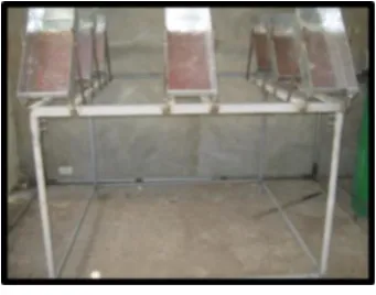
Rainfall Simulator Design

Figure 1. Rainfall Simulator

Wide Angle Full Cone Spray Tip (FL-10VC) centered over a 2.25-m2 _{plot to deliver}

simulated rain. . An electric pump was used to draw water from 200-liter reservoir to supply water to the nozzle thru a 20 mm G.I. pipe. Bypass line (made of three gates valves assembled together) just above the reservoir along with flow meter and pressure gauge before the nozzle assembly, were used to achieve the desired nozzle pressure. Just outside the pump outlet, plumbing system was equipped with gate valve and shutoff valve to turn the flow on and off without disturbing valves that control the pressure and flow rate. Sediment filter was used to reduce solid particulate transported by the water and remove suspended matter such as sand, silt, loose scale, clay, or organic material from the water that might clogged on the nozzle. Windscreen made from High Density Polyethylene plastic was used and attached to all sides of the frame, secured at the top to bottom so as not to affect rainfall simulation.

Calibration

Calibration was done using a method of 10 seconds discharge flow collected at the nozzle and measured whether or not it corresponds to the required volume of water for every simulation .The flow was adjusted until it met the desired discharge flow for every rainfall intensity.

Determination of Rainfall Uniformity Coefficient

To evaluate rainfall distribution in the soil test boxes, Christiansen Coefficient of Uniformity (CU) was used (Christiansen, 1942) as cited by Javellonar, 2013.

𝐶𝑈 = 100(1 − _𝑚𝑛 𝑥) (1)

where : CU = uniformity coefficient, %

m = mean value of simulated rainfall in the boxes, mm

x = absolute deviation of the individual observations from the mean,

n = number of observation

Soil Collection and Preparation

The soil test box with dimension of 40 cm x 20 cm x 10 cm was made from plain galvanized iron sheet formed into individual rectangular shapes riveted on all sides to keep it in shape, sealed on both sides to prevent water and soil leak from the boxes and with 5 cm lip on the forward end where runoff spills. Six 5 mm diameter drain holes were drilled on the boxes to allow water that infiltrated the soil to drain from the boxes and prevent ponding.

Nozzle Assembly

Sediment Filter, bypass line, Flow meter, pressure gauge

Samples of disturbed soil were used in the experiment for evaluation. Prior to packing of soil in the test boxes the approximate bulk density of the field was determined where soil samples were taken. Cheesecloth was placed on the bottom of the boxes to keep the soil from washing out of the holes in the boxes while allowing water to flow through when the soil was saturated. Boxes were then filled with soil half deep up to 3 cm and spread evenly.

The remaining 2 cm was added with soil mixed with dry PAM granules to achieve the appropriate weight based on the bulk density and until it was levelled with the lower lip of the boxes which was 5cm. After the desired weight was achieved by soil addition, tamping, and PAM application, the boxes were then subjected to pre-wetting treatment and left overnight.

Figure 2. Soil test boxes

Experimental Treatments

Each set-up was subjected into two different simulated storm intensities of 75 mm/h for 23 minutes and 100 mm/h for 12-minutes. Factors used in this study and their respective levels were the following:

A.) Main Plot: Slope Gradient S₁ = 10 degrees S2 = 35 degrees

S3 = 60 degrees

B.) Sub-Plot: Amount of PAM applied

A₀ = No PAM

A40 = 7.4 g of PAM per kg of soil

A80 = 14 g of PAM per kg of soil

Runoff Collection

The 5 cm forward edge lip of the boxes was attached with a Polyethylene (PE) plastic bag where runoff was allowed to flow during simulation. Runoff volume was then collected in each of the test boxes after a rainfall of predetermined duration, weighed and measured using a graduated cylinder.

Data Analysis

Data gathered was evaluated using the Split-Plot Design with three replications. Comparison

Regression analyses were likewise employed to determine the relationship of slope gradient versus sediment yield and soil loss at different rainfall intensities

Performance Indicators

In order to assess the effectiveness of the Polyacrylamide to prevent soil loss using the locally installed rainfall simulator, the following parameters were determined:

Sediment Yield (SY) - reflects the total amount of erosion over a specific area at a given

time. In this particular study, this was the mass of the oven-dried sediment collected over the area of the soil test box and duration of simulation. It was estimated using the formula adopted by Berboso, et al. (2008) as cited by Junio, et al. (2009).

𝑆𝑌 = 𝑠𝑚

𝐴𝑏𝑡 (2)

where: SY = sediment yield, g / m2 _-hr

Sm = mass of oven-dried sediment collected, g Ab = area of soil test box, m2

t = duration of simulation, h

Soil Loss (SL)– the total amount of soil erosion or loss generated from a given watershed

or a given area. The total soil loss from each storm event was calculated using Herweg and Ostrowski (1997);

SL = C (Sy/ A) (3)

where: C = 0.01 conversion factor ( g/m2 _{to tons/ha)}

SL = amount of soil loss for a storm event, tons/ha

Sy = amount of soil loss for the storm event, g A = area of soil test box, m2

Results and Discussion

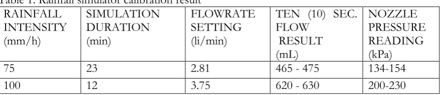
Calibration and Coefficient of Uniformity Test

Table 1 shows calibration result of the fabricated rainfall simulator. Effective area for the rainfall

simulator was 2.25 m2 _meters.

During the evaluation, the estimated mean Coefficients of Uniformity (CU) of the soil test boxes were 81.00% and 75.39% at rainfall intensities of 75 mm/h and 100 mm/h respectively. It depicts that 19% of the soil test boxes in 75mm/h and 24.61 % of the soil test boxes in 100 mm/h rainfall intensity did not have enough rainfall. The Coefficient of Uniformity tends to follow a normal distribution when the values is approximately 70% or higher (Esteves et al., 2000; Maroufpoor et al., 2010).

Table 1. Rainfall simulator calibration result RAINFALL

INTENSITY (mm/h)

SIMULATION DURATION (min)

FLOWRATE SETTING (li/min)

TEN (10) SEC. FLOW

RESULT (mL)

NOZZLE PRESSURE READING (kPa)

75 23 2.81 465 - 475 134-154

Soil Bulk Density and Textural Classification of the Soil Sample

The bulk density of the soil samples used in this study was 1.34 g/cm3_{. The test box was packed}

with soil based on the computed bulk density that determines the final weight of the soil in the box. With a soil height of 5cm at the box the approximate amount of soil was 5.4 kg/box. Textural classification shows that the sample has a soil type of medium loam with a composition of 49.94% sand, 30.11% silt, and 19.95% clay.

This soil type has an erodibility factor (K) of 0.42 at an organic matter of 2%. The K factor indicates susceptibility of certain soil to erosion. The higher the value depending on the type of soil, the more prone it is to erosion and vice versa.

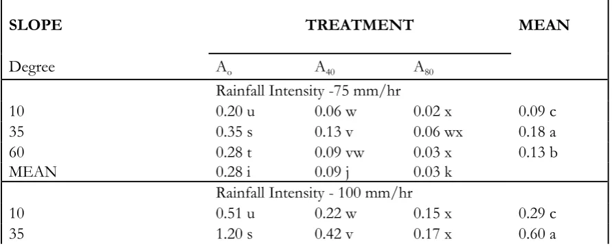
Soil Loss under Different Rainfall Intensity

Mean soil loss of PAM and slope gradient is shown in Table 2. It can be noted that treatment A80

recorded the lowest soil loss at rainfall intensity of 75 and 100 mm/h, followed by A₄₀ and A₀ or

no PAM. At 75 mm/h, soil loss increased as slope increased from 10 to 35 degrees but decreased as slope stretches up to 60 degrees. Similar trend of soil loss was also observed at rainfall intensity of 100 mm/h were soil loss was lowest at highest amount of PAM applied and at lowest slope gradient. Soil loss under 75 mm/h and 100 mm/h rainfall intensity were significantly affected by amount of PAM applied, slope gradient and interaction (PAM x Slope). Result of comparison among means for 100 mm/h intensity was noted in Table 2 where soil loss at slope 10 and slope 60 were significantly lower compared to slope 35 and significantly different

sediment yield was noted at A₀, A₄₀, A₈₀ amounts of PAM. On interaction of amount of PAM

and slope, the treatment combinations A80 at slope 10, A80 at slope 35, A80 at slope 60, A40 at

slope 60 had no significant differences on soil loss but they exhibited significant differences with

the other combinations. Highest soil loss of 1.20 ton/ha was observed at A0 slope 35 which is

significantly different from other treatment combinations. Significant reduction of soil loss could be attributed to PAM application on the soil test boxes. The result can be attributed to the migration of PAM granules in the pore spaces where they act as a mortar to limit erosion. Soil may become absorbed by activated PAM granules when PAM particles were wetted. They provide little benefit in terms of infiltration compared to the control (Peterson et.al, 2002).

The lower soil loss at 60 degree gradient was the result of a decrease in the horizontal surface area of the test box when it was inclined at a higher slope. When the horizontal surface area was decreased, less rainfall will be intercepted resulting to lower runoff and eventually lower soil loss (Javellonar, 2013).

Table 2. Mean soil loss (tons/ha) as affected by different amounts of PAM and varying degree of slope

SLOPE TREATMENT MEAN

Degree Ao A40 A80

Rainfall Intensity -75 mm/hr

10 0.20 u 0.06 w 0.02 x 0.09 c

35 0.35 s 0.13 v 0.06 wx 0.18 a

60 0.28 t 0.09 vw 0.03 x 0.13 b

MEAN 0.28 i 0.09 j 0.03 k

Rainfall Intensity - 100 mm/hr

10 0.51 u 0.22 w 0.15 x 0.29 c

60 0.85 t 0.15 xy 0.11 y 0.37 b

MEAN 0.85 i 0.26 j 0.14 k

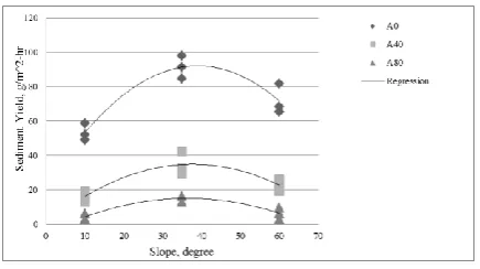
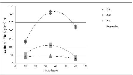
Slope Gradient versus Sediment Yield

Relationship between slope gradient and sediment is shown in Figures 3 and 4 for rainfall intensities 75 mm/h and 100 mm/h respectively. Regression analysis for both rainfall intensities indicates that sediment yield is best fitted in a quadratic model in form of second-degree polynomial equation.

Figure 3. Relationship of slope gradient vs sediment yield for 75 mm/h

The following are equations and coefficients of determination (R2_{) generated for every level of}

PAM applied at 75 mm/h,

A0 : SY = -0.0461s2 + 3.5957s + 21.913 ; R2 = 0.8845

A40 : SY = -0.0243s2 +1.8348s + 0.3913; R2 = 0.7964

A₈₀ : SY = -0.0157s2 _{+ 1.1391s - 5.4782; R}2 _{= 0.8485}

where 21.913, 0.3913 and 5.4782 are the intercept of the line on the Y-axis when slope is equal to zero, 3.5957 and -0.0461 ; 1.8348 and 0.0243; 1.1391 and -0.0157s2 are the first and second degree slopes of the line respectively, the amount of change in sediment yield for every unit of change in slope.

At 100 mm/h, the following are the equations and coefficients of determination (R2_),

A₀ : SY = -0.2174 s2 _{+ 17s - 15.652; R² = 0.9942}

A₄₀ : SY= -0.0991s2 _{+ 6.5478s + 2.0435; R² = 0.9773}

A80 : SY = -0.0157s2 + 0.8783s + 31.913; R² = 0.7536

where 15.652 is the intercept of the line on the Yaxis when slope is equal to zero, 17 and -0.2174 ; 6.5478 and – 0.0991; 0.8783 and -0.0157 are the first and second degree slopes of the line respectively, or the amount of change in sediment yield for every unit of change in slope;

where: SY = predicted sediment yield, g/m2_-h

Figure 4. Relationship of slope gradient versus sediment yield at 100 mm/h

A non-linear relationship was observed between slope gradient 10 to 60 degrees and sediment yield for all treatments under different rainfall intensities. That is, at lower slope gradient, sediment yield was likewise lower. When the slope gradient increased to 35 degrees, sediment yield also increases but when corresponding decrease in sediment yield was registered.

The observed decreased in sediment yield at a higher slope gradient of 60 degrees could be attributed to the smaller surface area of the soil test boxes. Furthermore the decrease in the horizontal surface area was the result of the shortened horizontal distance or length of the soil test boxes when it was tilted into a steeper slope (Javellonar, 2013).

On one of the study from Renner (1936), he found that the percentage of eroded area is different with the slope gradient after analysing the data of the Boise River watershed, Idaho in America. If the slope gradient exceeds a threshold value, the relationship takes inversely proportional form that is when the slope gradient exceeded 40°, the volume of soil erosion starts to decrease instead. In this particular study it was observed at 35 degrees slope gradient.

Slope Gradient versus Soil Loss

Figures 5 and 6 shows relationship between slope gradient and soil loss under different rainfall intensities. Regression analysis indicates that soil loss is best fitted in quadratic model at second degree polynomial equation. The following are equations and coefficients of determination ( R² ) generated for every level of PAM applied at 75 mm/h,

A₀ : SL = -0.0002s2 _{+ 0.0138s + 0.084; R² = 0.8845}

A40 : SL = -9E-05s2 + 0.007s + 0.0015 ; R² = 0.7964

A80 : SL = -6E-05s2 + 0.0044s - 0.021; R² = 0.8485

where 0.084, 0.0015, and -0.021 are the intercept of the line on Y-axis when slope is equal to zero, 0.0138 and -0.0002 ; 0.007 and -9E-05 ; 0.0044 and -6E-05 are the first and second degree slopes of the line respectively, or amount of change in soil loss for every unit of change in slope.

At 100 mm/h, the following are the equations and coefficients of determination (R2_),

A₀ : SL = -0.0008s2 _{+ 0.0652s - 0.06; R² = 0.9942}

A40 : SL = -0.0004s2 + 0.0251s + 0.0078; R²=0.9773

A80 : SL= -6E-05s2 + 0.0034s + 0.1223; R² = 0.7536

where - 0.06, 0.0078 , 0.1223 are the intercept of the line on Y-axis when slope is equal to zero, 0.0652 and -0.0008 ; 0.0251 and -0.0004 ; 0.0034 and -6E-05 are the first and second degree slopes of the line respectively, or amount of change in soil loss for every unit of change in slope;

where: SL = predicted soil loss, tons/ha S = slope gradient, degree

Non-linear relationship was also observed between slope gradient (10 - 60 degrees) and soil loss for all treatments under different rainfall intensities. At lower slopes, elevation is nearly flat; therefore velocity of the surface runoff is slow. When velocity is low, shear stress which may cause detachment of soil particles can also be slow. Therefore, when velocity of runoff is slow, little amount of sediment can only be transported downslope. At higher slope of 35 degrees, there is expected increase in surface runoff velocity so is with shear stress. Slope gradient also with velocity of runoff water could be at its maximum level capable of detaching and transporting significant amount of sediment hill (Javellonar, 2013).

Gradual decline was observed as the slope gradient further increased to 60 degrees. Observed decrease in soil erosion at higher slope gradient of 60 degrees could be attributed to smaller horizontal surface area of the soil test boxes when inclined to 60 degrees (Javellonar 2013). This result agrees with theory on “erosion as a function of slope” adapted from Pierce, FJ 1987, as cited by Javellonar, 2013. On the other hand, another factor which significantly reduced soil loss is application of PAM. Lentz et al. (1992) hypothesized that PAM could be used to decrease erosion since it can increase cohesiveness of soil at the surface which was tested in this study and reflected in the results showing its potential to mitigate soil loss on surfaces applied with PAM.

Figure 6. Relationship of slope gradient versus soil loss at 100 mm/h

Conclusions

1. The locally fabricated rainfall simulator (nozzle type) was effective in delivering the required rainfall intensity in this particular study.

2. At any given level of slope gradient under different rainfall intensities, Polyacrylamide (PAM) effectively acted as soil stabilizer that mitigates soil loss.

3. Treatment A80 at different slope gradients and rainfall intensities had significantly reduced

sediment yield and soil loss.

bx + cx2_{, where y represents the predicted value of sediment yield and soil loss while x is the}

slope in expressed in degrees. Moreover the generalized equations for soil loss obtained from the different amount of PAM were:

SL = -0.0002s2 _{+ 0.0138s + 0.084,}

SL = -9E-05s2 _{+ 0.007s + 0.0015,}

SL = -6E-05s2 _{+ 0.0044s - 0.021, and}

SL = -0.0008s2 _{+ 0.0652s - 0.06,}

SL = -0.0004s2 _{+ 0.0251s + 0.0078,}

SL= -6E-05s2 _{+ 0.0034s + 0.1223, for 75mm/h and 100 mm/h rainfall intensity}

respectively.

5. Using PAM as an alternative conservation has repeatedly been proven to be an effective tool where it is available. However the cost associated with amount of PAM application to a whole field or repeatedly applications may not be very the most practical way to control rain-induced erosion.

References

ASIO, V.B., 2010. Soil and Environment;soil and its relation to environment, agriculture, global warming, and human health. Retrieved on October 16, 2014 http://soil-environment.blogspot.com/search?q=soil+erosion

BERBOSO, J.L., G.P., PANIEL, A.C.C., PERLADA, and R.J.V., SAN DIEGO. 2008. Assessment of Combined Hydroseeding and Coconet Reinforcement to Control Soil Erosion. Unpublished Undergraduate Thesis, School of Civil Engineering and Environmental and Sanitary Engineering, Mapua Institute of Technology, Manila, Philippines.

ESTEVES M, PLANCHON O, LAPETITE JM, SILVERAI N, CADET P .2000. The Emire large rainfall simulator: design and field testing. Earth. Surf. Proc. Land. 25: 681-690.

GREEN, V.S., D.E., STOTT, L.D., NORTON and J.G., GRAVEEL. 2000. PAM Molecular Weight and Charge Effects on Infiltration under Simulated Rainfall. Soil Sci. Soc. Am. J., 64:1786–1791.

JAVELLONAR, R. P. 2013. Rice Straw Geoxtextile As Ground Cover For Soil Erosion Mitigation. Journal of Energy Technologies and Policy, 3(11).

KIBET, L.C., L.S., SAPORITO, A.L., ALLEN, E.B., MAY, P.J., KLEINMAN and F.M., HASHEM. 2014. A Protocol for Conducting Rainfall Simulation to StudySoil Runoff.

Lentz, R. D., I. Shainberg, R. E. Sojka, and D. L. Carter. 1992. "Preventing Irrigation Furrow Erosion With Small Applications of Polymers." Soil Sc!. Soc. Am. J. 56: 1926-1932.

MAROUFPOOR E, FARYABI A, GHAMARNIA H, MOSHREFI G 2010. Evaluation of uniformity coefficients for Sprinkler irrigation systems under different field conditions in Kurdistan Province (Northwest of Iran). Soil Water Res., 5: 139-145

ORTS, W. J., GLENN, G. M., IMAM, S. H., SOJKA, R. E. 2008. Polymer applications to control soil runoff during irrigation. PAM & PAM Alternatives workshop, Albany, California, US, 34 – 37. PETERSON, J.R., D.C, FLANAGAN, and J.K., TISHMACK. 2002. Polyacrylamide and Gypsiferous

Material Effects on Runoff and Erosion under Simulated Rainfall. American Society of Agricultural Engineers. Vol. 45.

SHARPLEY, A. N., T. C. DANIEL, R. J. WRIGHT, P. J. KLEINMAN, T. SOBECKI, R. PARRY, AND B. JOERN. 1999. National phosphorus project to identify sources of agricultural phosphorus losses. Better Crops 83(4): 12–14.

RENNER F G. 1936. Conditions influencing erosion of the boise river watershed.. V S Dept Agric Tech Bull, 528.

The Author