2008
Analyzing impacts on backorders and ending
inventory in MRP due to changes in lead-time,
demand variability and safety stock levels
James Duane Abbey
Iowa State University
Follow this and additional works at:
https://lib.dr.iastate.edu/rtd
Part of the
Business Administration, Management, and Operations Commons
, and the
Operational Research Commons
This Thesis is brought to you for free and open access by the Iowa State University Capstones, Theses and Dissertations at Iowa State University Digital Repository. It has been accepted for inclusion in Retrospective Theses and Dissertations by an authorized administrator of Iowa State University Digital Repository. For more information, please [email protected].
Recommended Citation
Abbey, James Duane, "Analyzing impacts on backorders and ending inventory in MRP due to changes in lead-time, demand variability and safety stock levels" (2008).Retrospective Theses and Dissertations. 15360.
Analyzing impacts on backorders and ending inventory in MRP due to
changes in lead-time, demand variability and safety stock levels
by
James Duane Abbey
A thesis submitted to the graduate faculty
in partial fulfillment of the requirements for the degree of
MASTER OF SCIENCE
Major: Business
Program of Study Committee:
Danny J. Johnson, Major Professor
Jennifer Blackhurst
Michael Crum
Charles Shrader
Iowa State University
Ames, Iowa
2008
1453896
2008Copyright 2008 by
Abbey, James Duane
Table of Contents
Abstract ... v
1 – Introduction ... 1
2 - Literature Review ... 3
2.1 - Total Cost of Ownership and Lead-Time ... 3
2.2 - Demand and Lead-Time Variability Studies ... 4
2.3 - Resilience, Flexibility and Lengthening Supply Chain Lead-Times ... 7
2.4 - Optimization Studies under Demand and Lead-Time Variability ... 8
2.5 - Ties to Strategic Sourcing ... 9
2.6 - Summary of Articles ... 10
2.7 - Summary of Literature Search Findings ... 11
3 - The Simulation Model ... 13
3.1 – Bill of Materials ... 13
3.2 - Capacity and Daily Regeneration ... 14
3.3 – Backorders ... 14
3.4 - Demand Distribution ... 15
3.5 - Forecast Methodology ... 16
3.6 - Lead-Time Distribution ... 17
3.7 - Steady State ... 20
3.8 - Safety Stock ... 21
3.9 - Batch Size ... 21
3.10 - Final Experimental Models ... 21
4 – Simulation Results and Findings ... 23
4.1 – Graphical Analysis ... 23
4.2 – Discussion of Results ... 26
5 - Analysis of Backorders ... 28
5.1 - Lead-Time Impact on End Products and Components ... 28
5.2 - Demand Variance Impact on End Products Across Safety Stock Levels ... 28
5.4 - Safety Stock Impact on End Products Across Demand Variability Levels ... 32
5.5 - Safety Stock Impact on Components ... 33
5.6 – Backorder Analysis for Components Combined Analysis ... 35
5.7 – Conclusions about Backorders ... 39
6 - Analysis of Ending Inventories ... 41
6.1 - Lead-Time Impact on End Products and Components ... 41
6.2 - Demand Variance Impact on Components Across Safety Stock Levels ... 41
6.3 - Safety Stock Impact on Components Across Demand Variability Levels ... 43
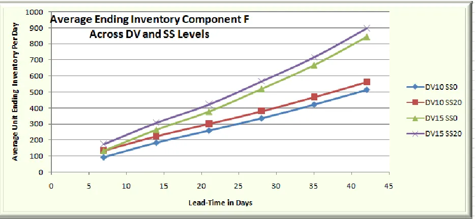
6.4 – Ending Inventory Analysis for Components ... 45
6.5 – Conclusions about Ending Inventories ... 47
7 - Formal Statistical Analysis of Lead-Time, Demand Variability and Safety Stock Main Effects ... 49
7.1 – Overall Model Analysis – Significant Effects and Interactions ... 49
7.1.1 – Backorder of End Product A ... 49
7.1.2 – Backorder of End Product B ... 50
7.1.3 – Backorder and Ending Inventory of Component C ... 51
7.1.4 – Backorder and Ending Inventory of Component D... 53
7.1.5 – Backorder and Ending Inventory of Component E ... 55
7.1.6 – Backorder and Ending Inventory of Component F ... 57
7.1.7 – Conclusions from Full Models ... 59
7.2 – Significant Effects Impact on End Products ... 59
7.2.1 – Backorder of End Product A ... 60
7.2.2 – Backorder of End Product B ... 62
7.3 – Significant Effects Impact on Components ... 63
7.3.1 – Backorder of Component C ... 63
7.3.2 – Ending Inventory of Component C ... 67
7.3.3 – Backorder of Component D ... 70
7.3.4 – Ending Inventory of Component D ... 73
7.3.5 – Backorder of Component E... 76
7.3.6 – Ending Inventory of Component E ... 78
7.3.7 – Backorder of Component F ... 81
7.3.8 – Ending Inventory of Component F ... 83
8 – Examining Zero Lead-Time Variability, Higher Levels of Safety Stock and Larger Batch Sizes ... 88
8.1 – Zero Lead-Time Variability ... 88
8.2 – Exploring Component Safety Stock at 40% of Gross Daily Requirements ... 92
8.3 – Component Batch Size at Two Weeks of Gross Daily Requirements ... 94
8.4 – The Exploratory Summary ... 96
9 – Conclusions ... 97
Works Cited ... 99
Abstract
Global sourcing represents one of the major focuses in many industries as a means to lower
costs. While global sourcing generally reduces per unit costs, the impact of global sourcing on total
costs throughout the supply chain often remains unrecognized. Increased lead-time due to global
sourcing represents one of the commonly unrecognized costs. Hence, the simulation model
developed in this study demonstrates the impact of lead-time length and variation as well as
variation in demand and safety stocks on the ending inventory and backorder levels in a two product
MRP system. The results show that backorders grow at a diminishing rate as a function of lead-time
while ending inventories show the opposite trend. In addition, the study shows that firms need to
more carefully consider the impact of lead-time. The study demonstrates that lead-time, not just
1 – Introduction
Global sourcing represents one of the major focuses in many industries as a means to lower
costs. According to total cost research discussed in Chapter 2, global sourcing generally reduces per
unit costs, but the impact of global sourcing on total costs throughout the supply chain often
remains unrecognized. In particular, costs such as purchase price and transportation are easily
calculated and recorded. However, costs due to quality issues, reverse logistics and particularly
increased lead-time often are unmonitored.
Costs associated with lead-time can be difficult to quantify. In general, as lead-time grows,
so does lead-time variability, which negatively impacts forecast accuracy. As forecast accuracy
worsens, end product and component backorders tend to increase. Moreover, low forecast
accuracy tends to lead to increased system buffers in the form of inventory. The buffers due to
increased lead-time come in the form of safety stock and increased batch size to achieve economies
of scale and transportation. While the larger safety stocks and batch sizes keep companies at
desired customer service levels, the inventory and related costs grow throughout the supply chain.
While some of the Total Cost of Ownership (TCO) literature discussed in Chapter 2
references the concept of lead-time costs, the actual quantification of the costs usually has been
ignored. Hence, this research examines the impact of lead-time, lead-time variability and forecast
accuracy on backorders and inventory levels throughout a two product MRP driven system.
Specifically, the extensive literature search found in Chapter 2 reveals a void in research that
quantifies lead-time and demand variability impacts and costs. In particular, very few research
papers either in TCO or operations quantify the impacts of lead-time and stochastic demand in MRP
systems. Hence, the model developed in this study demonstrates the impacts of lead-time length
and variation as well as variation in demand and safety stocks on the ending inventory and
backorder levels in a two product MRP system.
The study begins with a thorough search of literature (Chapter 2) on a range of studies from
qualitative TCO through highly mathematical iterative optimization processes that determine lot
sizing rules. In other words, the literature search includes a variety of papers that examine or
optimize safety stocks, lot sizes, lead-times, inventory levels and more. However, few of the studies
Chapter 3 presents the simulation model for the study. The simulation model discussion
outlines the various assumptions and random distributions necessary to make a working MRP
model. The structure of the MRP simulation provides a great variety of controllable parameters,
which permit in-depth investigation of impacts on ending inventories and backorders for both end
products and component parts/subassemblies. Chapter 3 provides details about the Bill of
Materials (BOM) for the product structure, insight into the random distributions of lead-time and
demand as well as details about the forecasting methodology and more.
Chapters 4, 5 and 6 present insights into the results of the simulation in intuitive terms. The
various graphics offer direct, visual meaning behind the results of changing lead-time, safety stock
and demand variability levels. In each Chapter, notes and conclusions give further details for the
reader to grasp the meaning of the results.
Chapter 7 presents a detailed statistical analysis of the simulation’s results. Chapter 7
breaks the statistical analysis into two parts. The first part examines the full model with all possible
interaction terms. The second part examines only those factors and treatments that offered
statistically significant changes to ending inventory and backorder levels.
Chapter 8 explores directions future research might lead as batch sizes, safety stock and
lead-time variability levels change more dramatically than in the main experiment detailed in
2 - Literature Review
This research began with a search of various Total Cost of Ownership (TCO) studies as well
as other related works on similar topics, such as demand variability, lead-time variability, optimal
lead-time policies and optimal inventory policies. The literature search revealed a void in research
that quantifies lead-time and demand variability impacts and costs. Hence, the simulation model
developed in this study demonstrates the impact of lead-time and lead-time variability as well as
demand variation on the overall inventory levels as well as backorders in an MRP system. As with all
studies, the assumptions of the research often dictate the general validity of the study to industry.
In this study, the goal of the MRP model is to remain both tractable and valid by allowing the
parameters to vary in ways that mimic real industry without excessive assumption sets. In
particular, this study integrates ending inventories and backorders in MRP under various lead-time
levels with differing levels of demand variability and safety stock. The results from the study reveal
that global sourcing and associated long lead-times lead to ever increasing levels of inventory and
backorders.
2.1 - Total Cost of Ownership and Lead-Time
Early TCO articles, mostly authored or co-authored by Ellram, discuss detailed conceptual
TCO frameworks with little quantitative analysis (Ellram L. 1993, Ellram L. M. 1994, Ellram & Siferd
1998). Ellram (1993) focuses on using TCO to analyze supplier development (pre-transaction),
purchase considerations (transaction) and supplier/material defect (post-transaction) impacts
(Ellram L. , 1993). While not a part of the current research, future research will integrate the
impacts of material defects. In their 1998 article, Ellram and Siferd discuss ways companies use TCO
as a link to strategic cost management (Ellram & Siferd, 1998). According to the article, 73% of
companies included in the case study used TCO to analyze purchases of components while 55% of
companies used TCO to make raw material purchases. The article also notes the link between TCO
and quality focus in 91% of the case study firms as well as use of best value (cost reduction overall)
items in 82% of firms. In other words, the components and raw materials in the BOM often
represent areas of focus in TCO. Unfortunately, the article does not discuss metrics to assess costs
of the components or raw materials.
Relatively recent TCO articles focus on offshore sourcing and the added costs of increased
not indicate how lead-times impact costs, merely that costs will go up as a function of lead-time
(Ferrin & Plank, 2002). Ferrin and Plank also include a large number of other cost drivers, such as
purchase price, shipping, transportation and quality costs with some indication of the impact of each
on the overall costs within a system. Mary Harding and Michael Harding attempt to make lead-time
cost rules of thumb, such as simple percent multipliers based on total lead-time (Harding M. L. 2001,
Harding M. 2007).
Most TCO articles note the common costs associated with manufacturing, such as purchase
price, transportation costs and related overhead. Some of the more recent articles such as Ferrin et
al. (2002) list many more cost drivers including quality, reverse logistics, lead-time, on-time delivery,
storage and more. While TCO literature extensively investigates potential costs, few of the papers
attempt to give metrics to quantify those costs. Thus, this research examines the impact of
lead-time and lead-lead-time variability in combination with demand variability and safety stocks on
backorders and inventory levels as a step toward understanding cost structures. As already noted,
this research is of particular use for firms considering long lead-time global sourcing strategies.
2.2 - Demand and Lead-Time Variability Studies
A number of studies examine the impact of lead-time and demand variability. One of the
earliest works in the field appeared in 1976. Whybark et al. attempt to investigate and categorize
uncertainty in MRP systems (Whybark & Williams, 1976). The authors assert that timing uncertainty
requires safety lead-time while quantity uncertainty requires safety stock. Future works affirm
much of the early work by Whybark and Williams. For example, Maloni et al. investigate the need
for special planning methods under stochastic times (Maloni & Benton, 1997). In effect,
lead-time variability comprises one of reasons manufacturers hold safety stock. Hence, much research
attempts to understand and quantify the relationship of lead-time variability with safety stock. A
later work by De Bodt et al. also confirms that safety stock represents an effective tool to manage
variation in production planning and scheduling as well as maintenance of customer service levels
(DeBodt & Wassenhove, 2001).
Other studies investigate the impact of external demand variability (end-product demand)
as a random variable. Grubbstrom et al. discover that proper buffering requires correctly
dimensioned safety stocks for the master production schedule (MPS) (Grubbstrom & Molinder,
Materials (BOM) under known lead-times (Enns, 1999). Enns finds that appropriate batch sizes can
lead to low work-in-process (WIP) inventory and low tardiness as well as consistent throughput
given a known lead-time. Enns’ later 2002 article demonstrates that performance effects due to
forecast bias and demand uncertainty impact the MPS and delivery performance quite differently
(Enns, 2002). Enns contends that increasing planned lead-time or safety stock will improve delivery
performance [metrics] depending on the nature of the tardiness. Enns further contends that
forecast bias offers no benefit over the use of safety stock. Talluri et al. discuss setting safety stock
levels using well established functions based on variable demand and variable lead-time at a case
study firm (Talluri, Cetin, & Gardner, 2004). Holsenback et al. employ the same well established
formulas in their 2007 article on safety stock as a function of variable lead-time and demand
(Holsenback & McGill, 2007).
Interestingly, demand variability is often assumed to follow a normal distribution. Benton
(1991) and Vollmann et al. (2005) are only a few examples (Vollmann, Berry, Whybark, & Jacobs
2005, Benton 1991). Eppen and Martin test the normality assumption by examining two safety
stock determination models with demand and lead-time as unknown, random parameters that must
be estimated (Eppen & Martin, 1988). The model uses exponential smoothing for demand
forecasts. From the exponential smoothing model, Eppen and Martin test for normality of the
errors and find that for long periods of lead-time (j=5 or 10), the normality of error assumption is
not always valid when demand across periods is correlated. When the demands are roughly
stationary, the normality assumption appears reasonable with five or more lead-time periods.
Moreover, Eppen and Martin’s experimental data shows that forecast error appears to grow as the
period’s lead-time increases. The research in this paper uses stationary demand with a modified
exponential smoothing forecasting method (see Section 3.5).
Also, several MRP specific articles investigate safety stocks as a function of lead-times and
batch/lot-sizes. One of the early and often cited works by Karmarkar notes that manufacturing
lead-times depend on lot sizes as well as utilization levels (Karmarkar, 1987). An earlier work by Gupta et
al. investigates the impacts of product structure, lot-sizes, position in the BOM as well as lead-time
uncertainty and lead-time bias (Gupta & Brennan, 1995). The authors find that costs tend to
increase as the lead-time uncertainty bias factors increase. The study also notes that uncertainty
applied at high levels of the BOM has the greatest cost impact. In their 1996 paper, Zijm and
& Buitenhek, 1996). In a comprehensive research paper, Koh et al. find that appropriate safety
stocks, lot-sizes and rescheduling provide the best means to cope with uncertainty (Koh, Saad, &
Jones, 2002). Koh et al. categorize and investigate a wide array of uncertainty sources and further
categorize the research that attempts to harness or understand the uncertainty. In a 2004 article,
Koh finds that unexpected lead-time increases (late delivery from suppliers) can have significant
impacts throughout the BOM, which is known to cause high inventory and system costs (Koh, 2004).
In addition, Koh finds that delays in a resource can ripple through the MRP system and delay all
batches held in queue, which increases inventory and system costs further—a finding verified in this
research. Jonsson and Mattsson discuss the need for analytically based safety stock levels in MRP
(Jonsson & Mattsson, 2008). The article’s survey data of PLAN companies (an affiliate of APICS) also
shows that among manufacturing companies, daily regeneration MRP and reorder point systems
remain the most popular inventory management systems for purchased inventory. Specifically, 61%
of manufacturers used MRP for parts inventory while 63% used MRP for semi-finished items
inventory. Curiously, 27% of the respondents even used MRP for distribution functions. Most
importantly, Jonsson and Mattsson find that lead-time accuracy and safety stock levels are the most
critical parameters for overall MRP performance. The research in this paper shows that extending
lead-times for materials only compounds the manufacturing lead-time increases as well as the
commensurate inventory increases.
Further studies try to quantify the penalties of shortened lead-times. Das et al. (discussed
below) find that suppliers attempt to charge a higher unit price for the small lot-size, short lead-time
orders (Das & Abdel-Malek, 2003). Chandra et al. argue similarly that while shortened lead-times
allow a reduction of safety stock, procurement costs may increase due to increased demands on
suppliers as well as increased transportation costs (expedited transportation) (Chandra & Grabis,
2008). The question of procurement costs will not be a part of the current research but may be a
consideration for future research.
Demand variability and lead-time articles offer an enormous depth of research potential as
seen in the myriad of articles cited above. The research in this paper picks up on the theme of
understanding and harnessing knowledge about demand variability, time and particularly
lead-time variability. None of the previous works have integrated the idea of long lead-lead-times in
conjunction with demand variability on the backorders and ending inventories within an MRP
2.3 - Resilience, Flexibility and Lengthening Supply Chain Lead-Times
Long supply chains lead to both greater complexity and increased variability (Christopher &
Peck, 2004). Christopher and Peck also assert that in-bound lead-times represent a major key for
supply chain velocity as well as supplier selection. Moreover, added complexity and variability
become particularly large problems when companies make decisions in isolation due to forecast
rather than demand driven systems. The Christopher and Peck article also discusses the need to
build a resilient supply chain that can help mitigate such risks.
Resilience can come in many forms. One often noted form is redundant or reserve
suppliers, some of whom are close to the final manufacturing site or point of sale (Chopra & Sodhi,
2004). Chopra and Sodhi specifically cite Cisco Systems’ use of slow, overseas suppliers for items
that are fast-moving, standardized and low risk. For slower-moving, non-standardized, high risk
items, Cisco uses more expensive local suppliers to achieve greater flexibility. In partial contrast,
Berger and Zeng argue that better communication and stronger ties can lead to lower risk as well as
more stability in the supply chain, even in the case of single sourcing or limited supplier sourcing
(Berger & Zeng, 2006). Their paper goes on to model the impacts of supplier disruptions, the
operating costs of multiple suppliers and the commensurate financial loss caused by all suppliers’
being down. Unfortunately, the research does not identify the potential downsides of increasing
lead-times even when those long lead-times are known. While integration of supply chain risk and
associated probabilities of the risks are beyond the current research, future research may benefit
from modeling some risk factors.
Supply chain flexibility and agility appear to tie in well with lead-time evaluation. Sharifi et
al. propose that increased speed (reduced lead-time) directly improves agility (Sharifi & Zhang,
1999). Other early papers on supply chain flexibility with regard to procurement often focus on the
importance of relationships between buyers and suppliers (Narasimhan, Jayram, & Carter, 2001).
Another early work by Svensson argues both qualitatively and quantitatively that outsourcing
appears to increase inbound material flow disruptions and related risks, both of which hurt agility
(Svensson, 2001). Later papers, such as Das et al., discuss the concept of flexibility in fixed order
quantities (lot-size) and lead-time tend to cause the most supply chain conflict due to a buyer’s ever
decreasing lead-time and smaller lot-size orders to accommodate demand variability. Moreover,
the article models and defines flexibility as the ability of firms in the supply chain to mitigate
procurement price increases and penalties under adverse conditions. Manzini et al. discuss the
benefits of added flexibility in the supply chain to handle capability variation (product mix) and
capacity variation (demand levels) in multi-cellular manufacturing systems (Manzini, Persona, &
Regattieri, 2006).
Verma studies the impacts on supply chain agility in a base stock model with stochastic
demand and fixed replenishment lead-time (Verma, 2006). Finally, in what may become a seminal
piece in defining supply chain flexibility and agility, Swafford et al. tie the concept of flexibility and
agility into multiple dimensions including procurement, manufacturing, distribution and overall
supply chain adaptability (Swafford, Ghosh, & Murthy, 2006). Swafford et al. further assert that
more stable lead-times could allow greater customer responsiveness.
The current study shows that increasing lead-times lead to significant increases in
backorders and ending inventory, two areas that flexibility and agility try to minimize. Moreover,
the findings show that increased lead-time can negatively impact a company’s ability to meet
customer needs. If a company also faces the potential of significant disruptions beyond the simple
demand and lead-time variability investigated in this study, the results could be quite negative for
overall supply chain resilience.
2.4 - Optimization Studies under Demand and Lead-Time Variability
Several previous research papers focus on optimizing lead-time and safety stock. Each
optimization model makes varying degrees of limiting assumptions. In a paper similar to this study,
Molinder investigates optimal lot-sizes, safety stocks and lead-times (Molinder, 1997). More
specifically, Molinder employs design of experiments to define various treatment levels based on
stochastic demand and lead-time to evaluate the impact on optimal lot-sizes, safety stocks and
safety lead-times. The study uses twelve treatment levels to investigate the impact of stochastic
demand and lead-times. The stochastic impact is dramatically lessened by choosing predetermined
factor/treatment combinations. Molinder also attempts to balance stockout costs with inventory
transforms with Gamma distributions to make safety stock decisions (Grubbstrom & Tang, 1999).
Their research shows that optimal safety stock levels tend to drop with reduced variance levels.
An early article by Yano attempts to optimize lead-time directly in a limited structure
two-level subassembly system (Yano, 1987). Chu et al. also investigate and propose an iterative
algorithm to minimize holding costs and backlogging costs under lead-time variability (Chu, Proth, &
Xie, 1993). Other researchers investigate use of Markov models in limited contexts to achieve
optimal lead-times to minimize backlogging and holding costs (Dolgui & Olud-Louly, 2002). Dolgui et
al. note that the assumption set required for modeling makes validity of the Markov model for
industry somewhat questionable. A much later work by Persona investigates super BOMs, modular
product design and safety stock as means to control the forecasts and forecast errors (Persona,
2007). Persona demonstrates the efficacy of the model in both make-to-order (MTO) and
assemble-to-order (ATO) contexts. The article also formulates a total cost of safety stock and demonstrates
the potential safety stock as well as logistics cost reductions in two industrial case studies. While
each of these works focuses more heavily on optimization than the current research, the field of
research into understanding and controlling lead-time and lead-time variability remains quite active.
Unfortunately, as Dolgui et al. note, the assumption sets to make inference can be somewhat
restrictive. Hence, as already noted, the current research tries to maintain a minimal assumption
set for modeling purposes.
In a loosely related paper, Sounderpandian et al. investigate optimization of order quantities
under long lead-times and uncertainty in finished good demands (Sounderpandian, Prasad, &
Madan, 2008). The optimization technique involves linear programming along with genetic
algorithms and stochastic optimization to determine optimal order quantities. The paper
demonstrates the model efficacy with an example application in the plywood industry.
Sounderpandian et al. stress the impact of long lead-times within the supplier’s intra-country supply
chain as well as the lead-times to move the product down the chain. Moreover, the authors note
that risk of loss and commensurate supply uncertainties are also higher in the developing nations.
2.5 - Ties to Strategic Sourcing
In an early work, Ellram and Carr argue that for true strategic sourcing, purchasers must
take an active rather than passive role in controlling material flows (Ellram & Carr, 1994). In effect,
level, strategic decision points. Other related articles discuss sourcing decisions for vertical
integration versus outsourcing of production under differing forms of uncertainty (Kouvelis &
Milner, 2002). Talluri and Narasimhan note that firms that engage in strategic sourcing must focus
on supplier capabilities such as management practices, process capabilities and more as opposed to
simple metrics such as cost (Talluri & Narasimhan, 2004). In other words, though taking inventory
costs as a function of lead-time and demand variability can be very useful for defining and
understanding costs, strategic issues beyond costs must also be considered.
2.6 - Summary of Articles
A chronological summary of the articles cited above appears in table 2.6.1.
Table 2.6.1: Summary of Cited Articles Lead-time and Demand Variability
Chandra and Grabis, 2008 Jons son and Mattsson, 2008 Holsenback and McGill, 2007 Koh, 2004
Talluri, Cetin and Gardner, 2004 Enns, 2002
Koh, Saad and Jones, 2002 DeBodt and Wassenhove, 2001 Enns, 1999
Maloni and Benton, 1997 Grubbstrom and Molinder, 1996 Zijm and Buitenhek, 1996 Gupta and Brennan, 1995 Benton, 1991
Eppen and Martin, 1988 Karmarkar, 1987
Whybark and Williams, 1976
Topic
Supplier penalties for short lead-times Criticality of analytically based safety stocks Applications of established safety stock formulas Ripple effect of material delays through the BOM Applications of established safety stock formulas Forecast bias and demand uncertainty impact MPS Best buffers to handle uncertainty
Safety stock to manage planning, scheduling & service Batch size impact on utilization through the BOM Planning needs to accommodate variability Proper safety stock buffering in the MPS
Integration of lead-time and capacity management MRP cost impacts due to variability and BOM position Safety stock levels with normally distributed demand Safety stock levels & normality of forecast error Lot size impacts on lead-time
Early work in MRP uncertainty buffers
Optimization Studies Related to Lead-time and Demand Variability
Sounderpandian, Prasad, & Madan, 2008 Persona, 2007
Dolgui and Olud-Louly, 2002 Grubbstrom and Tang, 1999 Molinder, 1997
Topic
Optimal order quantity in developing nations
Chu, Proth and Xie, 1993 Yano, 1987
Optimization of costs under lead-time variability Optimal lead-times in two-level subassemblies
Resilience, Flexibility and Lengthening Supply Chain Lead-Times
Berger and Zeng, 2006
Manzini, Persona and Regattieri, 2006 Swafford, Ghosh and Murthy, 2006 Verma, 2006
Christopher and Peck, 2004 Chopra and Sodhi, 2004 Das and Abdel-Malek, 2003
Narasimhan, Jayram and Carter, 2001 Svensson, 2001
Sharifi and Zhang, 1999
Topic
Optimizing number of suppliers
SC flexibility to handle capacity and capability variance Defining flexibility and agility in the supply chain Supply chain agility in the face of variability Resilience and dangers of longer supply chains Supply chain risks and industry reactions
Flexibility in lot-size & lead-time buyer/supplier conflict Flexibility of supplier relations
Outsourcing disruptions for inbound material flows Relation of lead-time to supply chain agility
Strategic Sourcing Links
Talluri and Narasimhan, 2004 Kouvelis and Milner, 2002 Ellram and Carr, 1994
Topic
Monitor and understand supplier capabilities Modeling impacts of outsourcing versus integration Lit review of strategic sourcing methods/research
TCO and TCO with Lead-Time
Harding M. , 2007 Ferrin and Plank, 2002 Harding M. L., 2001 Ellram and Siferd, 1998 Ellram L. M., 1994 Ellram L. , 1993
Topic
Discussion of practical lead-time cost metrics Exhaustive list of TCO cost factors
Simple cost metrics related to lead-time
TCO implementation in strategic cost management Standard vs. Unique TCO models
Framework for pre, post and transactions in TCO
Textbooks
Vollmann, Berry, Whybark, & Jacobs, 2005
Topic
Manufacturing Planning and Control Systems in SCM
2.7 - Summary of Literature Search Findings
The literature search reveals that demand variability and lead-time studies are plentiful and span
multiple topic areas. Supply chain agility, flexibility, resilience, planning, optimization as well as MRP
represent some of the many areas that note the various impacts due to lead-time on costs,
inventory levels, supply chain responsiveness and customer service. However, few of the papers
attempt to directly quantify the impact of excessively long lead-times due to global sourcing. TCO
papers sometimes note lead-time as a cost but only give minimal guidance on calculating the cost.
In resilience, flexibility and agility papers, increased lead-time throughout a supply chain emerges as
optimal safety stock levels, transportation methods and costs given set levels of lead-time. Yet, little
of the existing research attempts to model ever increasing lead-times due to global sourcing. In
3 - The Simulation Model
The model employs a two product structure with shared and unique components.
Moreover, the model uses symmetrical and asymmetrical components as well as unique
components to discern potential backorder and ending inventory differences. Further, distributional
assumptions came from various works cited in Chapter 2 of this work. For instance, many research
papers and supply chain texts generally assume that demand variability follows the normal
distribution (Vollmann, Berry, Whybark, & Jacobs 2005, Benton 1991). The following sections
discuss the experimental factors, batch sizes, steady state levels, forecasting methods, bill of
materials, MRP regeneration and other facets of the simulation model.
3.1 – Bill of Materials
The bill of materials (BOM) contains two end products (parents) and four component inputs.
Component C is a common component with symmetric requirements of 4 pieces per unit of end
product. Component D is unique to end product A with a requirement of one unit per unit of end
product A. Component F is unique to end product B with a requirement of four units per unit of end
product B. Component E is another common component with asymmetric requirements. End
product A requires one unit of component E while end product B requires four units of component
E. The different quantity and symmetry in components should provide both more validity and
information about potentially different ending inventory and backorder levels. Table 3.1.1 and
Figure 3.1.1 display the BOM in tabular and graphical form, respectively.
Table 3.1.1: Bill of Materials
Level 0 Level 1
Quantity Per
Parent
Product A
Component C 4
Component D 1
Component E 1
Product B
Component C 4
Component F 4
Figure 3.1.1: Bill of Materials Graphical Depiction
3.2 - Capacity and Daily Regeneration
The simulation models companies in an assemble-to-order (ATO) environment. Orders
arrive daily. Additionally, the MRP system regenerates daily. When orders for end products arrive,
the companies promise delivery 5 days out. In the simulation, production capacity is always
adequate to meet demand when component parts are available. The daily regeneration of the MRP
allows frequent determination of production requirements, demand levels and forecasts. Hence,
the error due to regeneration should be minimal when compared to a weekly or longer MRP
regeneration cycle. However, the planned order receipts created in a day freeze into the future for
the length of the lead-time (no change orders are allowed within the lead-time period). In other
words, the planned order receipts within the lead-time will always be zero – the manufacturer
cannot alter orders within the lead-time. In practical terms, once a shipment leaves a supplier, a
supplier cannot insert more components into the shipment. Since MRP is a forecast driven system,
the freeze period length can have a great impact on the overall performance of the MRP system.
Any demand changes within the lead-time that increase requirements beyond the predicted on
hand inventory generate additional backorders.
3.3 – Backorders
The simulation also runs under the assumption that no orders are lost. In other words,
A complete stockout of any one component required to make an end product generates a backorder
for the end product. To exemplify, if component E is entirely stocked out (on backorder), the
manufacturer can produce neither end product A nor B.
Further, when the supply of a component is not sufficient to meet the full demand for end
products, the shortage splits proportionally between products A and B. For example, assume end
product A has demand for 100 units while end product B also has demand for 100 units. However,
only 400 units of component E are available while all other component stocks are sufficient to meet
demand. The BOM shows that demand for 100 units of end product A leads to gross requirements
of 100 units of component E. Furthermore, the BOM shows that demand for 100 units of end
product B leads to gross requirements of 400 units of component E. Hence, component E has total
gross requirements of 500 units but only 400 units available. Since the requirements will be split
proportionally among products and 400/500 or 80% of the components required are available,
0.8*400 or 320 units of component E will be assigned to produce end product B while 0.8*100 or 80
units of component E will be assigned to produce end product A. In terms of finished goods, the
manufacturer will create 80 units of end product A and 80 units of end product B. In other words,
when X% of a component’s gross requirements are available, the manufacturer will produce X% of
the demand for end products A and B.
3.4 - Demand Distribution
The simulation models end product demand as normally distributed with a mean of 100 and
two standard deviation levels of 10 and 15. Mathematically,
) , (
~N
All random numbers were created in PROModel simulation package and rounded to the
nearest integer in Excel to create the required random vector of demand. Since the demand follows
a truly random distribution, no built-in cyclicality/seasonality exists.
3.5 - Forecast Methodology
The adaptive-response-rate single exponential smoothing (ADRES) appears to be a relatively
well behaved forecasting model for the randomly generated demand data (Wilson & Keating, 2002).
The ADRES adapts to the data to provide automatic adjustments for frequent changes in demand,
particularly when the model forecasts demand that is roughly symmetric around a mean value.
Forecasting a demand based on N(100, sigma), where sigma is 10 or 15, the ADRES represented an
easy choice. The ADRES in mathematical form:
t t t
t
t X F
F1
(1
) , s.t.,t t t
A
S
, where1 ) 1
(
t t
t e S
S
andA
t
e
t
(
1
)
A
t1t t t
X
F
e
Hence, alpha is a dynamic value based on the past period smoothed error (St) and absolute
smoothed error (At).
The ADRES model forecasts one period forward. Hence, since the data has no trend or
seasonality, the forecast for demand in day X is also the forecasted demand for every day through
the length of the lead-time. Thus, for a 42 day lead-time, the MRP system will generate
requirements based on a forecast schedule X+42 days into the future. Thus, if the forecast is
particularly far from the true demand for the period, the forecast error will carry through the entire
MRP freeze period.
The tracking signal provided a check of the biases of the forecasts. The tracking signal
divides the running sum of forecast errors (RSFE), a measure of bias, by the mean absolute deviation
(MAD), a measure of error, to give a picture of the true bias (in terms of MAD) in the system. To
constant at 0.2 with alpha varying as needed. A summary of the tracking signals for each forecasting
vector appears in Table 3.5.1.
Table 3.5.1: Tracking Signals on Forecast Error
Since the MRP followed a daily regeneration, forecasting also occurred daily and only one
day into the future. Random error showed up as quite large in some demand vectors and relatively
small in others—just as it would in real companies. For instance, A-4 and B-2 show particularly large
tracking signals in both the levels of demand variability. On the other hand, A-2 and B-1 show very
small tracking signals at both levels of demand variability. Hence, the simulation covers scenarios
from excellent forecasts down to poor, highly biased forecasts for greater general validity. While
discussion of various alternative forecasting methods is beyond the scope of this research, a real
company would be unlikely to achieve forecast accuracy significantly better than A-2 and B-1 or
worse than A-4 and B-2.
3.6 - Lead-Time Distribution
The simulation models the maximum early lead-time (MELT) as a gamma distribution. MELT
represents that maximum number of days early that a shipment can arrive for each potential
lead-time. As a conservative assumption, orders were only allowed to arrive early as a ratio of LT/7. In
other words, the maximum amount an order could arrive early was one day for a seven day
lead-time while a forty-two day lead-lead-time could have an order arrive up to six days early. In reality, the
variability of arriving early could be larger. As for arriving late, the gamma distribution has a right
skewed tail that allows orders to be significantly late but only rarely. All random digits were created
as vectors in PROModel and rounded to the nearest integer to create a vector of lead-times in Excel.
) , ( ~
)
(MELT Gamma
adTime
MaxEarlyLe or (
,
)s.t. 2 2 MELT MELT
whileMELT MELT
2Thus,
MELT
MELT
E
(
)
and
2 2 )
(MELT MELT
V
and
take on values to set the coefficient of variation equal to 0.3
2)
(
)
(
MELT
E
MELT
V
CV
=
1/2= 0.3Thus,
1/2 0.3 or
11
.
1111
Hence, the
takes on values such that the expected values are
) (MELT
E =
1 for 7 day LT,
11
.
1111
,
0.092 for 14 day LT,
11
.
1111
,
0.183 for 21 day LT,
11
.
1111
,
0.274 for 28 day LT,
11
.
1111
,
0.365 for 35 day LT,
11
.
1111
,
0.45and the standard deviations are
2 )
( )
(MELT V MELT
SD =
0.3 for 7 day LT
0.6 for 14 day LT
0.9 for 21 day LT
1.2 for 28 day LT
1.5 for 35 day LT
1.8 for 42 day LT
Table 3.6.1: Summary of Lead-Time Distribution Means and Variances
In effect, the mean of the Gamma distribution positions at the expected lead-time in days.
The Gamma distribution models the variance around the expected time. The higher the
lead-time, the wider the gamma distribution becomes as a function of the CV. Of course, the gamma
distribution truncates at zero but skews on infinitely at higher values. In other words, the expected
lead-time is the original lead-time in days while MELT represents the maximum number of days an
order can arrive early, which truncates at zero. The standard deviation of the MELT follows the right
skewed tail of the Gamma distribution. Hence, there is no direct truncation on the number of days
an order can be late.
LT Days Alpha Beta Beta^2 E(MELT) V(MELT) SD(MELT)
7 11.11111 0.09 0.0081 1 0.09 0.3
14 11.11111 0.18 0.0324 2 0.36 0.6
21 11.11111 0.27 0.0729 3 0.81 0.9
28 11.11111 0.36 0.1296 4 1.44 1.2
35 11.11111 0.45 0.2025 5 2.25 1.5
42 11.11111 0.54 0.2916 6 3.24 1.8
3.7 - Steady State
As noted in the forecasting section, the adaptive-response single exponential smoothing
forecasting system was set to hold beta constant at 0.2 with alpha varying as needed. Each
simulation replication generated 1000 days of data. To allow steady state to take effect, each
experimental run removed the first 150 observed days. Many simulation runs achieved steady state
much earlier than 150 days. Yet, consistency of the sample size and conservative estimates were
fortunate benefits from the data loss. Steady state was checked graphically for every treatment
level of the simulation. Law and Kelton’s text on simulation modeling describes the method
employed (Law & Kelton, 2000). Figures 3.7.1 and 3.7.2 show examples of output of twenty period
moving averages for various responses in the simulation.
Figure 3.7.1: Sample steady state graph for DV10, LT42, SS0 on Average Backorders of End Product B
3.8 - Safety Stock
Safety stock had no distributional assumptions. Instead, two main effect factor levels were
set with one additional pilot study level. The main effect levels were no safety stock and 20% of
daily demand. The pilot study level held safety stock at 40% of daily demand to observe the impact
of ever increasing safety stock levels on both backorders and ending inventory.
3.9 - Batch Size
The experiment held batch sizes fixed. While batch size was not part of the main
experiment, experimental subsets test the impact of batch size at extremes of lead-time (e.g., 7 and
42 days). Batch size for the main experiment was always lot-for-lot (L4L). As noted, orders could
occur in each period to meet forecast demand for the length of the lead-time.
3.10 - Final Experimental Models
The experiment’s main effects at the factor level:
Lead-Time (LT): Lead-time at factor levels 7, 14, 21, 28, 35 and 42 days [6 levels]
o Lead-time variance follows a Gamma distribution.
o As noted in the Lead-time distribution section, the coefficient of variation for
lead-time remained constant at 0.3.
Demand Variability (DV): Demand variability had factor levels 10 and 15 [2 levels]
o Demand was modeled using a normal distribution with mean 100.
Safety Stock (SS): Safety stock was set at either 0% or 20% of average daily gross
requirements for each component under the ratios described in the BOM. For example,
component C has gross average daily requirements of 800 units. Hence, safety stock at 20%
of average daily gross requirements leads to a safety stock of 160 units. [2 levels]
Treatment levels (combinations of the factor levels):
LT = 7, DV = 10, SS = 0
LT = 14, DV = 10, SS = 0
.
.
LT = 35, DV = 15, SS = 20%
LT = 42, DV = 15, SS = 20%
Hence, the main effects consisted of 24 treatment levels (LT*DV*SS = 6*2*2 = 24). Each
treatment level had n=5 replicates.
Other effects examined in subsequent experiments include zero lead-time variability, higher
safety stock levels and larger batch sizes. Each of these other effects contains between four and
twelve experimental runs.
Zero Lead-Time Variability: Additional experimental runs investigate the impact of zero
lead-time variability at each lead-time and demand variability level. [12 additional runs]
Safety Stock: Another set of additional runs investigates a 40% safety stock level at 7 and
42 days of lead-time with demand variability at sigma equal 10 and 15. [4 additional runs]
Batch Size: An additional set of experimental runs investigates the impact of increasing
batch size to two weeks (14 days) of average demand or simply 100*14 = 1,400 units
multiplied by the appropriate BOM multiplier for each component. [8 additional runs]
The total experiment contains 48 experimental runs with 240 replicates. 120 replicates were
used in the main experiment for the first 24 experimental runs. The remaining 24 experimental runs
split replicates across the additional questions of interest.
The responses of interest include end product backorders, component backorders and
component ending inventory. Each of these requires examination for statistical as well as practical
4 – Simulation Results and Findings
Chapter 4 focuses on the practical significance of the experimental results. All main effects
are statistically significant. Many interaction effects are not statistically significant. A full statistical
analysis appears in Chapter 7.
While the experiment/simulation tries to isolate the impacts of the main effects (lead-time,
safety stock and demand variability), the forecasting method (ADRES) and random error also cause
some of the effects seen. Most of the impact of the forecasting error should appear as random
error. Yet, while the simulation gives guidance on the general pattern due to main effects, other
impacts could make significant performance differences for real world manufacturers. The potential
exists that forecasting error added to the extremely poor results in terms of backorders and ending
inventory at the highest lead-times. Interestingly, the company with the very poor forecasting
(tracking signal average of 8.8 indicating bias) did not show up as consistently high or low in terms of
backorders or ending inventory. In other words, the MRP system appears to have smoothed the
biased forecast by adjusting requirements dynamically at each level of lead-time. In any case, as
with any simulation, validity is highest when the modeling assumptions (outlined in detail in Chapter
3) are met.
4.1 – Graphical Analysis
The responses of interest in the experiment include end product backorders, component
backorders and component ending inventories. As noted in the simulation model section, the main
effect experimental variables include safety stock, lead-time and demand variability. The trends
across lead-time in each of these responses can be seen most easily through graphical analysis. In
each case, the examined isolated effect is calculated as an average across all other effects.
The first set of graphs show that as lead-time grows, the level of end product backorders
grows. Likewise, as lead-time grows, the backorders and ending inventory of components also
grow. See Figures 4.1.1 – 4.1.3 to examine end product backorders, component backorders and
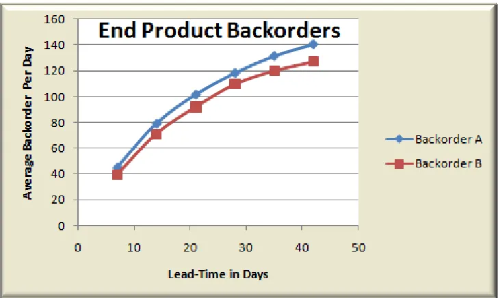
Figure 4.1.1: Average End Product Backorders across Lead-Time in Days
Figure 4.1.1 displays that end product backorders grow at a diminishing rate as lead-time
grows. Of course, other experimental factors generate different impacts on the growth of
backorders and ending inventory as discussed in Chapters 5 and 6. Another note is that backorders
of end product A appear to grow at a faster rate than the backorders of end product B, which
appears to be in part due to the more linear rate of increase in backorders for component D. At a
lead-time of 7 days, the difference between the two backorders averages only 5 units and grows to
13 units at a lead-time of 42 days. Since each end product has an average daily demand of
approximately 100, the difference could be significant for some firms.
As already noted, the average demand for each end product is approximately 100 units per
day. In other words, at 21 days of lead-time, the average backorders per day for end product A
exceed average daily demand. Likewise, end product B backorders exceed average daily demand at
approximately 24 days of lead-time. In other words, the systems are not serving customer needs
well at relatively short lead-times. Chapters 5 and 6 analyze the impact of safety stock and demand
Figure 4.1.2: Average Component Backorders across Lead-Time in Days
The BOM (section 3.1) shows that end item C has symmetric requirements of four units per
unit of end product A and four units per unit of end product B. Thus, the total gross requirements
for end product C are the highest of any component part in the experiment. As figure 4.1.2 displays,
backorders for component C represent the largest magnitude backorders of any component, as
expected. Both end products A and B require component E but asymmetrically. Figure 4.1.2 shows
the impact of the lessened requirements for component E. End product B requires four units of
component F per unit of end product B. End product A requires one unit of component D per unit of
end product A. Hence, the total backorders for D and F are the lowest among the backorders.
Each of the backorders shows a diminishing growth rate overall. However, the
symmetrically required component C average backorders grow faster than any other component
average backorder and do not appear to level off as quickly. Moreover, component D shows a
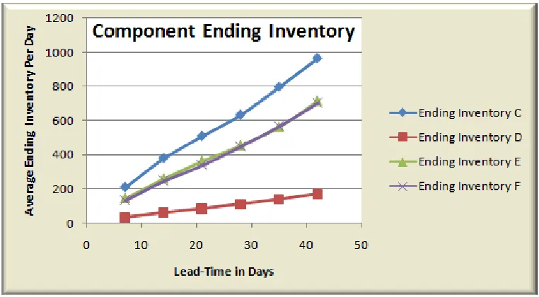
Figure 4.1.3: Average Component Ending Inventory across Lead-Time in Days
Unlike backorders, which show diminishing growth rates, ending inventory appears to
continue growth at an accelerating rate as lead-time grows. Due to the product structure (see
section 3.1), the ending inventory for component C grows the fastest while component D grows the
slowest, which helps explain the less dramatic growth rate in backorders for component D observed
in Figure 4.1.3.
Unexpected are the nearly identical ending inventories for components E and F.
Component F is an asymmetrically shared component while component E is unique to end product
B. Gross requirements are similar at 500 units per day of F and 400 units per day of E. However, the
nearly identical results, both in magnitude and trend, still represent somewhat of a surprise.
Quantitatively, ending inventory of component C grows from an average of approximately
200 units at a lead-time of seven days to nearly 1000 units at a lead-time of forty-two days. In
percentage terms, ending inventory for component C grows by nearly 500%. Other inventories
show similar percent gains at lower raw inventory levels.
4.2 – Discussion of Results
The overall results show that as lead-time grows, ending inventories and backorders of
component parts grow. As the backorders of component parts grow, so do the backorders of end
products. Backorders grow at diminishing rates while inventories grow at accelerating rates. Of
Two interesting notes emerge from the overall experimental picture. First, at only 21-24
days of lead-time, average end product backorders exceed average daily demand. In other words,
the system fails to keep backorder levels below demand at approximately a three week lead-time.
The result demonstrates that companies engaging in relatively long lead-time global sourcing should
exercise caution or at least recognize the potential for customer service issues. Second, average
ending inventories for a jointly, asymmetrically required component are nearly identical to the
average ending inventories of a lower gross requirement component required for only one end
product. In other words, the impact of asymmetry in component requirements does not appear to
have a major impact in the ending inventories. The gross requirements, rather than common parts
or symmetry of requirements, seem to have the largest impact on ending inventory levels.
Sections 5 and 6 discuss the impacts on ending inventory and backorders due to safety stock
and demand variability levels across lead-times. Each section breaks down the impacts of demand
5 - Analysis of Backorders
Chapter 4 notes that average end product backorders exceed average daily demand at only
21-24 days of lead-time. Chapter 5 analyzes some of the potential causes of the breakdown as well
as investigates other points of interest in the backorder patterns for both end products and
components.
5.1 - Lead-Time Impact on End Products and Components
In the overall system, backorders exceed average demand at 21-24 days of lead-time and
beyond. The following sections analyze the impacts of demand variance and safety stocks on
backorder levels at the various lead-times.
5.2 - Demand Variance Impact on End Products across Safety Stock Levels
Figures 5.2.1 and 5.2.2 show the average backorder level per day (averaged across safety
stock levels) for end products A and B, respectively. In each graph, two lines appear showing the
trend for demand variability at standard deviations 10 and 15. As discussed in section 3.4, end
product demand is modeled under a normal distribution with mean 100 and standard deviations of
10 and 15 units. In general, higher demand variability should lead to higher backorders. Figures
5.2.1 and 5.2.2 verify the intuition that greater demand variability leads to higher average levels of
backorders.
Figure 5.2.2: Average Backorder of End Product A at Demand Variability 10 and 15 across Lead-Time in Days
Both Figures 5.2.1 and 5.2.2 show very similar diminishing growth patterns for the average
backorder levels. The impact of increased demand variability on average backorder level is
somewhat consistent at each level of lead-time until a convergence at high lead-times. While the
end products do not show the convergence pattern as strongly as the components (discussed
below), the average backorder level starts to converge between the two demand variability levels at
the highest levels of lead-time. Hence, companies that are concerned about the demand variability
in their industry, something that is often regarded as outside an individual company’s control, can
see that increased lead-time worsens backorder levels but at a diminishing and somewhat
consistent amount for short and fairly long lead-times with a potential convergence at the longest
investigated lead-times.
5.3 - Demand Variance Impact on Components
Figures 5.3.1 through 5.3.4 show the average backorder level per day for components C, D, E
and F, respectively. In each graph, two lines appear showing the changes in trend due to end
product demand variability at standard deviations 10 and 15. End product demand variability
Figure 5.3.1: Average Backorder of Component C at Demand Variability 10 and 15 across Lead-Time in Days
Figure 5.3.1 shows a diminishing growth rate of average component C backorders with a
convergence at the highest level of lead-time (42 days). Examination of the standard deviations of
demand at 10 and 15 shows that demand variability 15 grows average backorders at a faster rate
than demand variability 10 until a sudden drop and convergence of the average backorder levels
after 35 days of lead-time.
Figure 5.3.2: Average Backorder of Component D at Demand Variability 10 and 15 across Lead-Time in Days
Figure 5.3.2 shows a diminishing growth rate of average component D backorders with
lead-time could be cause for modeling longer lead-times in the future to see if some sort of demand
variability cancelation occurs at very high lead-times.
Figure 5.3.3: Average Backorder of Component E at Demand Variability 10 and 15 across Lead-Time in Days
Figure 5.3.3 once again shows a diminishing growth rate of average component E
backorders. Component E shows little convergence at the highest lead-times.
Figure 5.3.4: Average Backorder of Component F at Demand Variability 10 and 15 across Lead-Time in Days
Figure 5.3.4 shows that component F follows a pattern similar to the other components with
a diminishing growth rate in average component backorders. Once again, component F shows
The convergence in three of the four components at 42 days of lead-time appears to be
worth future investigation. The result could be due to random error or some other factor. None the
less, future simulations likely should model longer lead-times to see if some sort of demand
variability cancelation occurs at very high lead-times.
5.4 - Safety Stock Impact on End Products across Demand Variability Levels
Figures 5.4.1 and 5.4.2 show the average backorder level per day across both levels of
demand variability for end products A and B, respectively. In each graph, two lines appear showing
the trend for safety stock levels of 0% and 20% of average gross daily requirements for components.
In other words, safety stock is not modeled for end products in the simulation since the
manufacturers produce and ship orders within the five day promised lead-time window (when
component stock is available). Figures 5.4.1 and 5.4.2 verify the commonly held notion that lower
component safety stock levels lead to higher average backorder levels for end products.
Figure 5.4.1: Average Backorder of End Product A at Component Safety Stocks 0% and 20% of Gross Daily Requirements
Figure 5.4.2: Average Backorder of End Product B at Component Safety Stocks 0% and 20% of Gross Daily Requirements
across Lead-Time in Days
Figures 5.4.1 and 5.4.2 show very similar diminishing growth patterns for the average
backorder levels across the two safety stock levels of 0% and 20% of gross daily component
requirements. The lines move in an almost perfectly parallel fashion, showing that the impact of
increased safety stock on average backorder level is roughly constant at each level of lead-time. In
fact, the difference between average backorders due to safety stock levels at each lead-time is
approximately constant at 14 units for end product A and 13 units for end product B. In effect,
safety stock simply reduces backorder levels by a roughly constant amount no matter the lead-time
level. Chapter 6 shows that the price for the diminishing backorder levels is actually a growing rate
of daily ending inventory.
5.5 - Safety Stock Impact on Components
Figures 5.5.1 through 5.5.4 graphically display the average backorder level per day for
components C, D, E and F, respectively. In each graph, two lines appear displaying the trend for
Figure 5.5.1: Average Backorder of Component C at Safety Stocks 0% and 20% of Gross Daily Requirements
across Lead-Time in Days
Figure 5.5.2: Average Backorder of Component D at Safety Stocks 0% and 20% of Gross Daily Requirements
Figure 5.5.3: Average Backorder of Component E at Safety Stocks 0% and 20% of Gross Daily Requirements
across Lead-Time in Days
Figure 5.5.4: Average Backorder of Component F at Safety Stocks 0% and 20% of Gross Daily Requirements
across Lead-Time in Days
Figures 5.5.1 through 5.5.4 all show roughly the same result—safety stock has a nearly
constant impact on the average backorder level across each level of lead-time. Unlike the average
backorder levels seen at different levels of demand variability, the average backorder levels at each
safety stock level do not converge or even change in pattern as a function of lead-time.
5.6 – Backorder Analysis for Components Combined Analysis
Figures 5.6.1 through 5.6.6 graphically display impacts on backorders due to changes in both
Figure 5.6.1: Average Backorder of End Product A at all Safety Stock and Demand Variability Levels across Lead-Time in
Days
Figure 5.6.1 shows that DV10-SS0 and DV15-SS20 appear to be approximately the same. All
trends are nearly the same.
Figure 5.6.2: Average Backorder of End Product B at all Safety Stock and Demand Variability Levels across Lead-Time in
Figure 5.6.2 once again shows that DV10-SS0 and DV15-SS20 appear to be approximately
the same at each mean level. As with end product A, all trends are nearly the same for every
treatment level.
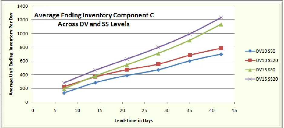
Figure 5.6.3: Average Backorder of Component C at all Safety Stock and Demand Variability Levels across Lead-Time in
Days
Figure 5.6.3, the graphic for component C, shows that DV10-SS0 and DV15-SS20 appear to
be similar at low lead-times but diverge at high lead-times. The trends in the treatment levels show
some variability, particularly at the longest lead-times.
Figure 5.6.4: Average Backorder of Component D at all Safety Stock and Demand Variability Levels across Lead-Time in
Figure 5.6.4 for component D shows somewhat less variability than Figure 5.6.3 (component
C). DV10-SS0 and DV15-SS20 appear similar at low lead-times but diverge at high lead-times.
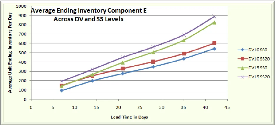
Figure 5.6.5: Average Backorder of Component E at all Safety Stock and Demand Variability Levels across Lead-Time in
Days
Figure 5.6.5 for component E shows somewhat less variability than Figure 5.6.3 (component
C) but more variability than 5.6.4 (component D). The added variability likely stems from the joint
requirements by both end products for components C and E. Yet again, DV10-SS0 and DV15-SS20
appear to be similar at low lead-times but diverge at high lead-times.
Figure 5.6.6: Average Backorder of Component F at all Safety Stock and Demand Variability Levels across Lead-Time in