Analysis of a Stochastic Predator-Prey Model in Polluted Environments

(1)

Analysis of a Stochastic Predator-Prey Model in

Polluted Environments

Huajuan Zhou, Meng Liu

∗

Abstract—In this paper, a stochastic predator-prey popula-tions model in polluted environments is proposed and investi-gated. We first study the existence, uniqueness and boundedness of the global positive solution. Then we establish the sufficient conditions for extinction, non-persistence in the mean and weak persistence in the mean of the predator and prey populations. The threshold between weak persistence in the mean and extinction for each species is obtained. Finally, we study the global asymptotic stability of the solution. Our results reveal that the more the number of random noises, the easier the species go to extinction.

Index Terms—environmental pollution, stochastic noises, per-sistence, extinction.

I. INTRODUCTION

E

NVIRONMENTAL pollution by modern industry, a-griculture, and other human activities is one of the most important socio-ecological problems in the world today. The presence of toxicant in the environment is a great threat to the survival of the exposed living beings. This motivates scholars to analyze the survival of populations in polluted environments and to establish the persistence-extinction thresholds of the populations.

In recent years, many scholars have studied the survival of populations with toxicants effect by establishing mathemat-ical models. Hallam and his colleagues did pioneering work in [1], [2], [3], where the authors studied some deterministic population systems with toxins effect and established the theoretical persistence-extinction thresholds for their models. From then on, many deterministic models in polluted envi-ronmrnts were proposed and analyzed. For example, Hallam and Ma [4], Ma et al. [5], [6], Freedman and Shukla [7], Wang and Ma [8], Buonomo et al. [9], Srinivasu [10] and He and Wang [11] proposed some single-species popula-tion models in polluted environments and established the persistence-and-extinction thresholds for their models. Liu and Ma [12] studied the persistence-and-extinction thresholds for two-species Lotka-Volterra models with toxins effect. Ma et al. [13] and Pan et al. [14] extended the threshold results in [12] to n-dimensional food chain model and n -dimensional factualistic system, respectively. Liu at al. [15],

Manuscript received 21 April, 2016; revised 12 May, 2016. This work was supported by the National Natural Science Foundation of China (Nos. 11301207), Project Funded by China Postdoctoral Science Foundation (2015M571349 and 2016T90236), Natural Science Foundation of Jiangsu Province (No. BK20130411), Natural Science Research Project of Ordinary Universities in Jiangsu Province (No. 13KJB110002), Qing Lan Project of Jiangsu Province (2014), Science and Technology Support Plan Project of Huaian (HAR2015013), Natural Science Foundation of Heilongjiang Province (No.A201420).

M. Liu is with the School of Mathematical Science, Huaiyin Normal University, Huaian 223300, PR China, and School of Mathematics and Statistics, Northeast Normal University, Changchun 130024, Peoples Re-public of China. E-mail: [email protected]

H. Zhou is with Huaiyin Normal University.

[16], Jiao et al. [17] and Li and Chen [18] considered the population models in polluted environments with pulse input of environmental toxins.

However, in the nature world the growth of population is inevitably affected by the random interference factors ([19], [20]). Thus it is important to study stochastic population models in polluted environments and to reveal the effects of random noises on the dynamics of populations. In this area, Gard did pioneering work in [21], where he first proposed a stochastic single-species model with toxins effect and investigated the dynamics of the model by supposing that the concentration of toxicant in the organism is a constant. Be-sides, Liu and Wang [22] obtained the persistence-extinction threshold for a stochastic logistic model in polluted envi-ronments. From then on, stochastic population models in in polluted environments have received great attention and have been studied extensively owing to their theoretical and practical significance (see e.g., [23]-[29]). Especially, taking into account the fact that predator-prey model is one of the most important models in biomathematics and ecology, Wang [24] has investigated the following stochastic predator-prey model in polluted environments:

                                  

dx1=x1[r10−r11C0(t)−a11x1−a12x2]dt +α1x1dB1(t),

dx2=x2[−r20−r21C0(t) +a21x1−a22x2]dt +α2x2dB2(t),

dC0(t)

dt =a1Ce(t) +d1θβ/a1−(l1+l2)C0(t),

dCe(t)

dt =−hCe(t) +u(t),

(1)

where x1(t) represents the size of the prey population at

timet; x2(t) stands for the size of the predator population

at timet;ri0>0is the growth rate of the speciesi;ri1≥0

denotes the speciesi’s dose-response parameters for toxicant concentration in the body;C0(t)represents the concentration

of toxicant in the organism at timet; aii >0 is the

intra-specific competition coefficients of speciesi;a12>0stands

for the capture rate;a21>0measures the efficiency of food

conversion; B1(t) and B2(t) are two independent standard

Brownian motions defined on a complete probability space

(Ω,F,P) with a filtration {Ft}t_∈R+ satisfying the usual

conditions (i.e., it is right continuous and increasing while

F0 contains all P-null sets); αi(i = 1,2) stands for the

intensity of the random noises; Ce(t) is the concentration

of toxicant in the environment at timet;a1Ce(t)represents

the organism’s net absorption amounts of toxicant from the environment; d1θβ/a1 is the organism’s net absorption

amounts of toxicant from the food;(l1+l2)C0(t)represents

IAENG International Journal of Applied Mathematics, 46:4, IJAM_46_4_06

(2)

the reduction of poison due to the metabolism and excretion; Parameters a1, d1(≤ a1), θ, β, l1 and l2 are positive

con-stants;a1represents the per unit mass organism’s absorption

rate of toxicant from the environment; d1 stands for the

per unit mass organism’s rate of toxicant from the food;

θ represents the concentration of toxicant in the resources;

β is the per unit mass organism’s intake rate of toxicant from the food;l1andl2are the decomposition and emission

rates of the toxicant in the organism, respectively; h > 0

is the environment’s ability to clean up poison; u(t) ≤U2

represents emission rate of environmental toxicant. Wang [24] has obtained the persistence-extinction threshold for model (1).

Based on the study [24], we find some interesting prob-lems:

(Q1) Model (1) assumes that the parametersr10andr20 are

affected by independent random noises. However, in the nature world, the random noises on r10 and r20

may or may not correlate to each other ([19]). For example, rain may affect bothx1 andx2. Thus what

happens if bothr10 andr20 are affected by correlated

random noises?

(Q2) Boundedness is an important properties for population models, which was not investigated in [24]. Then when the solution of the model is bounded?

(Q3) In the study of population models, the global asymp-totic stability of the solution is one of the most inter-esting topics. However, [24] did not consider global asymptotic stability of the solution.

The aims of this paper are to study the above problems. Sup-pose that ri0 affected by n independent standard Brownian

motions, then we obtain the following stochastic model:

                                      

dx1=x1[r10−r11C0(t)−a11x1−a12x2]dt

+x1

n ∑

i=1

α1idBi(t)

dx2=x2[−r20−r21C0(t) +a21x1−a22x2]dt

+x2

n ∑

i=1

α2idBi(t)

dC0(t)

dt =a1Ce(t) +d1θβ/a1−(l1+l2)C0(t)

dCe(t)

dt =−hCe(t) +u(t)

(2)

with initial data

xi(0)>0, C0(0) =Ce(0) = 0

where α1i, α2i are constants, Bi(t), (1 ≤ i ≤ n), are

in-dependent standard Brownian motions defined on(Ω,F,P). Clearly, if α11 ̸= 0, α1i = 0, 2 ≤ i ≤ n, α21 ̸= 0 and α2i= 0,2≤i≤n, then model (2) becomes model (1).

The rest of the paper is arranged as follows. In Section 2, we show that for any given initial data, model (2) has a unique global positive solution. Then in Section 3, we establish the sufficient conditions for stochastic boundedness of the solution. We carry out the survival analysis for model (2) in Section 4. Sufficient conditions for extinction, non-persistence in the mean and weak non-persistence in the mean of the species are established. The threshold between extinction

and weak persistence in the mean is obtained for each species. Afterwards, we investigate the global asymptotic stability of model (2) in Section 5. In the last section, we give some conclusions.

II. EXISTENCE AND UNIQUENESS OF THE SOLUTION C0(t)andCe(t)are the concentrations of toxicant, hence

we must give some conditions under which 0 ≤ C0(t) < 1, 0≤Ce(t)<1. In fact, the last two equations in model

(2) are linear with respect to C0(t) andCe(t), it is easy to

obtain their explicit solutions, so we have

Lemma 1. For model (2), if 0 < a1+d1θβ/a1 < l1 + l2, U2 ≤ h, then 0 ≤ C0(t) < 1,0 ≤ Ce(t) < 1 for all

t∈R+ a.s.

From now on, we always assume that0< a1+d1θβ/a1< l1+l2, U2≤h. We concentrate on the following subsystem

of model (2):

                  

dx1=x1[r10−r11C0(t)−a11x1−a12x2]dt

+x1

n ∑

i=1

α1idBi(t)

dx2=x2[−r20−r21C0(t) +a21x1−a22x2]dt

+x2

n ∑

i=1

α2idBi(t).

(3)

System (3) is a population model, so we should first give some conditions under which (2) has a global positive solution.

Theorem 1. For model (3), if aij >0, then for any given

positive initial value x(0) = (x1(0), x2(0)) ∈ R2+, there

exists a unique solution x(t) = (x1(t), x2(t)) to model (3)

a.s. (almost surely) and this solution does not leaveR2 + with

probability 1.a.s.

Proof: Since the coefficients of system (3) satisfy the local Lipschitz condition, so for any given initial conditions

x(0) = (x1(0), x2(0))∈R2+, there exists a unique local

sat-urated solution x(t) = (x1(t), x2(t))defined on t∈[0, τe],

whereτeis the time of the explosion ([30]). In order to prove

this is a general solution, we only need to prove τe = ∞.

Letn0>0 be sufficiently large such that all components of x(0)are on[1/n0, n0]. For every integern > n0, define the

stopping time

τn= inf{t∈[0, τe] :xi(t)≤

1

n or xi(t)≥n},

where we always set inf∅ = ∞. Obviously, τn increases

monotonically with respect ton. Letτ_∞= lim

t→+∞τn, hence τ_∞≤τe. Now we need to proveτ∞=∞. If it is false, we

can find a positive constantT >0 andε∈(0,1) such that

P {τ_∞<∞}> ε.

Then there exists an integern1≥n0 satisfying

P {τn< T}> ε , n > n1 (4)

Define a functionV(x)which is fromR2+toR+as follows:

V(x) =a21(x1−1−lnx1) +a12(x2−1−lnx2).

IAENG International Journal of Applied Mathematics, 46:4, IJAM_46_4_06

(3)

This function is non-negative because

u−1−lnu≥0, u >0.

According to Itˆo’s formula, we can see that

dV(x(t)) =a21(x1−1)

[

[r10−r11C0(t)−a11x1

−a12x2]dt+

n ∑

i=1

α1idBi(t) ]

+ 0.5a21

n ∑

i=1 α2₁_idt

+a12(x2−1)

[

[−r20−r21C0(t) +a21x1

−a22x2]dt+

n ∑

i=1

α2idBi(t) ]

+ 0.5a12

n ∑

i=1 α2₂_idt

=

[

0.5a21

n ∑

i=1

a21i+ 0.5a12

n ∑

i=1

α22i−r10a21+r20a12

+a21r11C0(t) +a12r21C0(t) + [r10a21+a11a21

−a12a21−a21r11C0(t)]x1+ [−r20a12+a12a21 +a12a22−a12r21C0(t)]x2−a11a21x21−a12a22x22

]

dt

+a21(x1−1)

n ∑

i=1

a1idBi(t) +a12(x2−1)

n ∑

i=1

a2idBi(t)

=G(x)dt+a21(x1−1)

n ∑

i=1

a1idBi(t)

+a12(x2−1)

n ∑

i=1

a2idBi(t),

(5) where

G(x) = 0.5a21

n ∑

i=1

a21i+ 0.5a12

n ∑

i=1

α22i−r10a21

+r20a12+ +a21r11C0(t) +a12r21C0(t) +[r10a21+a11a21−a12a21−a21r11C0(t)]x1 +[−r20a12+a12a21+a12a22

−a12r21C0(t)]x2−a11a21x21−a12a22x22.

Obviously, there is a positive constant G1 > 0 such that G(x)< G1. Substituting this inequality into (5) gives

dV(x(t)) ≤G1dt+a21(x1−1)

n ∑

i=1

a1idBi(t)

+a12(x2−1)

n ∑

i=1

a2idBi(t).

Therefore,

∫ τn∩T

0

dV(x(t))≤

∫ τn∩T

0

G1dt

+

∫ τn∩T

0

[

a21(x1−1)

n ∑

i=1

a1idBi(t)

+a12(x2−1)

n ∑

i=1

a2idBi(t) ]

.

Taking the expectation on the both sides, we have

E(x(τn ∩

T))≤V(x(0)) +G1E(τn ∩

T)

≤V(x(0)) +G1T.

(6)

LetΩn={τn≤T}, then by (16), we have P(Ωn)≥ε.

Note that for anyω∈Ωn, there is aisuch thatxi(τn, ω) =n

or xi(τn, ω) = 1/n. Therefore, V(x(τn, ω)) does not less

than

min

{

a21(n−1−lnn), a12(n−1−lnn),

a21

(

1

n−1 + lnn

)

, a12

(

1

n−1 + lnn

)}

.

That is to say,

V(x(0)) +G1T ≥E[1Ωn(ω)V(x(τn)))]

≥εmin

{

a21(n−1−lnn), a12(n−1−lnn),

a21

(

1

n−1 + lnn

)

, a12

(

1

n−1 + lnn

)}

,

where1Ωnis the index function ofΩn. Lettingn→ ∞gives

contradictory.

∞> V(x(0)) +G1T =∞.

This completes the proof.

III. BOUNDEDNESS OF THE SOLUTION

In the previous section, we have shown that model (3) has a unique global positive solution. Now let us show that the solution is stochastically bounded.

Definition 1. Model (3) is said to be stochastically bounded, if for∀ε >0, there is a positive constantK such that

lim inf

t→+∞P{xi(t)≤K} ≥1−ε, i= 1,2.

Theorem 2. Let (x1(t), x2(t)) be a solution to (3) with

initial value (x1(0), x2(0))∈R2+. Ifa22> a21, then model

(3) is stochastically bounded.

Proof: To begin with, let us show that for any p >1, there existsGi(p)such that

E[xp_i(t)]≤Gi(p), i= 1,2.

Define

V(x) =xp₁,

wherep >1. Applying Itˆo’s formula leads to

dV(x) =pxp₁

[

r10−r11C0(t)−a11x1−a12x2

+0.5(p−1)

n ∑

i=1 α2₁_i

]

dt+pxp₁

n ∑

i=1

α1idBi(t).

Making use of Itˆo’s formula again toet_V_(x)_{results in}

d[et_V_{(x)] =}_et_V_(x)dt₊_et_dV_(x)

=et_xp

1dt+etpx

p

1

[

r10−r11C0(t)−a11x1−a12x2

+0.5(p−1)

n ∑

i=1 α2₁_i

]

dt+petxp₁

n ∑

i=1

α1idBi(t).

Taking expectations on both sides, we can obtain that

E[et_xp

1] ≤x

p

1(0) +pE

∫ t

0

esxp₁(s)

[

1/p+r10

+0.5p

n ∑

i=1

α2₁_i−a11x1(s)

]

ds

≤xp₁(0) +

∫ t

0

esL1(p)ds =xp₁(0) +L1(p)(et−1),

IAENG International Journal of Applied Mathematics, 46:4, IJAM_46_4_06

(4)

where

L1(p) =

[

1 +pr10+ 0.5p2

n ∑

i=1 α2₁_i

]p+1

(p+ 1)p+1_ap 11

.

Thus there exists aT >0 such that

E[xp₁(t)]≤1.5L1(p)

for all t > T. At the same time, an application of the continuity of E[xp₁(t)] results in that there exist L˜1(p)>0

such thatE[xp₁(t)]≤L˜1(p)for t≤T. Let

G1(p) = max{1.5L1(p),L˜1(p)},

then for t≥0, we have

E[xp₁(t)]≤G1(p).

On the other hand, similarly, we can show that

d[et_xp

2] =etx

p

2dt+etpx

p

2

[

−r20−r21C0(t)

+a21x1−a22x2+ 0.5(p−1)

n ∑

i=1 α2₂_i

]

dt

+pet_xp

2

n ∑

i=1

α2idBi(t).

Taking expectations on both sides results in

E[etxp₂] ≤xp₂(0) +pE

∫ t

0

esxp₂(s)

[

1/p+a21x1(s)

+0.5p

n ∑

i=1

α22i−a22x2(s)

]

ds

≤xp₂(0) +p

∫ t

0 es

{

E

[

xp₂(s)

[

1/p−a22x2(s)

+0.5p

n ∑

i=1 α2₂_i

]]

+a21E[xp₂(s)x1(s)]

}

ds

≤xp₂(0) +p

∫ t

0 esE

[

xp₂(s)

[

1/p−a22x2(s)

+0.5p

n ∑

i=1 α2₂_i

]]

ds+pa21

∫ t

0 esE

[

xp₂+1(s)

]

ds

+pa21 p+ 1

∫ t

0 esE

[

xp₁+1(s)

]

ds

=xp₂(0) +pE

∫ t

0

esxp₂(s)

[

1/p+ 0.5p

n ∑

i=1 α2₂_i

−(a22−a21)x2(s)

]

ds

+pa21 p+ 1

∫ t

0 esE

[

xp₁+1(s)

]

ds

≤xp₂(0) +

∫ t

0

esL2(p)ds

+pa21

p+ 1G1(p+ 1)

∫ t

0 esds

=xp₂(0) +

[

L2(p) + pa21

p+ 1G1(p+ 1)

]

(et−1),

where

L2(p) =

[

1 + 0.5p2

n ∑

i=1 α22i

]p+1

(p+ 1)p+1_(a

22−a21)p .

The third inequality follows from the Yong inequality: for

∀a, b∈R and∀p, q, ε > o

|a|p|b|q ≤ |a|p+q+ q p+q

[

p ε(p+q)

]p/q |b|p+q.

Thus we get

lim sup

t→+∞ E

[xp₂(t)]≤L2(p) +

pa21G1(p+ 1)

p+ 1 =L3(p).

Then there exists aT >0 such that

E[xp₂(t)]≤1.5L3(p)

for allt > T. There also existsL˜3(p)>0 such that E[xp₂(t)]≤L˜3(p)

fort≤T. Let

G2(p) = max

{

1.5L3(p),L˜3(p)

}

,

then fort≥0, we have

E[xp₂(t)]≤G2(p).

Now we are in the position to show the stochastic boundedness of model (3). For ∀ε > 0, let K =

√

max{G1(2), G2(2)}/ε, then by Chebyshev’s inequality,

we have

P {

xi(t)< K }

≤E

[

x2

i(t) ]

K2 =K− 2_E[_x2

i(t) ]

.

Therefore,

lim inf

t→+∞P

{

xi(t)≤K }

≤K−2Gi(2)≤ε.

Theorem 3. The solution of model (3) has the property that

lim sup

t_→+_∞

lnxi(t)

lnt ≤1, a.s., i= 1,2. (7)

Proof:Define

W(x) =a21x1+a12x2.

According to Itˆo’s formula, we have

et_ln (

a21x1+a12x2

) −ln

(

a21x1(0) +a12x2(0)

)

=

∫ t

0 es

{

lnW(x(s)) + 1 W(x(s))

[

a21x1(s)

× (

r10−r11C0(s)−a11x1(s)−a12x2(s)

)

+a12x2(s)

(

r20−r21C0(s) +a21x1−a22x2

)]}

ds

− ∫ t

0

es 2W2_(x(s))

n ∑

i=1

α2₁_ia2₂₁x2₁(s)ds

− ∫ t

0

es 2W2_(x(s))

n ∑

i=1

α22ia212x22(s)ds

+

n ∑

i=1

Ni1(t) +

n ∑

i=1 Ni2(t),

(8) where

Ni1(t) =

∫ t

0 es

W(x(s))α1ia21x1(s)dBi(s),

IAENG International Journal of Applied Mathematics, 46:4, IJAM_46_4_06

(5)

Ni2(t) =

∫ t

0 es

W(x(s))α2ia12x2(s)dBi(s).

Let

N(t) =

n ∑

i=1

(Ni1(t) +Ni2(t)).

Clearly,N(t)is a local martingale with quadratic variation:

⟨N, N⟩=

∫ t

0 e2s

W2_(x(s))

n ∑

i=1

[

α2₁_ia2₂₁x2₁(s) +α2₂_ia2₁₂x2₂(s)

]

ds.

It then follows from the exponential martingale inequality that

P {

sup 0_≤t_≤µk

[

N(t)−0.5e−µk⟨N, N⟩

]

> ρeµklnk

} ≤k−ρ,

where ρ >1 and µ >0 is arbitrary. In view of the Borel-Cantelli lemma, for almost all ω ∈ Ω, there exists a k0(ω)

such that for everyk≥k0(ω),

N(t)≤0.5e−µk⟨N(t), N(t)⟩+ρeµklnk, 0≤t≤µk.

Substituting this inequality into (8), we can observe that

et_ln_W_(t)₋_ln_W₍₀₎

=

∫ t

0 es

{

lnW(x(s)) + 1 W(x(s))

[

a21x1(s)

× (

r10−r11C0(s)−a11x1(s)−a12x2(s)

)

+a12x2(s)

(

r20−r21C0(s) +a21x1−a22x2

)]}

ds

− ∫ t

0

es

2W2_(x(s))

n ∑

i=1

α2₁_ia2₂₁x2₁(s)ds

− ∫ t

0

es 2W2_(x(s))

n ∑

i=1

α2₂_ia2₁₂x2₂(s)ds

+ρeµklnk+ 0.5e−µk

∫ t

0 e2s

W2_(x(s))

× n ∑

i=1

[

α2₁_ia2₂₁x2₁(s) +α2₂_ia2₁₂x2₂(s)

]

ds

≤ ∫ t

0 es

{

lnW(x(s)) + 1 W(x(s))

[

a21x1(s)

× (

r10−a11x1(s)

)

+a12x2(s)

(

r20−a22x2(s)

)]

− 1

2W2_(x(s))

n ∑

i=1

α21ia221x21(s)(1−es−µk)

− 1

2W2_(x(s))

n ∑

i=1

α2₂_ia2₁₂x2₂(s)(1−es−µk)

}

ds

+ρeµklnk.

It is easy to see that for arbitrary 0≤t≤µk, there exists a constantC independent ofk such that

lnW(x) + 1 W(x)

[

a21x1

(

r10−a11x1

)

+a12x2

(

r20−a22x2

)]

− 1

2W2_(x)

n ∑

i=1

α21ia221x21(1−et−µk)

− 1

2W2_(x)

n ∑

i=1

α2₂_ia2₁₂x₂2(1−et−µk)ds≤C.

In other words, for arbitrary0≤t≤µk, one can obtain

etln

(

a21x1(t) +a12x2(t)

)

≤C[et−1] +ρeµklnk+ ln

(

a21x1(0) +a12x2(0)

)

.

Consequently, ifµ(k−1)≤t≤µk andk≥k0(ω),then ln(a21x1(t) +a12x2)

lnt ≤e

−tln(a21x1(0) +a12x2(0)) lnt

+C[1−e −t_]

lnt +

ρe−µ(k−1)_eµk_ln_k

lnt .

Lettingk→+∞results in

lim sup

t→+∞

ln(a21x1(t) +a12x2(t)) lnt ≤ρe

µ_.

Lettingρ→1 andµ→0 yields the desired assertion.

IV. PERSISTENCE AND EXTINCTION

In this section we shall consider the persistence and extinction ofx1 andx2. To this end, let us introduce some

notations and recall an useful lemma. Set

y∗= lim sup

t→+∞

y(t), y_∗= lim inf

t→+∞y(t),⟨y(t)⟩= 1 t

∫ t

0

y(s)ds,

∆ =a11a22+a12a21,

∆2=a21

[

r10−0.5

n ∑

i=1 α21i

] −a11

[

r20+ 0.5

n ∑

i=1 α22i

]

,

Φ =a11r21+a21r11.

Lemma 2. ([25]) Suppose that x(t) ∈ C[Ω×R+, R0+],

whereR0

+={a|a >0, a∈R}.

(i) If there exist positive numbersλ0,T and λ≥0 such that

lnx(t)≤λt−λ0

∫ t

0

x(s)ds+

n ∑

i=1

βiBi(t)

for all t ≥ T, where Bi(t)(i = 1,2) are independent

standard Brownian motions, βi(1 ≤i ≤n) are constants,

then

⟨x⟩∗≤λ/λ0, a.s.

(ii) If there exist positive numbersλ0,T andλ≥0such that

lnx(t)≥λt−λ0

∫ t

0

x(s)ds+

n ∑

i=1

βiBi(t)

for all t ≥ T, where Bi(t)(i = 1,2) are independent

standard Brownian motions, βi(1 ≤i ≤n) are constants,

then

⟨x⟩_∗≥λ/λ0, a.s.

Definition 2. (i) x(t) is said to go to extinction if

lim

t→+∞x(t) = 0.

(ii)x(t)is said to be non-persistent in the mean if⟨x⟩∗= 0

(iii) x(t) is said to be weakly persistent in the mean if ⟨x⟩∗>0.

Lemma 3. For model (3), if∆2>0, then for i= 1,2,

[lnxi(t)/t]∗≤0, a.s.

IAENG International Journal of Applied Mathematics, 46:4, IJAM_46_4_06

(6)

Proof:Suppose thaty1(t)is the solution of the

follow-ing equation:

dy1=y1[r10−a11y1]dt+y1

n ∑

i=1

α1idBi(t). (9)

y2(t)is the solution of the following equation:

dy2=y2[−r20+a21y1−a22y2]dt+y2

n ∑

i=1

α2idBi(t).

(10) By the stochastic comparison theorem ([31]), we get

x1(t)≤y1(t), x2(t)≤y2(t).

Now we are in the position to prove

[lny1/t]∗≤0, [lny2/t]∗≤0.

By Lemma A.1 in [32], we have

lim

t→+∞[lny1(t)/t] = 0. (11)

Consequently,

[

lnx1(t) t

]∗

≤lim sup

t→+∞

[

lny1(t) t

]

= 0.

According to Itˆo’s formula, one can observe that

ln

[

y1(t) y1(0)

]

=

(

r10−0.5

n ∑

i=1 α2₁_i

)

t−a11

∫ t

0

y1(s)ds

+

n ∑

i=1

α1iBi(t),

and,

ln

[

y2(t) y2(0)

]

=

(

−r20−0.5

n ∑

i=1 α2₂_i

)

t+a21

∫ t

0

y1(s)ds

−a22

∫ t

0

y2(s)ds+

n ∑

i=1

α2iBi(t).

Hence

a21ln

[

y1(t) y1(0)

]

+a11ln

[

y2(t) y2(0)

]

= ∆2t

−a11a22

∫ t

0

y2(s)ds+a21

n ∑

i=1

α1iBi(t) +a11

n ∑

i=1 α2iBi.

(12) For arbitrarily given ε >0, by (11), we can find a positive constantT such that

a21

ln[y1(t)/y1(0)] t < ε

for t > T. Substituting this inequality into (12) gives

a11ln

[

y2(t) y2(0)

]

>(∆2−ε)t−a11a22

∫ t

0

y2(s)ds

+a21

n ∑

i=1

α1iBi(t) +a11

n ∑

i=1

α2iBi(t)

>(∆2−ε)t−a11a22

∫ t

0

y2(s)ds

+a21

n ∑

i=1

α1iBi(t).

Since ∆2>0, we can use Lemma 2, hence

⟨y2⟩_∗≥ ∆2−ε

a11a22 .

By the arbitrariness ofε, we can see that

⟨y2⟩∗≥ ∆2 a11a22

.

So for arbitrarily givenε >0, we can find a positive constant

T1 such that

a11a22⟨y2(t)⟩> a11a22⟨y2(t)⟩∗−ε≥∆2−ε, t > T.

On the other hand, compute that

a21

ln[y1(t)/y1(0)] t +a11

ln[y2(t)/y2(0)] t

= ∆2−a11a22⟨y2(t)⟩+a21

n ∑

i=1

α1iBi(t)/t

+a11

n ∑

i=1

α2iBi(t)/t.

Hence

a21

ln[y1(t)/y1(0)] t +a11

ln[y2(t)/y2(0)] t

< ε+a21

n ∑

i=1

α1iBi(t)/t+a11

n ∑

i=1

α2iBi(t)/t

Taking the upper limit on both sides, we get

[lny2(t)/t]∗≤ε.

Therefore

[lny2(t)/t]∗≤0.

Theorem 4. For the prey populationsx1,

(i) if r10−0.5

n ∑

i=1

α2₁_i−r11⟨C0⟩∗ <0, then x1(t)goes to

extinction a.s.;

(ii) Ifr10−0.5

n ∑

i=1

α2₁_i−r11⟨C0⟩_∗ = 0, then x1(t)is

non-persistent in the mean;

(iii) Ifr10−0.5

n ∑

i=1

α2₁_i−r11⟨C0⟩_∗>0, thenx1(t)is weakly

persistent in the mean a.s.

Proof:(i) According to Itˆo’s formula,

ln(x1(t)/x1(0))/t=r10−0.5

n ∑

i=1

α2₁_i−r11⟨C0(t)⟩

−a11⟨x1(t)⟩ −a12⟨x2(t)⟩+

n ∑

i=1

α1iBi(t)/t,

(13)

ln(x2(t)/x2(0))/t=−r20−0.5

n ∑

i=1

α2₂_i−r21⟨C0(t)⟩

+a21⟨x1(t)⟩ −a22⟨x2(t)⟩+

n ∑

i=1

α2iBi(t)/t.

(14) Taking the upper limit on the both sides of (13) gives

[lnx1(t)/t]∗=r10−0.5

n ∑

i=1

α2₁_i−r11⟨C0⟩_∗−a11⟨x1⟩_∗

−a12⟨x2⟩∗<0.

Therefore lim

t→+∞x1(t) = 0 a.s.

IAENG International Journal of Applied Mathematics, 46:4, IJAM_46_4_06

(7)

(ii) For arbitrarily given ε > 0, we can find a positive constantT1>0such that

r11⟨C0(t)⟩> r11⟨C0⟩∗−ε, ∀t > T.

Substituting this inequality into (13) gives

ln(x1(t)/x1(0))/t≤r10−0.5

n ∑

i=1

α2₁_i−r11⟨C0⟩_∗+ε

−a11⟨x1(t)⟩+

n ∑

i=1

α1iBi(t)/t.

Then by Lemma 2, we get

⟨x1⟩∗≤[r10−0.5

n ∑

i=1

α2₁_i−r11⟨C0⟩_∗+ε]/a11.

By the arbitrariness ofε, one can see that

⟨x1⟩∗≤[r10−0.5

n ∑

i=1

α2₁_i−r11⟨C0⟩∗]/a11. (15)

Notice that

r10−0.5

n ∑

i=1

α21i=r11⟨C0⟩∗

and⟨x1⟩∗≥0, therefore⟨x1⟩∗= 0, a.s.

(iii) By (13), we get

a11⟨x1⟩∗+a12⟨x2⟩∗≥r10−0.5

n ∑

i=1

α2₁_i−r11⟨C0⟩_∗>0.

That is to say⟨x1⟩∗>0 a.s. In fact, for∀ω∈ {⟨x1⟩∗= 0},

we have⟨x2(ω)⟩∗>0. Taking the upper limit on both sides

of (14), we have

[ln(x2(t, ω))/t]∗≤ −r20−0.5

n ∑

i=1

α22i−r21⟨C0⟩∗

−a22⟨x2(ω)⟩∗<0.

which is contradicted with

⟨x2(ω)⟩∗>0.

Therefore⟨x1⟩∗>0

Theorem 5. For the predator populations x2,

(i)if ∆2−Φ⟨C0⟩∗<0,then x2(t) goes to extinction a.s.;

(ii) If ∆2−Φ⟨C0⟩∗ = 0,then x2(t) is non-persistent in the

mean a.s.;

(iii) If∆2−Φ⟨C0⟩∗>0,thenx2(t)is weakly persistent a.s.

Proof: (i) Clearly, if

∆2

Φ <⟨C0⟩∗<

r10−0.5

n ∑

i=1 α21i

r11 ,

then

∆2 Φ <

r10−0.5

n ∑

i=1 α2₁_i

r11 .

By (14) and (15), it is easy to see that

[t−1lnx2(t)]∗≤a−111[∆2−Φ⟨C0⟩∗]−a22⟨x2⟩∗<0.

That is to say, lim

t_→+_∞x2(t) = 0, a.s.

Ifr10−0.5

n ∑

i=1

α21i−r11⟨C0⟩∗ <0, then by Theorem 4,

we have⟨x1⟩∗= 0. Hence according to (14),

[t−1lnx2(t)]∗≤ −r20−0.5

n ∑

i=1

α2₂_i−r21⟨C0⟩∗+a21⟨x1⟩∗

−a22⟨x2⟩∗

=−r20−0.5

n ∑

i=1

α2₂_i−r21⟨C0⟩∗−a22⟨x2⟩∗

<0

That is to say,

lim

t_→+_∞x2(t) = 0, a.s.

(ii) Here we use reductio ad absurdum to prove (ii). If

⟨x2⟩∗ >0, then by Lemma 3, we get [t−1lnx2(t)]∗ = 0.

By (14), we have

−r20−0.5

n ∑

i=1

α2₂_i−r21⟨C0⟩∗+a21⟨x1⟩∗≥a22⟨x2⟩∗≥0.

For arbitrarily given ε >0, we can find a positive constant

T >0 such that

r21⟨C0(t)⟩> r21⟨C0⟩_∗−ε.

and

a21⟨x1⟩< a21⟨x1⟩∗+ε

for allt > T. Substituting this inequality into (14) gives

ln(x2(t)/x2(0))/t≤ −r20−0.5

n ∑

i=1

α2₂_i−r21⟨C0⟩_∗+ 2ε

+a21⟨x1(t)⟩∗−a22⟨x2(t)⟩+

n ∑

i=1

α2iBi(t)/t.

Then by Lemma 2, we get

⟨x2⟩∗≤

−r20−0.5

n ∑

i=1

α2₂_i−r21⟨C0⟩_∗+a21⟨x1⟩∗+ 2ε

a22

.

By the arbitrariness ofε, we have

⟨x2⟩∗≤

−r20−0.5

n ∑

i=1

α2₂_i+a21⟨x1⟩∗−r21⟨C0⟩∗

a22

.

When (15) is used in this inequality, one can see that

⟨x2⟩∗≤ 1 a11a22

[∆2−Φ⟨C0⟩_∗] = 0.

This is a contradiction, so we have⟨x2⟩∗= 0.

(iii) Clearly,

a21t−1ln(x1(t)/x1(0)) +a11t−1ln(x2(t)/x2(0)) = ∆2−Φ⟨C0(t)⟩ −∆⟨x2(t)⟩

+a21

n ∑

i=1

α1iBi(t)/t+a11

n ∑

i=1

α2iBi(t)/t.

We take upper limit on both sides of the equation. Since

∆2>0, then by Lemma 2, we have

⟨x2⟩∗≥ 1

∆[∆2−ϕ⟨C0⟩∗]>0.

IAENG International Journal of Applied Mathematics, 46:4, IJAM_46_4_06

(8)

Theorem 6. For model (2) we have

(a) For prey populationsx1, setb1=r10−0.5

n ∑

i=1 α2₁_i.

(i) if

b1−r11

[

a1 (l1+l2)h

⟨u⟩_∗+ d1θβ (l1+l2)a1

]

<0,

thenx1(t)goes to extinction a.s.;

(ii) If

b1−r11

[

a1 (l1+l2)h⟨

u⟩_∗+ d1θβ (l1+l2)a1

]

= 0,

thenx1(t)is non-persistent in the mean a.s.;

(iii) If

b1−r11

[

a1 (l1+l2)h⟨

u⟩_∗+ d1θβ (l1+l2)a1

]

>0,

thenx1(t)is weakly persistent in the mean a.s.

(b) For predator populationsx2,

(iv) if

∆2−Φ

[

a1 (l1+l2)h

⟨u⟩_∗+ d1θβ (l1+l2)a1

]

<0,

thenx2(t)goes to extinction a.s.;

(v) If

∆2−Φ

[

a1 (l1+l2)h⟨

u⟩_∗+ d1θβ (l1+l2)a1

]

= 0,

thenx2(t)is non-persistent in the mean a.s.;

(vi) If

∆2−Φ

[

a1 (l1+l2)h⟨

u⟩_∗+ d1θβ (l1+l2)a1

]

>0,

thenx2(t)is weakly persistent in the mean a.s.

Remark 1.From Theorem 4,one can observe that x1 is

gong to extinction if and only if r11⟨C0⟩∗+ 0.5

n ∑

i=1 α2₁_i >

r10;x1 is weekly persistent if and only if r11⟨C0⟩∗ +

0.5

n ∑

i=1

α2₁_i < r10,That is to sayr10−r11⟨C0⟩_∗−0.5

n ∑

i=1 α2₁_i

is the threshold between weak persistence and extinction of x1. Similarly,from Theorem 5,we can observe that x2

is gong to extinction if and only if Φ⟨C0⟩∗ > ∆2;x2 is

weekly persistent if and only ifΦ⟨C0⟩∗<∆2.In other words, ∆2−Φ⟨C0⟩_∗ is the threshold between weak persistence and

extinction of x2.

V. GLOBAL ASYMPTOTIC STABILITY

Definition 3. System (3) is said to be globally asymptotically stable if

lim

t_→+_∞|x11(t)−x12(t)|= limt_→+_∞|x21(t)−x22(t)|= 0

for any two positive solution (x11(t), x21(t)) and (x12(t), x22(t))of system (3).

Lemma 4. ([33]) Suppose that ann−dimensional stochastic processX(t)ont≥0satisfies the condition

E|X(t)−X(s)|α1 ≤_c|_t−_s|1+α2_,₀≤_{s, t <}∞

for some positive constantsα1, α2andc. Then there exists a

continuous modificationX˜(t)ofX(t)which has the property that for every θ ∈ (0, α2/α1) there is a positive random

variableh(ω)such that

P {

sup

0<|t−s|<h(ω),0≤s,t<∞

X(t)−X(s)

|t−s|θ ≤

2 1−2−θ

}

= 1

In other words, almost every sample path ofX˜(t)is locally but uniformly H¨older continuous with exponentθ.

Lemma 5. Let(x1(t), x2(t))T be a solution of (3) ont≥0.

If a22 > a21, then almost every sample path of xi(t) is

uniformly continuous,i= 1,2.

Proof: The first equation in model (3) is equivalent to the following stochastic integral equation

x1(t) =x1(0) +

∫ t

0 x1

[

r10−r11C0(t)−a11x1−a12x2

]

ds

+

∫ t

0 x1

n ∑

i=1

α1idBi(s).

Notice that

Ex1

[

r10−r11C0(t)−a11x1−a12x2

] p

=E

[ |x1|p

r10−r11C0(t)−a11x1−a12x2

p] ≤0.5E|x1|2p+ 0.5E

r10−r11C0(t)−a11x1−a12x2

2p ≤0.5

{

G1(2p) + 32p−1

[

|r10|2p+a11E|x1(t)|2p

+a12E|x2(t)|2p

]}

≤0.5

{

G1(2p) + 32p−1

[

|r10|2p+a11G1(2p) +a12G2(2p)

]}

=K2(p).

Moreover, in view of the moment inequality for stochastic integrals one can obtain that for0≤t1≤t2 andp >2,

E

∫ t2

t1

n ∑

i=1

α1ix1(s)dBi(s) p

≤np−1

n ∑

i=1 E

∫ t2

t1

α1ix1(s)dBi(s) p

≤np−1

n ∑

i=1 [α2₁_i]p

[

p(p−1) 2

]p/2

(t2−t1)

p−2 2

∫ t2

t1

E|x1|pds

≤np−1

n ∑

i=1 [α2₁_i]p

[

p(p−1) 2

]p/2

(t2−t1)

p

2G₁(p).

Then for 0< t1< t2<∞, t2−t1≤1,1/p+ 1/q= 1, we

IAENG International Journal of Applied Mathematics, 46:4, IJAM_46_4_06

(9)

have

E(|x1(t2)−x1(t1)|p) =E

∫_tt2

1

x1

[

r10−r11C0(t)

−a11x1−a12x2

]

ds+

∫ t2

t1

x1

n ∑

i=1

α1idBi(s) p

≤2p−1_E

∫ t2

t1

x1

[

r10−r11C0(t)−a11x1−a12x2

]

ds

p

+ 2p−1_E

∫ t2

t1

x1

n ∑

i=1

α1idBi(s) p

≤2p−1_(t

2−t1)p/q

∫ t2

t1

Ex1

[

r10−r11C0(t)−a11x1

−a12x2

] pds

+2p−1_np−1

n ∑

i=1 [α2₁_i]p

[

p(p−1) 2

]p/2

(t2−t1)p/2G1(p)

≤2p−1_(t

2−t1)p/q+1K2(p) +2p−1np−1

n ∑

i=1 [α21i]p

[

p(p−1) 2

]p/2

(t2−t1)p/2G1(p)

≤2p−1_(t

2−t1)p/2

[

(t2−t1)p/2+ (

p(p₋1) 2 )

p/2

]

K3(p)

≤2p−1_(t

2−t1)p/2

[

(1 + (p(p₂−1))p/2

]

K3(p),

where

K3(p) = max{K2(p), np−1

n ∑

i=1

[α2₁_i]pG1(p)}.

Then it follows from Lemma 4 that almost every sample path ofx1(t)is locally but uniformly H¨older-continuous with

exponent θ for every θ ∈(0,p₂−_p2). Therefore almost every sample path of x1(t) is uniformly continuous ont ≥0. In

the same way we can demonstrate that almost every sample path of x2(t)is uniformly continuous.

Lemma 6. ([34]) Letf be a non-negative function defined onR+ such that f is integrable and is uniformly continuous.

Then lim

t_→+_∞f(t) = 0.

Theorem 7. If

a11−a21>0, a22−a12>0 (16)

then system (3) is globally asymptotically stable.

Proof: Define

V(t) =|lnx11(t)−lnx12(t)|+|lnx21(t)−lnx22(t)|,

thenV(t)is a continuous and positive function ont≥0. A direct calculation of the right differential d+_V_(t) _of _V_(t)_,

and then applying Itˆo’s formula yields

d+_V_(t)

=sgn(x11−x12)

{[

dx11 x11 −

(dx11)2 2x2 11 ] − [ dx12 x12 −

(dx12)2 2x2

12

]}

+sgn(x21−x22)

{[

dx21 x21

−(dx21)2 2x2 21 ] − [ dx22 x22 −

(dx22)2 2x2

22

]}

=sgn(x11−x12)

{

−a11[x11−x12]−a12[x21−x22]

}

dt

+sgn(x21−x22)

{

a21[x11−x12]−a22[x21−x22]

}

dt

≤ {

−a11|x11−x12|+a12|x21−x22| −a22(t)|x21−x22|

+a21|x11−x12|

}

dt

=−

{

(a11−a21)|x11−x12|+ (a22−a12)|x21−x22|

}

dt.

Integrating both sides leads to

V(t)≤V(0)−

∫ t

0

[

(a11−a21)|x11(s)−x12(s)|

+ (a22−a12)|x21(s)−x22(s)

] ds. Consequently V(t)+ ∫ t 0 [

(a11−a21)|x11(s)−x12(s)|+(a22−a12)|x21(s)

−x22(s)

]

ds≤V(0)<∞.

It then follow fromV(t)≥0 and (16) that

|x11(t)−x12(t)| ∈L1[0,∞),|x21(t)−x22(t)| ∈L1[0,∞)

Then the desired assertion follows from Lemmas 5 and 6 immediately.

VI. NUMERICAL SIMULATIONS

In this section, let us introduced some numerical simu-lations to illustrate the main results by using the methods mentioned in [35], [36]. For the sake of simplicity, we choose

n= 2and consider the following discretization equation:

                                                        

x₁(k+1) =x₁(k)+x(₁k)

[

r10−r11C0(k∆t)−a11x (k) 1

−a12x (k) 2

]

∆t+

{

x(₁k)α11ξ (k) 11

+x(₁k)α21ξ (k)

21 + 0.5α11x (k) 1

(

(ξ₁₁(k))2₋₁

)

+0.5α21x (k) 1 ((ξ

(k) 21 )2−1)

}_√

∆t,

x₂(k+1) =x₂(k)+x(₂k)

[

−r20−r21C0(k∆t) +a21x (k) 1

−a22x (k) 2

]

∆t+

{

x(₂k)α12ξ (k) 12

+x(₂k)α22ξ (k)

22 + 0.5α12x (k) 2

(

(ξ₁₂(k))2₋₁

)

+0.5α22x (k) 1 ((ξ

(k) 22 )2−1)

}_√

∆t,

whereξ₁₁(k),ξ(₂₁k),ξ₁₂(k) andξ₂₂(k),k= 1,2, ..., n,are Gaussian random variables. In the following figures, we always choose

r10 = 0.8, r20 = 0.1, r11 = r21 = 1, C0(t) = 0.1 + 0.05 sint,a11= 0.5,a12= 0.4,a21= 0.3,a22= 0.5.

In Fig.1, we choose α2₁₁ = 0.2, α₂₁2 = 0,α2₁₂ = α2₂₂ = 0.1. Then according to Theorem 2, the model is stochastically bounded. See Fig.1.

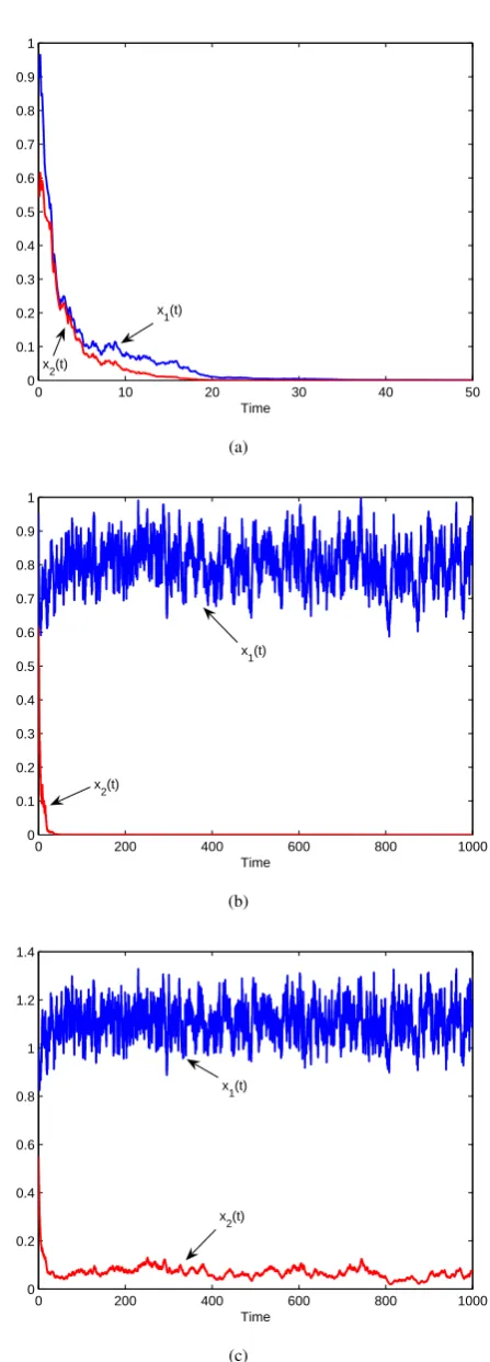
In Fig.2, the values of parameters are the same with these in Fig.1. Then according to Theorem 3, (7) holds. See Fig.2. In Fig.3(a), we choose α2₂₁ = 1.4, then by Theorems 4 and 5, bothx1 andx2 are extinct. See Fig.3(a). In Fig.3(b),

we choose α221 = 0.4, then in view of Theorems 4 and 5, x1 is weakly persistent in the mean and x2 is extinct. See

Fig.3(b). In Fig.3(c), we chooseα221= 0.04, then according

IAENG International Journal of Applied Mathematics, 46:4, IJAM_46_4_06

(10)

to Theorems 4 and 5, bothx1 andx2 are weakly persistent

in the mean. See Fig.3(c). By comparing Fig.1 and Fig.3(a), we can see that the more the random noises, the easier the species go to extinction.

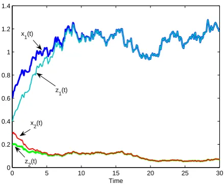
In Fig.4, the values of parameters are the same with these in Fig.1. Then according to Theorem 6, the model is globally asymptotically stable, see Fig.4.

0 200 400 600 800 1000 0

0.2 0.4 0.6 0.8 1 1.2 1.4

Time x₁(t)

[image:10.595.323.547.69.691.2]

x₂(t)

Fig. 1: Trajectories for model (3) with α2

11 = 0.2, α221 = 0, α2

12 = α222 = 0.1. This figure shows that the model is

stochastically bounded.

0 200 400 600 800 1000 −3

−2 −1 0 1 2 3

Time ln x₁(t)/ln t

[image:10.595.66.290.161.342.2]

ln x₂(t)/ln t

Fig. 2: Trajectories for model (3) with α2

11 = 0.2, α221 = 0,α2

12=α222= 0.1. This figure shows that (7) holds.

VII. CONCLUSIONS

In this paper, under the assumptions that r10 and r20

are affected by n independent standard Brownian motions, we have proposed and investigated a stochastic predator-prey populations model in polluted environments. We have established the existence, uniqueness and boundedness of the global positive solution. Sufficient conditions for extinction, non-persistence in the mean, weak persistence in the mean of the predator and prey populations have been established. The threshold between weak persistence in the mean and

0 10 20 30 40 50 0

0.1 0.2 0.3 0.4 0.5 0.6 0.7 0.8 0.9 1

Time x₁(t)

x₂(t)

(a)

0 200 400 600 800 1000 0

0.1 0.2 0.3 0.4 0.5 0.6 0.7 0.8 0.9 1

Time x₁(t)

x₂(t)

(b)

0 200 400 600 800 1000 0

0.2 0.4 0.6 0.8 1 1.2 1.4

Time x₁(t)

x₂(t)

(c)

Fig. 3: Solution of model (3). (a) shows that both x1 and x2 are extinct (α221 = 1.4); (b) shows that x1 is weakly

persistent in the mean and x2 is extinct (α221 = 0.4); (c)

shows that bothx1andx2are weakly persistent in the mean

(α2

21= 0.04).

IAENG International Journal of Applied Mathematics, 46:4, IJAM_46_4_06

[image:10.595.65.290.422.603.2]

(11)

0 5 10 15 20 25 30 0

0.2 0.4 0.6 0.8 1 1.2 1.4

Time x₁(t)

z₁(t) x₂(t)

[image:11.595.69.289.62.243.2]

z₂(t)

Fig. 4: Plot of two solution trajectories for model (3) with two sets of initial conditionsx1(0) = 0.6, x2(0) = 0.3 and z1(0) = 0.4, z2(0) = 0.2. This figure shows that model (1)

is globally asymptotically stable.

extinction for each species has been obtained. We have also studied the global asymptotic stability of the solution.

Our results indicate that the random interference of the prey populations x1 is neither conducive to the survival of x1 nor unfavorable tox2. However the random interference

of the predator populations x2 is only not conducive to the

survival of x2.

Our Theorems give some important and interesting bio-logical meanings. From Theorem 5 one can observe that if the two species have the same concentration of toxicant in the body, the ability for x1 to resist the toxicant is

stronger than that ofx2. Theorem 5 shows that if the average

growth rate r10 −r11⟨C0(t)⟩ of prey populations is less

than certain negative value for sufficiently large t, then both predator and prey populations are going to extinction. If the

average natural mortality rater20+ 0.5

n ∑

i=1

α2₂_i+r21⟨C0(t)⟩

of predator populations is larger than the maximum num-ber of average ingestion rate of prey populations [r10 −

0.5

n ∑

i=1

α21i −r11⟨C0⟩]/a11, then predator populations are

going to extinction. Our results also reveal that the more the random noises, the easier the species go to extinction. So in order to conserve biological diversity, we have the following solutions:

(i) To reduce the intensity of the the random noises. (ii) To reduce the number of the random noises. (ii) To reduce the input of the toxicant.

Some interesting problems deserve further investigation. In Theorem 2 and Theorem 7, the conditions have some limitations on aij. It is interesting to study whether these

conditions can be dropped. It is also of interest to investigate other multi-species systems (see e.g. [37], [38]).

REFERENCES

[1] T. G. Hallam, C. E. Clark and R. R. Lassider, “Effects of toxicant on population: a qualitative approach I. Equilibrium environmental exposure,”Ecological Modelling, vol. 8, no.3, pp. 291-304, 1983.

[2] T. G. Hallam, C. E. Clark and G. S. Jordan, “Effects of toxicant on population: a qualitative approach II. First Order Kinetics,”Journal of Mathematical Biology, vol. 109, no. 1, pp. 411-429, 1983.

[3] T. G. Hallam and J. L. Deluna, “Effects of toxicant on populations: a qualitative approach III. Environmental and food chain pathways,”

Journal of Theoretical Biology, vol. 109, no. 3, pp. 411-429, 1984. [4] T. G. Hallam and Z. Ma, “Persistence in population models with

demographic fluctuations,”Journal of Mathematical Biology, vol. 24, no. 3, pp. 327-339, 1986.

[5] Z. Ma. B. Song and T. G. Hallam, “The threshold of survival for systems in a fluctuating environment,”Bulletin of Mathematical Biology, vol. 51, no. 3, pp. 311-323, 1989.

[6] Z. Ma, G. Cui and W. Wang, “Persistence and extinction of a population in a polluted environment,”Mathematical Biosciences, vol. 101, no. 1, pp. 75-97, 1990.

[7] H. I. Freedman and J. B. Shukla, “Models for the effect of toxicant in single-species and predator-prey systems,”Journal of Mathematical Biology, vol. 30, no. 1, pp. 15-30, 1991.

[8] W. Wang and Z. Ma, “Permanence of populations in a polluted environment,”Mathematical Biosciences, vol. 122, no. 2, pp. 235-248, 1994.

[9] B. Buonomo, A. D. Liddo and I. Sgura, “A diffusive-convective model for the dynamics of population-toxicant intentions: Some analytical and numerical results,”Mathematical Biosciences, vol. 157, no. 2, pp. 37-64, 1999.

[10] P. D. N. Srinivasu, “Control of environmental pollution to conserve a population,”Nonlinear Analysis: Real World Applications, vol. 3, no. 3, pp. 397-411, 2002.

[11] J.He and K.Wang, “The survival analysis for a population in a polluted environment,”Nonlinear Analysis: Real World Applications, vol. 10, no. 3, pp. 1555–1571, 2009.

[12] H. Liu and Z. Ma, “The threshold of survival for system of two species in a polluted environment,”Journal of Mathematical Biology, vol. 30, no. 1, pp. 49-51, 1991.

[13] Z. Ma, W. Zong and Z. Luo, “The thresholds of survival for an n-dimensional food chain model in a polluted environment,”Journal of Mathematical Analysis and Applications, vol. 210, no. 2, pp. 440-458, 1997.

[14] J. Pan, Z. Jin and Z. Ma, “Thresholds of survival for an n-dimensional Volterra mutualistic system in a polluted environment,” Journal of Mathematical Analysis and Applications, vol. 252, no. 2, pp. 519-531, 2000.

[15] B. Liu, L. Chen and Y. Zhang, “The effects of impulsive toxicant input on a population in a polluted environment,”Journal of Biological Systems, vol. 11, no. 3, pp. 265-274, 2003.

[16] B. Liu, Z. Teng and L. Chen, “The effects of impulsive toxicant input on two-species Lotka-Volterra competition system,”International Journal of Information & Systems Sciences, vol. 1, no. 2, pp. 207-220, 2005.

[17] J. Jiao, W. Long and L.Chen, “A single stage-structured population model with mature individuals in a polluted environment and pulse input of environmental toxin,”Nonlinear Analysis: Real World Applications, vol. 10, no. 5, pp. 3073-3081, 2009.

[18] Z. Li and F. Chen, “Extinction in periodic competitive stage-structured Lotka-Volterra model with the effects of toxic substances,”Journal of Computational and Applied Mathematics, vol. 231, no. 1, pp. 143-153, 2009.

[19] R. M. May, Stability and Complexity in Model Ecosystems, USA: Princeton University Press, 2001.

[20] M.Liu and K.Wang, “Dynamics of a non-autonomous stochastic Gilpin-Ayala model,”Journal of Applied Mathematics and Computing, vol. 43, no. 1-2, pp. 351-368, 2013.

[21] T.C.Gard, “Stochastic models for toxicant-stressed populations,” Bul-letin of Mathematical Biology, vol. 54, no. 5, pp. 827–837, 1992. [22] M.Liu and K.Wang, “Survival analysis of stochastic single-species

population models in polluted environments,” Ecological Modelling, vol. 220, no. 9, pp. 1347-1357, 2009.

[23] M.Liu and K.Wang, “Persistence and extinction of a stochastic single-specie model under regime switching in a polluted environment,”

Journal of Theoretical Biology, vol. 264, no. 3, pp. 934–944, 2010. [24] K.Wang,Stochastic Models in Biomathematics, Beijing: Science Press,

2010.

[25] M.Liu, K.Wang and Q.Wu, “Survival analysis of stochastic competitive models in a polluted environment and stochastic competitive exclusion principle,”Bulletin of Mathematical Biology, vol. 73, no. 9, pp. 1969-2012, 2011.

[26] M.Liu and K.Wang, “Survival analysis of a stochastic cooperation system in a polluted environment,”Journal of Biological Systems, vol. 19, no. 2, pp. 183-204, 2011.

IAENG International Journal of Applied Mathematics, 46:4, IJAM_46_4_06

(12)

[27] M.Liu and K.Wang, “Persistence and extinction of a single-species population system in a polluted environment with random perturbations and impulsive toxicant input,”Chaos, Solitons & Fractals, vol. 45, no. 12, pp. 1541-1550, 2012.

[28] M.Liu and K.Wang, “Dynamics of a non-autonomous stochastic Gilpin-Ayala model,”Journal of Applied Mathematics and Computing, vol. 43, no. 1-2, pp. 351-368, 2013.

[29] Z.Geng and M.Liu, “Analysis of stochastic Gilpin-Ayala model in polluted environments,”IAENG International Journal of Applied Math-ematics, vol. 45, no. 2, pp. 128-137, 2015.

[30] X.R.Mao, G.Marion and E.Renshaw, “Environmental Brownian noise suppresses explosions in populations dynamics,”Stochastic Processes and their Applications, vol. 97, no. 1, pp. 95-110, 2002.

[31] S.Peng and X.Zhu, “Necessary and sufficient condition for comparison theorem of 1-dimensional stochastic differential equations,”Stochastic Processes and their Applications, vol. 116, pp. 370-380, 2006. [32] C.Ji, D.Jiang and N.Shi, ‘Analysis of a predator-prey model with

modified Leslie-Gower and Holling-type II schemes with stochastic perturbation,”Journal of Mathematical Analysis and Applications, vol. 359, pp. 482-498, 2009.

[33] I.Karatzas and S.E.Shreve,Brownian Motion and Stochastic Calculus, Berlin: Springer-Verlag, 1991.

[34] I.Barbalat, “Systems dequations differentielles d’osci d’oscillations nonlineaires,”Revue Roumaine de Mathematiques Pures et Appliquees, vol. 4, no. 2, pp. 267–270, 1959.

[35] D.J.Higham, “An algorithmic introduction to numerical simulation of stochastic differential equations.”SIAM Review, vol. 43, no. 3, pp. 525– 546, 2001.

[36] F.H.Shekarabi, M. Khodabin and K. Maleknejad, “The Petrov-Galerkin method for numerical solution of stochastic Volterra integral equations”,

IAENG International Journal of Applied Mathematics, vol. 44, no. 4, pp. 170-176, 2014.

[37] D. Jana, S. Chakraborty and N. Bairagi, “Stability, nonlinear oscil-lations and bifurcation in a delay-induced predator-prey system with harvesting,”Engineering Letters, vol. 20, no. 3, pp. 238-246, 2013. [38] M.Deng, “Analysis of a stochastic competitive model with regime

switching,”IAENG International Journal of Applied Mathematics, vol. 45, no. 4, pp. 373-382, 2015.