INDUCED CHARGE COMPUTATION METHOD Application in Monte Carlo simulations of inhomogeneous dielectric systems

Application in Monte Carlo simulations of inhomogeneous

dielectric systems

D. Boda1_{, D. Gillespie}2_{, B. Eisenberg}2_{, W. Nonner}3_{, D. Henderson}4 1_{Department of Physical Chemistry,}

University of Veszprém,

H–8201 Veszprém, P.O. Box 158, Hungary

2_{Department of Molecular Biophysics and Physiology,} Rush University Medical Center,

Chicago, Illinois 60612, USA

3_{Department of Physiology and Biophysics,} University of Miami School of Medicine, Miami, Florida 33101, USA

4_{Department of Chemistry and Biochemistry,} Brigham Young University,

Provo, Utah 84602, USA

Abstract In a recent publication we have introduced the induced charge computation

(ICC) method for the calculation of polarization charges induced on dielectric boundaries. It is based on the minimization of an appropriate functional. The resulting solution produces an integral equation that is transformed into a linear matrix equation after discretization. In this work, we discuss the effect of careful calculation of the matrix element and the potential by treating the polarization charges as constant surface charges over the various surface elements. The cor-rect calculation of these quantities is especially important for curved surfaces where mutual polarization of neighboring surface elements is considerable. We report results for more complex geometries including dielectric spheres and an ion channel geometry with a surface of revolution.

Keywords: Dielectric boundaries, Monte Carlo simulation, polarization charge

1.

Introduction

Understanding the behavior of physical systems containing many degrees of freedom requires considerable computational time unless we treat a cer-tain portion of the degrees of freedom as continuous response functions. These

19

response functions vary widely depending on the interactions they are intended to replace (electrostatic, dispersion, repulsion) and on the nonlocal nature of the medium (uniform homogeneous, inhomogeneous, anisotropic response func-tions). Because electrostatic interactions play a basic role in many fields such as molecular biology, quantum chemistry, electrochemistry, chemical engi-neering, and colloid chemistry (without any claim of this being a complete list), one of the most important response functions is the dielectric response of fast atomic and molecular motions. This procedure uses constitutive relations and macroscopic conservation laws and reduces to solving the Poisson’s equa-tion for source charges (which are the degrees of freedom treated explicitly) in an inhomogeneous dielectric medium characterized by a space dependent dielectric coefficient, ε(r).

One field where such a procedure is commonly used is the study of solva-tion of molecules. The solute (which can be treated quantum mechanically) is hosted in a cavity built in a dielectric continuum representing the solvent. This approach is called the polarizable continuum model (PCM) [1–3] which is studied by the apparent surface charge (ASC) method. This approach de-termines the surface charge induced on the surface of the cavity so that the appropriate boundary conditions are fulfilled at the boundaries. Using Green’s functions, the problem can be written in the integral equation formalism (IEF) [4–6], whose numerical solution results in a linear matrix equation. This ma-trix equation was first developed by Hoshi et al. [7] and named the boundary element method (BEM). Later Cammi and Tomasi [8, 9] adopted the method of Hoshi et al. and the group of Tomasi have developed several numerical proce-dures for the fast solution of the matrix equation using various iterative meth-ods [10]. The PCM has been extended to cases where the molecule is hosted in anisotropic solvents, ionic solutions, at liquid interfaces and metals [11]. There are a large number of studies using various BEM procedures including those implementing a linear interpolation across each boundary element to improve accuracy [12–18].

The most obvious example is the so called restricted primitive model (RPM) of electrolytes where the ions are represented as charges hard spheres, while the solvent is modelled as a dielectric continuum. Examples for inhomogeneous systems include electrochemical interfaces [19], semiconductor junctions [20], and cell membranes [21, 22].

A biologically crucial field where dielectric continuum models have a basic importance is ion channels embedded in the cell membrane. Several works have been published that use various methods to solve Poisson’s equation for channel-like geometries. These include interpolation methods using lookup tables to store discretized Green’s functions [23–27], BEM procedures [28– 30], generalized multipolar basis-set expansion of the Green’s function [31], and analytical solutions [30, 32–34]. The statistical mechanical methods also have a wide variety including the Poisson-Nernst-Planck (PNP) equation [32, 35, 36], Brownian dynamics (BD) simulations [23, 25, 26, 29, 31, 35, 36], the mean spherical approximation (MSA) for homogeneous fluids [37, 38], and Monte Carlo (MC) simulations [34, 39–42]. Special attention must be paid to the MC simulation works of Green and Lu [44–46] who developed a method to calculate dielectric boundary forces that practically equivalent to the BEM resulting in a matrix equation that corresponds to that developed by Hoshi et al. [7].

Ion channel studies motivated Allen et al. [47] who have developed an elegant variational formalism to compute polarization charges induced on di-electric interfaces. They solved the variational problem with a steepest descent method and applied their formulation in molecular dynamics (MD) simulations of water permeation through nanopores in a polarizable membrane [48–50]. Note that the functional chosen by Allen et al. [47] is not the only formal-ism that can be used. Polarization free energy functionals [51–53] are more appropriate for dynamical problems, such as macromolecule conformational changes and solvation [54–57].

boundary), and we have shown that our ICC method provides results in ex-cellent agreement with the simulations using the exact solution (on the basis of electrostatic image charges). Furthermore, we have reported results for the more general case of two parallel flat sharp boundaries (slab geometry) where the matrix is not diagonal.

The generalization of ICC method allows to impose arbitrary boundary con-ditions on various boundaries in the system [59]. Furthermore, a numerical approach to calculate the surface integrals appearing in the matrix elements has also been introduced [59]. The correct calculation of these integrals is es-pecially important in the case of curved surfaces; therefore, it is sometimes called “curvature correction”. In this work, we present the method of [58] supplemented by the “curvature corrections” introduced in [59] and we report results for more complex geometries than those considered in [58]. We show that “curvature corrections” are important not only for curved surfaces but also for the slab geometry if the slab is thin. We study the potential of a charge in a dielectric sphere and show results for the effective interaction between two charged dielectric spheres. We also show some preliminary results for a calcium channel that have a rotational geometry.

2.

Method

2.1

Variational formulation

Let us consider a discrete or continuous charge distributionρ(r)confined to a domainDof volumeV with a boundaryS. For the geometries considered in this work, the potential can be chosen to be vanishingly small onS. This makes the elimination of some surface terms possible. This does not mean that we impose zero potential on the boundary of the system. Instead, we use infinite systems (simply assuming that the system is infinite, or, in the case of simulation, applying periodic boundary condition), or, in the case of a finite simulation cell, we assume that the cell is large enough that the potential is small on the boundary in average. Nevertheless, the method has been gener-alized by Nonner and Gillespie [59] that makes it possible to directly impose arbitrary boundary conditions on the boundaries of the system. This general-ization is not considered in this paper.

P(r)produced by an electric fieldE(r)can be given as,

P(r) =ε0χ(r)E(r) =−ε0χ(r)∇ψ(r), (1) where χ(r) is the dielectric susceptibility. The dielectric susceptibility is space-dependent that characterizes an inhomogeneous dielectric in the domain

D. This corresponds to a local relative permittivityε(r) = 1 +χ(r). In gen-eral, this is a tensor, but in this work we restrict ourselves to a scalar relative permittivity (PandEhave the same directions). For the case of a bulk system, this quantity is called dielectric constant; in this work we use the term dielec-tric coefficient to emphasize that it is not constant in space. The polarization charge density induced by the source charge distribution is associated with the potential through,

ρpol(r) =−∇ ·P(r) =ε0∇ ·[χ(r)∇ψ(r)]. (2) Introducing the normalized versions of the source and the polarization charge densities,

g(r) =ρ(r) ε0

, (3)

and

h(r) =ρpol(r) ε0

, (4)

Poisson’s equation can be given as,

∇2ψ(r) =−[g(r) +h(r)], (5) and the corresponding functional [47] is,

I[ψ] =1 2

D

∇ψ· ∇ψdr−

D ψ

g+1

2∇ ·(χ∇ψ)

dr. (6)

In order to expressI[ψ]as a functional of the polarization charge density, the potential is also split into the “external” and the “induced” parts which are expressed in terms ofg(r)andh(r)with the help of the Green’s function as,

ψ(r) = ψe(r) +ψi(r) =

=

D

G(r−r′)g(r′)dr′+

D

G(r−r′)h(r′)dr′, (7)

where the Green’s function satisfies,

withδ(r−r′)being the Dirac delta function. Substituting Eq. (7) into Eq. (6), the functional can be given as a function of g(r), h(r), and ψe(r), e. g.

I =I[g, h, ψe]. The task is to determine the polarization charge densityh(r) for a given external charge densityg(r)that satisfies Eq. (5), or, equivalently, minimizesI[g, h, ψe]. Determiningh(r)for a fixedg(r)is equivalent to mini-mizing theh-dependent part of the functionalI[g, h, ψe], which is denoted by

I2[h]. Allen et al. [47] showed that the extremum condition,

δI2[h]

δh(r) = 0, (9)

leads back to the constitutive relation in Eq. (1), that the extremum is a min-imum, and that the value ofI[h]at the minimum reduces to minus the elec-trostatic energy. Allenet al. [47] solved the variational problem (after dis-cretization) with a steepest descent method. In our previous work [58], we have proposed a different route that results in the integral equation,

h(r)ε(r)−

D

h(r′)∇rε(r)· ∇rG(r−r

′

)dr′=

=∇rε(r)· ∇rψe(r)−[ε(r)−1]g(r). (10) Discretizing the central equation (Eq. (10)) of the ICC method leads to a matrix equation. In this work, we focus on the case of sharp dielectric bound-aries, therefore, we will show the details of discretization for that case. To our knowledge, this equation for the general caseε(r)has not been derived previ-ously. Recently, Frediani et al. [11] has reported an integral equation for the case of a molecule solvated at a diffuse interface between two fluid phases (liq-uid/liquid or liquid/vapor). Their interface is described by a dielectric profile

ε(z)that is a continuous function of thezcoordinate, while the charge distrib-ution of the molecule is placed in a cavity formed in the diffuse interface. An integral equation has been developed by Frediani et al. by finding the appropri-ate Green’s function through certain integral operators. The resulting equation is similar to Eq. (10), but is less general.

2.2

Discrete, point source charges

When the source charges are point charges in discrete locations, the source charge density is given by

g(r) = e ε0

k

zkδ(r−rk), (11)

around each point chargekis localized at its positionrk. Assuming that the dielectric is locally uniform around the source chargezkewith dielectric co-efficientε(rk), the magnitude of the induced charge is−zke[ε(rk)−1]/ε(rk) [60]. Therefore, the contribution to hfrom the induced charges around the source charges is,

h′

(r) =−e

ε0

k

zk

ε(rk)−1

ε(rk)

δ(r−rk). (12)

Let us consider the source point chargesg(r)and the induced chargesh′

(r) lo-calized on them together; and let us denote the sum of these two terms byg(r) hereafter. In other words, we moveh′

(r)from the group of induced charges to the group of source charges. Accordingly, the electric potential raised byh′

(r) also contributes to the potential of the source point charges; the sum of the two potentials is denoted byψehenceforth. It can be shown that for the resulting potential,

∇2_ψ

e(r) =−g(r) +h′(r)=−

e ε0

k

zk

ε(rk)

δ(r−rk), (13)

applies from which this potential is expressed as,

ψe(r) =

e 4πε0

k

zk

ε(rk)|r−rk|

. (14)

The dielectric coefficientε(rk)at the place of chargekappears in the denomi-nator. This corresponds to a dielectric screening that is conventionally used in various descriptions of electrolytes where the solvent is interpreted as a dielec-tric continuum background (for instance, in the Debye-Hückel theory, in the Gouy-Chapman theory, or in the RPM of electrolyte solutions).

Substituting the redefinedg(r)andψe(r)into Eq. (10), we obtain,

h(r)ε(r)−

D

h(r′)∇rε(r)· ∇rG(r−r′)dr′=∇rε(r)· ∇rψe(r), (15) whereh(r)refers solely to the induced charges other thanh′

(r).

There-fore, in the simulations, we assume that the interior of the ion has the same dielectric coefficient as the surrounding medium. For the same reason, we as-sume that the ions move in regions of constant dielectric coefficient, namely, they do not overlap with dielectric boundaries and they are not displaced from one dielectric domain to another. In this work, we will show results for the cases where the interior of an ion has different dielectric coefficient than that of the surrounding medium.

2.3

Sharp dielectric boundaries

In the special case of sharp dielectric boundaries the dielectrics is sepa-rated into domains of uniform dielectric coefficients. The dielectric coefficient jumps from one value to another along a boundary. Let us denote the surface of the dielectric boundaries byB. Then the induced charge is a surface charge on the dielectric interfaces (if the induced charges around the source charges are not considered), and the volume integral in Eq. (15) becomes a surface integral over the surfaceB,

h(s)ε(s)−∆ε(s)

B

h(s′)∇sG(s−s

′

)·n(s)ds′= ∆ε(s)∇ψe(s)·n(s), (16) where the dielectric coefficientε(s)on the boundary is defined to be the arith-metic mean of the two dielectric coefficients on each side of the boundary. Furthermore, the dielectric jump∆ε(s)is the difference of the two dielectric coefficients on each side of the boundary in the direction of the local unit nor-mal of the surfacen(s).

To solve Eq. (16) numerically, the surface Bmust be discretized; specif-ically, each discrete surface elementBα of Bis characterized by its center-of-masssα, area aα, unit normal nα = n(sα), value of the mean dielectric coefficientεα =ε(sα), and value of the dielectric jump∆εα = ∆ε(sα). Due to the assumption of the vanishingly small potential onS, the Green’s function simply is,

G(s−s′) = 1

4π|s−s′_|. (17)

Also, since the density of the discrete point charges is given, the resulting po-tentialψe is known from Eq. (14). Of course,∇sG(s−s′)and∇ψe(s)are also known. The otherwise continuous surface charge densityh(s)is then discretized into certain constant valueshα =h(sα)taken on the surface ele-mentBα.

assumption thathβis constant overBβ, we obtain for a givenα that,

β

hβ

εβδαβ−∆εα

B_β

∇sαG(sα−sβ)·nαdsβ

=

= ∆εα∇ψe(sα)·nα, (18) whereδαβis the Kroneckerδ. This can be rewritten in a matrix form as,

Ah=c, (19)

where each element of the matrixAis given by the expression in square bra-ckets,

Aαβ=εβδαβ−∆εαIαβ, (20)

whereIαβdenotes the integral in Eq. (18). Each element of the column vector his given byhβand each element of the column vectorcis given by the right hand side of Eq. (18),

cα= ∆εα∇ψe(sα)·nα. (21)

For the calculation of the integralIαβ, there are two levels of approximation to interpret the charge on a surface element. The first route is to consider the surface charge as a point charge of magnitudehβaβ localized atsβ. We call this approach the point charge(PC) approximation. In this case the integral reduces to an interaction term between point charges,

Iαβ=∇sαG(sα−sβ)·nαaβ (22)

forβ =αand0otherwise (an induced point charge does not polarize itself). This approach was used in our previous work [58], where we tested the method on planar dielectric interfaces.

On the higher level of approximation, the induced charge on theβth surface element is considered as a surface charge with the constant value hβ. This approach, which we call the surface charge(SC) approximation, was intro-duced in [59]. The main difference is geometrical: the values of the integrals in Eq. (18) do not depend on charges, they depend only on the geometry of the dielectric boundary surfaces and the way they are discretized. The integral represents the polarization of the induced charges on the surface elementBβ by the induced charge atsα. Practically, this approach means that we have to evaluate the surface integralsIαβ. This is a numerical problem; a procedure to solve it was proposed in [59]. We parametrize the two-dimensional surface

Bβ by two variablesuandv. There is a transformation that convertsuand

Therefore, bothG(sα−sβ)andn(sα)can be expressed in terms of the new parameters: G(uα, vα, uβ, vβ)andn(uα, vα). Let us discretize the βth sur-face element into subelements by evenly dividing the variablesuβandvβ into subintervals of widths∆uβand∆vβ. Then, the integral can be calculated as,

Iαβ=

k

l

∇αG(uα, vα, uβ,k, vβ,l)·n(uα, vα)a(uβ,k, vβ,l) ∆uβ∆vβ,

(23) where a(uβ,k, vβ,l) denotes the area element and(uβ,k, vβ,l)gives the center of thek, lth subelement of theβth surface element. Also, care must be taken to ensure thatuα =uβ,kandvα=vβ,l.

It has been realized before that the convergence of the results with increas-ing the resolution of the grid is poor usincreas-ing the PC approximation. A curvature correction was used by many workers [1, 3, 7, 23, 24], where an empirical parameter was built into the diagonal elements of the matrix (for reviews, see [18, 61]). Instead of this uncertain parameter, it is more appropriate to evaluate the integrals numerically. In our SC approximation, the integrals are computed by assuming that the surface charge is constant within a surface element. A higher level approximation was used in several works [12–18] where the sur-face charge within a sursur-face element is interpolated from the sursur-face charges in the neighboring tiles. Recently, Chen and Chipman [18] have proposed a linear interpolation method using a triangulation of the surface. The sample points (sα) are the corners of the triangles, and the integrals over the triangles are evaluated by interpolating the surface charge inside a triangle from those at the three corners. The development of a similar interpolation method for our parametrization procedure using theu, vparameters is under way.

The evaluation of the integrals in the SC approximation is quite time con-suming. Nevertheless, the speed of filling and inverting the matrix is not an issue in computer simulations if the geometry of the dielectric boundaries does not change during the simulation. Thus, the inverse ofA(or any factorization ofA) need only be computedoncefor a given geometry and dielectric pro-file. The calculation ofIαβ by subdiscretizing the surface elements does not increase the sizeof the matrix, it only influences the fill timeof the matrix, which is also performed once at the beginning of a simulation.

2.4

Calculation of the energy

In an MC simulation the essential quantity is the change in the energy of the system in an MC step. The MC step is normally a stochastic particle displace-ment, chosen from a uniform distribution, but biased moves are also possible [62–65]. Some details of our MC simulations will be given in the Results section, here we give the procedure with which the electrostatic energy is cal-culated in the framework the ICC method. We assume that the source charges are point charges and that the dielectric boundaries are sharp as described in the preceding two subsections.

The electrostatic energy can be split into two parts. The source charge – source charge interaction energy is,

We=

1 2

j

ezjψe(rj), (24)

where the electrostatic potential of the source point charges is given by Eq. (14). The source charge – induced charge interaction is given by,

Wi=

e 8π j zj B h(s)

|s−rj|

ds. (25)

After discretization, as in the case of filling the matrix, we have two choices in the calculation of the above integral. In the PC approximation the integral becomes a sum of point charge – point charge interactions,

Wi=

e 8π j zj β

hβaβ

|sβ−rj|

. (26)

In the above equations, the indicesjandβrange over the source point charges and the surface elements, respectively. In the SC approximation the integral expresses a point charge – surface charge interaction,

Wi=

e 8π j zj β hβ B_β ds

|s−rj|

. (27)

ions with a finite diameter and the ion centers (where the source charges are located) cannot approach the surface closer than the half of the ionic diameter, this problem does not arise in our simulations.

In a usual MC simulation we use single particle movements, namely, only one particle is displaced in an MC step. This fact and the linearity of the matrix equationAh=cmake it possible to decrease the computation time of the en-ergy change ∆W. This is because the distances between particles that are not moved do not change in the MC step and the distances between these particles and the surface elements are also unchanged. Storing the intermolecular dis-tances in an array, the computational burden can be decreased by saving time consuming square roots. The details can be found in [58].

It is important to note that in our simulations we assume that the ions do not cross the dielectric boundaries. If an ion were to cross a dielectric bound-ary in the MC step, the energy of interaction of the ion with the two different dielectrics (that corresponds to the solvation energies) must be included. Cal-culating such energies is difficult. Instead, empirical parameters describing this energy difference might be included in the calculation as in our previous work [34] where we studied the selectivity of a calcium channel where the di-electric coefficient of the selectivity filter was different from that of the bulk electrolyte. Nevertheless, estimating such empirical parameters is still prob-lematic. Therefore, as a first approximation, we avoid this problem and assume that the dielectric boundaries act as hard walls and the ions cannot leave their host dielectrics.

3.

Results

3.1

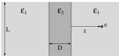
Planar geometry

ε

ε

ε

z

D

e

L

Figure 1. The slab geometry.

two physical points in the simulation cell including points on the boundary surfaces (sβ). Here we show results only for one source point charge.

Nev-ertheless, to remain in connection with simulations, we use two square walls of dimensionsL×L, although using circular walls with the charge above the

center is also possible. According to periodic boundary conditions, the grids on the surface of the two walls are constructed by evenly dividing them into square elements of width∆x(withL/∆xbeing an integer). This means that the surface elements are parametrized by the xandy variables (u = xand v =y). The value of∆x, namely the fineness of the grid, is a crucial point of the calculation (it was discussed in [58] in detail). Briefly,∆xmust be small enough compared to the closest approach of a charge to the surface. Further-more, the dimensions of the simulation cell have to be large enough, which is a usual criteria in computer simulations.

0.5 1 1.5 2 z / ∆x

0.4 0.8 1.2

Wi

(z)/kT

0.4 0.8 1.2

Wi

(z)/kT

0.4 0.8 1.2

Wi

(z) / kT

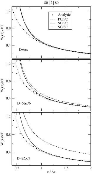
Analytic PC/PC SC/PC SC/SC 80 | 2 | 80

D=∆x

D=5∆x/6

D=2∆x/3

Figure 2. The polarization energyWiof a single charge of magnitudeeas a function of the distance of the charge from the slab for different slab widths. The dielectric coefficients of the slab geometry areε1= 80;ε2 = 2;ε3 = 80. The polarization energy is normalized bykT

whereT= 300K. The ICC curves as obtained from different approaches (PC/PC, SC/PC, and SC/SC; the explanation of the abbreviations can be found in the main text) are compared to the analytical solution [66].

form of infinite series. Here, we use the formulas given by Allen and Hansen [66].

We consider three possibilities that differ whether we use the PC or the SC approximation in the calculation of Iαβ and/or Wi:

(2) Using Eq. (23) for the calculation of the matrix element and Eq. (26) for the calculation ofWimeans that the SC approximation is used only to fill the matrix (SC/PC).

(3) If we use Eq. (23) for the calculation of the matrix element and Eq. (27) for the calculation ofWi, the SC approximation is used in both cases (SC/SC). As mentioned before, using Eq. (27) significantly slows the simulation.

These notations will also be used in subsequent subsections.

r

o e

R ε

ε

1

2

d (a)

∆φ ∆θ

(b)

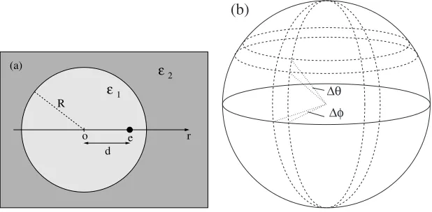
Figure 3. (a) The geometry of a dielectric sphere of dieletric coefficientε1embedded in a

mediun of dielectric coefficientε2with a source point charge within the sphere. (b) The grid on

the surface of a sphere is constructed by evenly dividing the spherical coordinatesφandθinto subintervals of widths∆φand∆θ.

3.2

One dielectric sphere

A dielectric sphere of dielectric coefficientε1embedded in an infinite di-electric of permittivityε2is an important case from many points of view. The idea of a cavity formed in a dielectric is routinely used in the classical theo-ries of the dielectric constant [67–69]. Such cavities are used in the studies of solvation of molecules in the framework of PCM [1–7] although the shape of the cavities mimic that of the molecule and are usually not spherical. Di-electric spheres are important in models of colloid particles, electrorheological fluids, and macromolecules just to mention a few. Of course, the ICC method is not restricted to a spherical sample, but, for this study, the main advantage of this geometry lies just in its spherical symmetry. This is one of the simplest examples where the dielectric boundary is curved; and an analytic solution is available for this geometry in the form of Legendre polynomials [60]. In the previous subsection, we showed an example where the SC approximation is important while the boundaries are not curved. As mentioned before, using the SC approximation is especially important if we consider curved dielectric boundaries. The dielectric sphere is an excellent example to demonstrate the importance of “curvature corrections”.

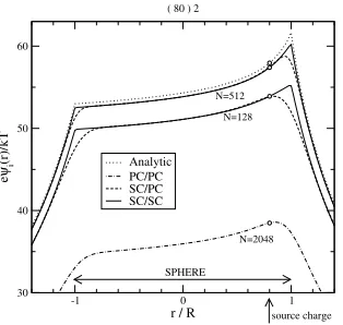
-1 0 1

r / R

30 40 50 60

e

ψi

(r)/kT Analytic

PC/PC SC/PC SC/SC

( 80 ) 2

SPHERE

source charge N=512

N=128

N=2048

Figure 4. The potential of the induced chargeseψi(r)/kTas a function ofralong the line crossing the center of the sphere and the source charge. The ICC curves as obtained from dif-ferent approaches (PC/PC, SC/PC, and SC/SC) are compared to the analytical solution obtained from a series expansion of Legendre polynomials [60].

spherical symmetry, the surface of the sphere is parametrized by the spherical coordinates (u=θandv=φ). The geometry is shown in Fig. 3a, while the corresponding grid is illustrated in Fig. 3b. A source charge is placed inside the sphere in a distanced= 0.8Rfrom the center of the sphere, whereRis the radius of the sphere. Fig. 4 shows the potential produced by the polariza-tion charges induced by the source charge on the surface of the sphere. The dimensionless potentialeψi/kT is plotted as a function ofr/R, whereris the distance from the center of the sphere along the line through the center and the source charge. The positive direction shows from the center to the source charge. In the case of the PC/PC approach there is a large difference between the analytic and the ICC solutions even for a very large number of surface elementsN = 2048(dot-dashed line). If we use the SC approximation to cal-culate the matrix elements (SC/PC), the agreement with the analytic solution becomes much better, but near the surface of the sphere the ICC curves (dashed lines) fail to reproduce the kinks in the analytic curve (dotted lines). Increasing the number of surface elements (fromN = 128toN = 512) the ICC curves approach the analytic curve. Using the SC/SC approach, the behavior of the ICC curves becomes satisfactory even in the vicinity of the boundary of the sphere (solid lines).

It is important to determine the centers of the surface elements correctly. If we parametrize the area elementαby the variablesuandvthen the coordinates of the center are calculated as,

uα=

Bαu a(u, v)dudv

B_αa(u, v)dudv

, (28)

and similarly for vα, wheres = (uα, vα)is the center of the tile [59]. The centers of the subelements should be calculated similarly. If we determine the center by simply taking the centers of the∆uαand∆vαintervals instead of the above weighted average, we introduce a small error into our calculation. For the example of the one dielectric sphere, the polarization energy (Wi/kT =

eψi(d)/kT denoted by open circles in Fig. 4) is 57.4 if we calculatescorrectly from Eq. (28) (using 512 tiles), and 57.074 otherwise. The analytical value is 57.9616. Although it is small, this error might be important as in the case of the two spheres in the next subsection.

3.3

Two dielectric spheres

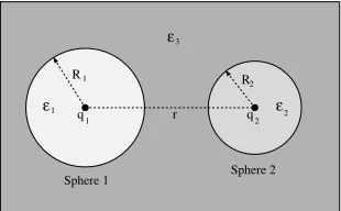
investigated by Allen and Hansen [70] who used their variational approach to calculate the effective interaction between charges within dielectric cavities. For a few special cases, they have developed solutions for the problems in the form of series expansions without using a grid. The general situation for spherical cavities can be seen in Fig. 5. Two dielectric spheres of radiiR1 andR2are immersed in a dielectric of dielectric coefficientε3. The dielectric coefficients in the spheres areε1 andε2. The distance of the centers of the spheres isr. Point charges of magnitudesq1andq2are placed at the centers of Sphere 1 and 2, respectively.

q r q

R

2 2

1

R1

ε ε

ε

1 2

3

Sphere 1 Sphere 2

Figure 5. The geometry for two charges within dielectric spheres.

If the dielectric is homoegeneous (ε1 = ε2 = ε3), the interaction poten-tial between the charges is the Coulomb potenpoten-tial divided byε3. Introducing the effective dielectric coefficientεeff(r)[70], the interaction potential can be written in the form of the Coulomb potential by

Vint(r) = q1q2

4πε0εeff(r)r

(29)

for the case where dielectric boundaries are present. The interaction potential is defined by the difference,

Vint(r) =W(r)−W(∞), (30)

whereW(∞)is the energy of the system when the spheres are infinitely far from each other. This term is the interaction energy between the ions and the polarization charges induced by the charges on their own spheres. This is an “intramolecular” term, whileVint(r)is an “intermolecular” term which goes to zero increasing the distance of the spheres. For the former term an analytical expression exists,

W(∞) = ε1−ε3

8πε0ε1ε3

q2 1

R1

+ ε2−ε3 8πε0ε2ε3

q2 2

R2

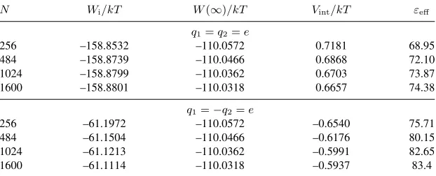
Figure 6 shows results for the caseε1 =ε2= 1,ε3= 80,R =R1 =R2 with charges of the opposite (q1=−q2=e, Fig. 6a) and the same (q1=q2=

e, Fig. 6b) sign. This corresponds to two ions solvated in water, where the ions are modelled as vacuum spheres with point charges in the center. When the dis-tance of the spheres is large, the solution of the problem converges to the case of point charges with the polarization charges localized on them (discussed in Sec. 2.2). In this limit,εeff(r)→ε3forr→ ∞. We have calculated the en-ergy of the two sphere systems forr/R= 2.25, 2.5, 2.75, and 3 using various numbers of surface elements (N = 256, 484, 1024, and 1600). The effective dielectric coefficient is plotted as a function of1/N(open circles). In the limit of “infinitely fine” grid (1/N →0), the analytical results obtained from Figs. 5b and 5d of the paper of Allen and Hansen [70] are also shown (filled circles). Increasing the number of tiles, our results converge to the analytical data.

76 78 80 82 84

εeff

(r)

0 0.002 0.004 0.006 0.008

1/N

68 70 72 74 76 78

εeff

(r)

r=3R r=2.75R

r=2.5R

r=2.25R r=2.25R r=2.5R r=2.75Rr=3R

(a)

(b) q₁=-q₂

q₁=q₂

Figure 6. The effective dielectric coefficient as a function of1/N, whereNis the number of tiles. Results are shown for charges of opposite (a) and equal (b) sign for different distances of the spheres. The filled circles are analytical results [70].

The convergence is quite slow, however. To explain this, the energies ob-tained for two specific cases with different fineness of grid are tabulated in Tab. 1. The small value ofVintis obtained from the sum of three large quan-tities: Vint = We +Wi −W(∞). For this reason, a small error inWi or

in-Table 1. The various energies calculated for distancer/R = 2.25for equal and opposite charges. The direct interaction between the charges isWe/kT =±_{49.5140. The analytical}

value for the energy of separated spheres isW(∞_)/kT=−_{110.0139calculated from Eq. (31).}

The literature data for the effective dielectric coefficient isεeff ∼_{74.7and 84.3 for equal and}

opposite charges, respectively.

N Wi/kT W(∞_{)/kT Vint/kT εeff}

q1=q2=e

256 –158.8532 –110.0572 0.7181 68.95

484 –158.8739 –110.0466 0.6868 72.10

1024 –158.8799 –110.0362 0.6703 73.87

1600 –158.8801 –110.0318 0.6657 74.38

q1=−_q2=e

256 –61.1972 –110.0572 –0.6540 75.71

484 –61.1504 –110.0466 –0.6176 80.15

1024 –61.1213 –110.0362 –0.5991 82.65

1600 –61.1114 –110.0318 –0.5937 83.4

teraction between the charges (We) is screened by a corresponding term raised by the polarization charges (Wi−W(∞)). Note that for W(∞)the value obtained from our numerical method was used instead of the analytical value because the same numerical errors appear in bothWe andW(∞)which can-cel each other. Using the analytical value forW(∞)results in a considerable overestimation ofεeff.

In these two subsections, simple calculations for systems containing dielec-tric sphere(s) have been presented. Simulations for the distribution of ions around and within dielectric sphere(s) are under way.

3.4

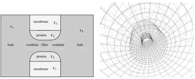
Ion channel geometry

study, the filter is embedded in a membrane (Fig. 7a). The two baths are connected to the filter through two cone shaped vestibules at the entries of the filter (these vestibules were absent in our earlier studies). The system has a rotational symmetry: the surfaces in the simulation cell form a surface of revolution around the centerline of the pore.

membrane 3

ε

vestibule filter vestibule

protein

membrane protein bath

ε ε ε

ε₁

2 2

3

bath

ε

1 1

Figure 7. (a) The simulation cell for the ion channel geometry. (b) Illustration of the method

to construct the grid on the dielectric boundary surfaces.

The dielectric coefficient was uniform (ε= 80) in our previous studies [39– 42]. In this work, we present some MC results for the case where we allow var-ious regions in the system to have different dielectric coefficient. Specifically, the membrane, the protein, and the electrolyte solution in which the ions move have dielectric coefficients ε3 = 2, ε2 = 20, and ε1 = 80, respectively. The dielectric boundary surfaces that appear in the simulation cell have dif-ferent geometries. Consequently, difdif-ferent u, v parameters are used for these surfaces. Due to the rotational symmetry, the variable φ is one of the parame-ters in all cases. The other parameter depends on the geometry of the various regions which are: (1) filter/protein and (2) protein/membrane boundaries – cylinders with z the second parameter, (3) vestibule/protein boundary – a cone

shaped surface with a spherical curvature (an appropriateθangle parametrize the curvature), and (4) bath/membrane boundary – planes perpendicular to the

z-axis, the other parameter isrwhich is the distance from the rotational axis. The grid we constructed is illustrated in Fig. 7b; the grid is finest inside the filter (where important things happen) and it becomes coarser farther from the filter.

length (that equals the width of the membrane) is 30 Å. This means that the curvature radius of the vestibules is 10 Å.

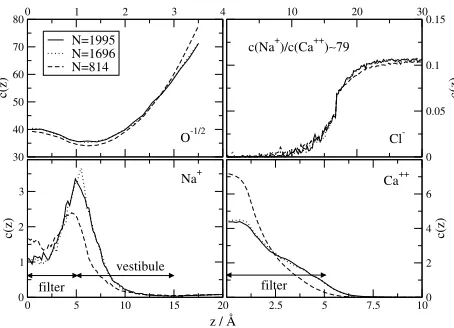
There are 8 half charged oxygen ions (with diameters 2.8 Å) in the filter representing the 4 unprotonated structural groups of the EEEE locus of the calcium channel. These ions are assumed to be mobile inside the filter but they are restricted to the filter. There are 100 sodium and 100 chloride ions (diameters 1.9 and 3.62 Å) in the system in appropriate numbers to obtain a 0.1 M NaCl solution in the bath. There are also 2 calcium ions (diameter 1.98 Å). Thus, the whole simulation cell is electroneutral.

0 1 2 3 4

30 40 50 60 70 80

c(z)

N=1995 N=1696 N=814

10 20 30

0 0.05 0.1 0.15

c(z)

0 5 10 15 20

0 1 2 3

c(z)

2.5 5 7.5 100 2 4 6

c(z)

O-1/2 Cl

-Na+ Ca++

z / Å

c(Na+)/c(Ca++)∼79

filter

vestibule

filter

Figure 8. The concentration profiles for the various ionic species as obtained from MC

simu-lations applying grids of different resolutions. The system is symmetric for the center plane of the membrane, so the results obtained for the left and right sides are averaged.

We present results of 3 simulations which differ from each other only in the resolution of the grid. The widths of the surface elements in the filter are 1.43, 1, and 0.91 Å, which correspond to total number of tilesN =814, 1760, and 1995, respectively. The lengths of the simulations are 886 000, 339 000, and 308 000 MC cycles, respectively. Besides the usual particle displacements, biased particle exchanges between the channel and the baths were applied (for details, see [41, 42]).

ions tend to accumulate in the center of the filter, while the Na+_{ions are rather} positioned at the entries of the filter and in the vestibules. This result clearly shows the importance of dielectric boundaries.

For this work, the important aspect of our simulation is the dependence of the results on the resolution of the grid. It is seen that our results converge as the number of surface elements is increased. ForN= 814the curves are quite different from those obtained for N = 1696and 1995 although the qualita-tive behavior is the same. The curves obtained for the two better resolutions differ from each other only in minor details. This is in accordance with our earlier findings which showed that we can obtain accurate results from simu-lations if the dimensions of the surface elements are smaller than the closest approach of the ions to the surfaces. The SC/PC approximation was used in our simulations.

4.

Summary

We have presented the ICC method with developments in which the polar-ization charges are treated as surface charges with a constant value inside a boundary element (SC approximation). We have discussed the effect of using the SC approximation to calculate the matrix elements and polarization energy for various geometries. It was shown that this approach is important not only for curved dielectric boundaries but also for flat boundaries if the are close to each other. On the examples of dielectric spheres, it was shown that using the SC approximation (or “curvature corrections”) is especially important for curved surfaces. If the geometry of dielectric interfaces does not change during a simulation, the method can efficiently been used in computer simulations, as our results for an ion channel geometry do show.

References

[1] Miertus, S., Scrocco, E., and Tomasi, J.Chem. Phys., 1981,55, p. 117. [2] Tomasi, J., and Persico, M.Chem. Rev., 1994,94, p. 2027.

[3] Klamt, A., and Schüürmann, G.J. Chem. Soc. Perkin. Trans., 1993,2, p. 799. [4] Mennucci, B., Cancès, E., and Tomasi, J.J. Phys. Chem. B, 1997,101, p. 10506. [5] Mennucci, B., and Cancès, E.J. Math. Chem., 1998,23, p. 309.

[6] Mennucci, B., Cammi, R., and Tomasi, J.J. Chem. Phys., 1998,109, p. 2798. [7] Hoshi, H., Sakurai, M., Inoue, Y., and Chûjô, R.J. Chem. Phys., 1987,87, p. 1107. [8] Cammi, R., and Tomasi, J.J. Chem. Phys., 1994,100, p. 7495.

[9] Cammi, R., and Tomasi, J.J. Chem. Phys., 1994,101, p. 3888.

[10] Pomelli, C.S., Tomasi, J., and Barone, V.Theor. Chem. Acc., 2001,105, p. 446, (and references therein).

[12] Zauhar, R.J., and Morgan, R.S.J. Comput. Chem., 1988,9, p. 171.

[13] Yoon, B.J., and Lenhoff, A.M.J. Comput. Chem., 1990,11, p. 1080.

[14] Juffer, A.H., Botta, E.F.F., van Keulen, B.A.M., van der Ploeg, A., and Berend-sen, H.J.C.J. Comp. Phys., 1991,97, p. 144.

[15] Fox, T., Rösch, N., and Zauhar, R.J.J. Comput. Chem., 1993,14, p. 253. [16] Liang, J., and Subramaniam, S.Biophys. J., 1997,73, p. 1830.

[17] Bordner, A.J., and Huber, G.A.J. Comput. Chem.24, 353 (2003).

[18] Chen, F., and Chipman, D.M.J. Chem. Phys., 2003,119, p. 10289.

[19] Torrie, G.M., Valleau, J.P., and Patey, G.N.J. Chem. Phys., 1982,76, p. 4615. [20] Jacoboni, C., and Luigi, P. (1989).The Monte Carlo Method for Semiconductor Device

Simulation. New York: Springer Verlag.

[21] Parsegian, V.A.Nature (Lond.), 1969,221, p. 844.

[22] Neumcke, B., and Läuger, P.Biophys. J., 1969,9, p. 1160.

[23] Hoyles, M., Kuyucak, S., and Chung, S.-H.Phys. Rev. E, 1998,58, p. 3654.

[24] Hoyles, M., Kuyucak, S., and Chung, S.-H.Comput. Phys. Commun., 1998,115, p. 45.

[25] Chung, S.-H., Hoyles, M., Allen, T., and Kuyucak, S.Biophys. J., 1998,75, p. 793.

[26] Chung, S.-H., Allen, T., Hoyles, M., and Kuyucak, S.Biophys. J., 1999,77, p. 2517.

[27] Graf, P., Nitzan, A., Kurnikova, M., and Coalson, R.J. Phys. Chem. B, 1997,101, p. 5239.

[28] Levitt, D.G.Biophys. J., 1978,22, p. 209;ibid, 1978,22, p. 221.

[29] Corry, B., Allen, T., Kuyucak, S., and Chung, S.-H.Biophys. J., 2001,80, p. 195.

[30] Ba¸stuˆg, T., and Kuyucak, S.Biophys. J., 2003,84, p. 2871.

[31] Im, W., and Roux, B.J. Chem. Phys., 2001,115, p. 4850.

[32] Schuss, Z., Nadler, B., and Eisenberg, R.S.Phys. Rev. E, 2001,64, p. 036116. [33] Nadler, B., Hollerbach, U., and Eisenberg, R.S.Phys. Rev. E, 2003,68, p. 021905.

[34] Boda, D., Varga, T., Henderson, D., Busath, D.D., Nonner, W., Gillespie, D., and Eisenberg, B.Mol. Sim., 2004,30, p. 89.

[35] Moy, G., Corry, B., Kuyucak, S., and Chung, S.-H.Biophys. J., 2000,78, p. 2349. [36] Corry, B., Kuyucak, S., and Chung, S.-H.Biophys. J., 2000,78, p. 2364. [37] Nonner, W., Catacuzzeno, L., and Eisenberg, B.Biophys. J., 2000,79, p. 1976.

[38] Nonner, W., Gillespie, D., Henderson, D., and Eisenberg, B.J. Phys. Chem. B, 2001, 105, p. 6427.

[39] Boda, D., Busath, D.D., Henderson, D., and Sokołowski, S.J. Phys. Chem. B, 2000, 104, p. 8903.

[40] Boda, D., Henderson, D., and Busath, D.D.J. Phys. Chem. B, 2001,105, p. 11574. [41] Boda, D., Henderson, D., and Busath, D.D.Mol. Phys., 2002,100, p. 2361.

[42] Boda, D., Busath, D.D., Eisenberg, B., Henderson, D., and Nonner, W.Phys. Chem. Chem. Phys., 2002,4, p. 5154.

[43] Gillespie, D., Nonner, W., and Eisenberg, R.S. J. Phys.: Condens. Matt., 2002,14,

p. 12129.

[45] Green, M.E., and Lu, J.J. Phys. Chem. B, 1997,101, p. 6512.

[46] Lu, J., and Green, M.E.J. Phys. Chem. B, 1999,103, p. 2776.

[47] Allen, R., Hansen, J.-P., and Melchionna, S.Phys. Chem. Chem. Phys., 2001,3, p. 4177.

[48] Allen, R., Melchionna, S., and Hansen, J.-P.Phys. Rev. Letters, 2002,89, p. 175502.

[49] Allen, R., Melchionna, S., and Hansen, J.-P.J. Phys.: Condens. Matter, 2003, 15, p. S297.

[50] Allen, R., Hansen, J.-P., and Melchionna, S.J. Chem. Phys., 2003,119, p. 3905. [51] Marcus, R.A.J. Chem. Phys., 2956,24, p. 966;ibid, 1956,24, p. 979.

[52] Felderhof, B.U.J. Chem. Phys., 1977,67, p. 493. [53] Attard, P.J. Chem. Phys., 2003,119, p. 1365.

[54] Löwen, H., Hansen, J.-P., and Madden, P.A.J. Chem. Phys., 1993,98, p. 3275. [55] York, D.M., and Karplus, M.J. Phys. Chem. A, 1999,103, p. 11060.

[56] Marchi, M., Borgis, D., Levy, N., and Ballone, P.J. Chem. Phys., 2001,114, p. 437.

[57] HaDuong, T., Phan, S., Marchi, M., and Borgis, D.J. Chem. Phys., 2002,117, p. 541.

[58] Boda, D., Gillespie, D., Nonner, W., Henderson, D., and Eisenberg, B.Phys. Rev. E,

2004,69, p. 046702.

[59] Nonner, W., and Gillespie, D.Biophys. J., 2004, (in preparation).

[60] Jackson, J.D. (1999).Classical Electrodynamics, 3rd ed. New York: Wiley.

[61] Chipman, D.M., and Dupuis, M.Theor. Chem. Acc., 2002,107, p. 90.

[62] Allen, M.P., and Tildesley, D.J. (1987).Computer Simulation of Liquids. New York:

Oxford.

[63] Frenkel, D., and Smit, B. (1996).Understanding Molecular Simulations. San Diego:

Academic Press.

[64] Sadus, R.J. (1999).Molecular Simulation of Fluids; Theory, Algorithms, and Object-Orientation. Amsterdam: Elsevier.

[65] Schlick, T. (2002).Molecular Modeling and Simulation. New York: Springer Verlag. [66] Allen, R., and Hansen, J.-P.Mol. Phys., 2003,101, p. 1575.

[67] Born, M.Z. Phys., 1920,1, p. 45.

[68] Kirkwood, J.G.J. Chem. Phys., 1934,2, p. 351. [69] Onsager, L.J. Am. Chem. Soc., 1936,58, p. 1586.