BCS BEC crossover in a system of microcavity polaritons

BCS-BEC crossover in a system of microcavity polaritons

Jonathan Keeling,*P. R. Eastham, M. H. Szymanska, and P. B. Littlewood

Cavendish Laboratory, Madingley Road, Cambridge CB3 OHE, U.K. 共Received 21 February 2005; published 19 September 2005兲

We investigate the thermodynamics and signatures of a polariton condensate over a range of densities, using a model of microcavity polaritons with internal structure. We determine a phase diagram for this system including fluctuation corrections to the mean-field theory. At low densities the condensation temperature Tc

behaves like that for point bosons. At higher densities, whenTcapproaches the Rabi splitting,Tcdeviates from

the form for point bosons, and instead approaches the result of a BCS-like mean-field theory. This crossover occurs at densities much less than the Mott density. We show that current experiments are in a density range where the phase boundary is described by the BCS-like mean-field boundary. We investigate the influence of inhomogeneous broadening and detuning of excitons on the phase diagram.

DOI:10.1103/PhysRevB.72.115320 PACS number共s兲: 71.36.⫹c, 42.55.Sa, 03.75.Kk

I. INTRODUCTION

There have been many recent experiments with the aim of observing Bose condensation of polaritons in two-dimensional microcavities. Recent experimental progress in-cludes nonlinear increase of the occupation of the ground state,1,2_{subthermal second-order coherence,}2_{changes to the} angular dispersion of polariton luminescence,3–5 _increased population of low momentum polaritons,3 _{and stimulated} processes in resonantly pumped cavities.6–10 _Such experi-ments, however, do not provide unambiguous evidence for the observation of a polariton condensate as distinct from, e.g., a kind of laser. Theoretical predictions of the detailed properties of polariton condensation are therefore of consid-erable interest. In this paper, we consider the form of the phase boundary, and experimental signatures of condensa-tion. We include the internal structure of polaritons, and Fer-mionic structure of excitons.

The phase boundary at low densities may be described by a model of weakly interacting bosons.11–13_{At higher} densi-ties, whenTcapproaches the Rabi splitting, the phase

bound-ary approaches the result of a BCS-like mean-field theory. Such an interaction dominated mean-field phase boundary requires a model with internal polariton structure. For a zero-dimensional cavity, the mean-field theory is correct at all densities, but in a two-dimensional cavity, fluctuations cause a crossover to the weakly interacting boson limit at low den-sities. The crossover scale is set by the wavelength of light, rather than average exciton separation, and so occurs at den-sities much less than the Mott density. The form of the phase boundary changes when the exciton is detuned below the photon. As in the mean-field case,14 _{detuning can lead to a} multivalued phase boundary. However, with fluctuations this multivalued structure occurs for smaller detunings than are required for the mean-field case.

We also discuss a number of experimentally testable sig-natures of a coherent state of polaritons. These include dra-matic changes in the luminescence and absorption spectra, and in the angular distribution of radiation emitted from the condensate. These signatures are a consequence of a coher-ent photon field, and of the presence of the Goldstone mode associated with symmetry breaking. In a previous

publication,15 _{some of these results were presented in the} absence of exciton-photon detuning. In this paper we present in full the calculation which led to those results, and extend our results to include detuning and inhomogeneous broaden-ing of the excitons.

We consider a model of localized excitons coupled to a continuum of radiation modes confined in a two-dimensional microcavity. This provides an extension of previous studies14,16 _{of the mean-field 共zero-dimensional兲 system. A} model of localized excitons is motivated by systems such as organic semiconductors,17,18 quantum dots,19–21 and disor-dered quantum wells.22_{In addition, the predictions of such a} model are expected to be similar to those for a model of mobile excitons, since a typical exciton mass is several or-ders of magnitude larger than the typical photon mass.

We study the behavior of this model in thermal equilib-rium. Although current experiments may remain far from equilibrium, there are several reasons to study the equilib-rium behavior. As the quality of microcavity fabrication, and in particular the quality, of mirrors improve,23,24_experiments can be expected to reach states closer to thermal equilibrium. Further, the nature of experimental signatures for coherence close to equilibrium are expected to be similar to those in thermal equilibrium. Finally, the equilibrium distribution may be considered a limiting case of the nonequilibrium problem, when pumping and decay rates are taken to zero, so the equilibrium case is thus instructive in approaching the nonequilibrium problem.

The rest of this paper is organized as follows. In Sec. II we introduce the Hamiltonian for our model, and discuss how it will be treated. Section III reproduces the mean-field results presented elsewhere, and then discusses the effective action, and resulting spectrum of fluctuations about it. From the fluctuation spectrum, a number of experimental signa-tures are also discussed.

In Sec. IV we explain how to calculate fluctuation correc-tions to the mean-field phase diagram. Some of the issues in this section are associated with the specific details of our model, or with fluctuations in two dimensions, but others are relevant to the calculation of fluctuation corrections in gen-eral. Section V presents the results of including fluctuations, and discusses the effects of detuning and inhomogeneous broadening on the phase boundary. The discussion presented in Sec. V does not require the details presented in Sec. IV, and readers not interested in the theoretical explication may move directly to Sec. V. Finally, in Sec. VI we summarize our conclusions.

II. MODEL

Our model describes localized two-level systems, coupled to a continuum of radiation modes in a two-dimensional mi-crocavity. Considering only two levels describes a hard-core repulsion between excitons on a single site. If the on-site repulsion is large compared to other energy scales in the problem, it may be approximated by a hard-core repulsion between excitons, leading to a two-level description. We do not consider a static Coulomb interaction between different sites, nor the spin structure of the excitons, which could al-low for multiple excitons per site. Such effects can be ex-pected to make quantitative changes to, e.g., the transition temperature, but not to change the energy and length scales that control its value.

The two-level systems may either be represented as fer-mions with an occupancy constraint, as will be described below, or as spins with magnitude兩S兩= 1 / 2. In the latter case, the generalized Dicke Hamiltonian28 _is

H=

兺

j=1

j=nA

2⑀jSj z

+

兺

k=2␲l/冑A ប␻k␺k

†_␺

k

+

冑

g

A

兺

j,k

共e2␲ik·rj␺

kSj

+

+e−2␲ik·rj␺

k

†

Sj

−_兲

. 共1兲

HereA→⬁is the quantisation area andnthe areal density of two-level systems, i.e., sites where an exciton may exist. Without inhomogeneous broadening, the energy of a bound exciton is 2⑀=ប␻₀−⌬, defining the detuning⌬ between the exciton and the photon. When later an inhomogeneously broadened band of exciton energies is introduced, ⌬ will represent the detuning between photon and center of the ex-citon band. The photon dispersion, for photons in an ideal two-dimensional共2D兲cavity of widthw, and relative permit-tivity␧ris

ប␻k=ប

c

冑␧r

冑

k2+

冉

2␲

w

冊

2

⬇ប␻0+

ប2_k2

2m , 共2兲

so the photon mass ism=共ប

冑

␧r/c兲共2␲/w兲.

The coupling constantg written in the dipole gauge is

g=dab

冑

e2 2␧0␧r

ប␻k

w , 共3兲

where dab is the dipole matrix element. For small photon

wave vectors共with respect to 1 /w兲, it is justified to neglect the k dependence of g, i.e., to take ␻k=␻0. The factor of 1 /

冑

wis due to the quantization volume for the electric field. The grand canonical ensemble, H˜=H−␮N, allows the calculation of equilibrium for a fixed total number of excita-tionsNgiven by

N=

兺

j=1

nA

冉

Sj z

+1

2

冊

+_k=2

兺

_␲l/冑A␺k †_␺

k. 共4兲

We therefore defineប␻˜k=ប␻k−␮and˜⑀=⑀−␮/ 2. Expressing

all energies in terms of the scale of the Rabi splitting g

冑

n

and all lengths via the two-level system densityn, there re-main only two dimensionless parameters that control the sys-tem, the detuning ⌬*_=⌬/g

冑

_{n and the photon mass m}* =mg/ប2

冑

n. Typical values for current experiments3,5 _are

g

冑

n⬇10 meV, m⬇10−5_m

electron, and taking n⬇1 /aBohr 2 ⬇1012cm−2 leads to an estimate ofm*⬇10−3.

This model is similar to that studied by Hepp and Lieb.29 They considered the case␮= 0, i.e., without a bath to fix the total number of excitations. The transition studied by Hepp and Lieb was later shown by Rzążewski et al.30 to be an artefact of neglectingA2terms in the coupling to matter. The transition in our model, when␮⫽0, does not suffer the same fate:14_{The sum rule of Rzążewskiet al.which prevents} con-densation no longer holds when␮⫽0.

In order to integrate over the two-level systems, it is con-venient to represent them as fermions, Sz₌1

2共b†b−a†a兲 and

S+_=b†_{a. For each site there then exist four states, the two} singly occupied states,a†_兩0典,b†_{兩0典, and the unphysical states} 兩0典anda†b†兩0典.

Following Popov and Fedotov31 _{the sum over states may} be restricted to the physical states by inserting a phase factor

ei共␲/2兲共b†b+a†a兲_{. Since the Hamiltonian has identical}

expecta-tions for the two unphysical states, this phase factor causes the contribution of zero occupied and doubly occupied sites to cancel, so the partition sum includes only physical states. Such a phase factor may then be incorporated as a shift of the Matsubara frequencies for the fermion fields, using instead

␻n=共n+ 3 / 4兲2␲T. Thus from here we shall describe the

two-level systems as fermions.

A. High-energy properties, ultraviolet divergences

To treat this correctly, it would be necessary to restore high-energy degrees of freedom, which lead to a renormaliz-able theory. Integrating over such high-energy degrees of freedom will recover, for low energies, the theory of Eq.共1兲. One may then calculate the free energy for the full theory, with appropriate counter terms. The low-energy contribu-tions will be the same as before, but the high-energy parts differ, however, such high-energy parts are not relevant at low temperatures. As we are interested only in the low-energy properties of this theory, we will introduce a cutoff

K_m. The couplingg is assumed to be zero between excitons and those photons withk⬎K_m.

A number of candidates for this cutoff exist; the reflectiv-ity bandwidth of the cavreflectiv-ity mirrors, the Bohr radius of an exciton共where the dipole approximation fails兲, and the mo-mentum at which photon energy is comparable to higher en-ergy excitonic states共for which the two-level approximation fails兲. Which of these scales becomes relevant first depends on the exact system, however, changes inKmwill lead only to logarithmic errors in the density.

III. MEAN-FIELD AND FLUCTUATION SPECTRUM

A. Summary of mean-field results

We first briefly present the results of Refs. 14 and 16 for the mean-field analysis. Integrating over the fermion fields yields an effective action for photons:

S关␺兴=

冕

0

␤

d␶

兺

k

␺k†共⳵␶+ប␻˜k兲␺k+NTr ln共M兲

M−1₌

冢

⳵␶+˜⑀

g

冑

A

兺

k

e2␲ik·rj␺ k

g

冑

A

兺

k

e2␲ik·rj␺ k

†

⳵␶+˜⑀

冣

. 共5兲

We then proceed by minimizingS关␺兴for a static uniform␺ and expanding around this minimum. The minimum␺₀ sat-isfies the equation

ប␻˜₀␺₀=g2ntanh共␤E兲

2E ␺0, E=

冑

˜⑀

2_+g2兩␺0兩2

A . 共6兲

which describe a mean-field condensate of coupled coherent photons and exciton polarization. The mean-field expectation of the density is given by

␳M.F.= 兩␺0兩2

A +

n

2

冋

1 −

⑀

˜

Etanh共␤E兲

册

. 共7兲

Note that the photon field acquires an extensive occupation; we may define the intensive quantity␳0=兩␺0兩2/A: the density of photons in the condensate. This corresponds to an electric-field strength of

冑

ប␻0␳0/ 2␧0.

For an inhomogeneously broadened band of exciton ener-gies, Eq. 共6兲 should be averaged over exciton energies. In this case condensation will introduce a gap in the excitation spectrum of single fermions:14 _{Whereas when uncondensed}

there may be single-particle excitations of energy arbitrarily close to the chemical potential, now the smallest excitation energy is 2g兩␺兩/

冑

A. The existence of this gap is reflected by features of the collective-mode spectrum discussed below.

B. Connection to Dicke superradiance

It is interesting to compare this mean-field condensed state, described by Eq. 共6兲, to the superradiant state origi-nally considered by Dicke.28_{Dicke considered a Hamiltonian} similar to Eq.共1兲, but with a single photon mode. Construct-ing eigenstates兩L,m典of the modulus andzcomponent of the total spin, S=兺jSj, Dicke showed that for N particles, the

state兩N/ 2 , 0典 has the highest radiation rate.

Taking the state described by the mean-field condensate, Eq. 共6兲, and considering the limit as␺0→⬁ andT→0, the equilibrium state may be written as

兩␺cond.典= 1 2N/2

兿

j

共兩↑典j+兩↓典j兲 共8兲

= 1 2N/2

兺

p=0

N

冑

冉

N p

冊冏

N

2,

N

2 −p

冔

, 共9兲

i.e., a binomial distribution of angular momentum states. AsNtends to infinity, this becomes a Gaussian centered on the Dicke super-radiant state, with a width that scales like

冑

N. However, it should be noted that the above state repre-sents only the exciton part; this should be multiplied by a photon coherent state. In the self-consistent state, there exists a sum of terms with different divisions of excitation number between the photons and excitons. These different divisions have a fixed phase relationship. Such a statement would re-main true even if projected onto a state of fixed total excita-tion number. This is different from the Dicke superradiant state, which has no photon part. In the Dicke state, the only important coherence is that between the different ways of distributing excitations between the two-level systems.

C. Comparison of mean-field results with other boson-fermion systems

The mean-field equations共6兲and共7兲have a form that is common to a wide range of fermion systems. However, the form of the density of states and the nature of fermion inter-actions can significantly alter the form of the mean-field phase boundary. It is of interest to compare our system to other systems in which BCS-BEC crossover has been con-sidered, and to note that even at the mean-field level, impor-tant differences emerge. To this end, we compare the mean-field equations for our modified Dicke model to the Holland-Timmermans Hamiltonian,25–27 _{and to BCS} superconductivity.32

anomalous Green’s function. For a weakly interacting fer-mion system the number equation alone fixes the chemical potential,33 _{and the self-consistent condition can then be} solved to find the critical temperature. For our localized fer-mions, the chemical potential lies below the band of fermi-ons, and so the density is controlled by the tail of the Fermi distribution, so temperature and chemical potential cannot be so neatly separated. This can remain true even in the pres-ence of inhomogeneous broadening; the majority of density may come from regions of large density of states in the tail of the Fermi distribution.

Such differences are also reflected in the density depen-dence of the mean-field transition. The absence of a direct four-fermion interaction means that the effective interaction strength is entirely due to photon mediated interactions. Since our model has the photons at chemical equilibrium with the excitons, this effective interaction strength depends strongly upon the chemical potential.

For BCS superconductors, and the BCS limit for weakly interacting Fermionic atoms, the dependence of critical tem-perature upon density is due to the changing density of states, which appears in the self-consistent equation as a pre-factor of the logarithm in the BCS equation 1 /g

=␳sln共␻D/Tc兲. In contrast, the density dependence ofTcfor

the Dicke model is due to the changing coupling strength and occupation of two-level systems with changing chemical po-tential. Such a change of coupling strength with chemical potential also occurs in the Holland-Timmermans model, near Feshbach resonance, where the boson mediated interac-tion is not dominated by the direct four-fermion term. Even with inhomogeneous broadening of energies, unless the chemical potential remains fixed at low densities, there will be a strong density dependence ofTcas the effective

inter-action strength changes. The resultant phase boundary with inhomogeneous broadening, at low densities, is given in Sec. V C.

D. Effective action for fluctuations

Including fluctuations about the saddle point,␺=␺0+␦␺, one may write the two-level system inverse Green’s function asM−1_=M

0

−1_+␦M−1_{, where}

␦M−1₌ g

冑

A

兺

k

冉

0 e2␲ik·r_j␦␺

k

e−2␲ik·rj␦␺¯

k 0

冊

, 共10兲

thus Eq.共5兲can be expanded to quadratic order as

S=S关␺0兴+␤

兺

i␻

兺

k

共i␻+ប␻˜k兲兩␦␺_␻,k兩2

−N

2Tr共M0␦M −1_M

0␦M−1兲 共11兲

=S关␺0兴+

␤

2

兺

i␻

兺

k

共␦␺¯

␻,k,␦␺−␻,−k兲

⫻

冉

i␻+ប␻˜k+K1共␻兲 K2共␻兲

K₂*共␻兲 −i␻+ប␻˜k+K1 *_共␻兲

冊

冉

␦␺␻,k

␦␺¯

−␻,−k

冊

.

共12兲 The matrix between the photon fields can be identified as the

inverse of the fluctuation photon Green’s function, G−1_, where the exciton contribution to the quadratic term 关with

␯=共n+ 3 / 4兲2␲T兴is

K1共␻兲=

g2 A

兺

j

兺

␯

共i␯+˜⑀兲共i␯+i␻−˜⑀兲

共␯2_+E2_{兲关共␯+␻兲}2_+E2_兴

=g2ntanh共␤E兲

E

冉

i˜⑀␻−E2−˜⑀2

␻2_{+ 4E}2

冊

兩␣兩␦␻, 共13兲

K2共␻兲=

g2 A

兺

j

兺

_␯

g2_␺ 0 2_/A

共␯2_+E2_{兲关共␯+␻兲}2_+E2_兴

=g2ntanh共␤E兲

E

冉

g2␺₀2/A

␻2_{+ 4E}2

冊

−␣␦␻, 共14兲

␣=g2n␤sech

2_共␤E兲 4E2 g

2␺0 2

A, 共15兲

where the sum over sites assumed no inhomogeneous broad-ening, and␻ is a Bosonic Matsubara frequency 2␲nT. The mean-field actionS关␺0兴, is given by

S关␺₀兴=ប␻˜k兩␺0兩2−

␮N

2 −

N

␤ ln关cosh共␤E兲兴. 共16兲

The terms␣␦_␻ occur when the sum over Fermionic fre-quencies in Eqs. 共13兲 and 共14兲 have second-order poles. These terms must be included in the thermodynamic Green’s function at␻= 0. However, they do not survive analytic con-tinuation, and so do not appear in the retarded Green’s func-tion or in the excitafunc-tion spectrum. This is discussed in the Appendix.

Even considering inhomogeneous broadening of exciton energies, such terms remain as ␦_␻, rather than some broad-ened peak. This can be understood by considering which transitions contribute to the excitons’ response to a photon, i.e., between which exciton states there is a matrix element due to the photon. If uncondensed, the photon couples to transitions between the exciton’s two energy states, ±⑀. In the presence of a coherent field, these energy states mix. The photon then couples both to transitions E→−E and also to the degenerate transitionE→E. Since this transition is be-tween the two levels on a single site, inhomogeneous broad-ening does not soften the␦_␻term.

This conclusion differs for models with transitions be-tween two bands of fermion states. If transitions are allowed between any pair of lower and upper band states, the degen-erate transition above is replaced by a continuum of intra-band transitions. In our model all intraintra-band excitations are of zero energy. If there exists a range of low-energy intraband transitions, these allow the Goldstone mode to decay, giving rise to Landau damping.27,34 For our model, as there is no continuum of modes, no such damping occurs.

include averaging over disorder in both energy and position of excitons. However, for low-energy modes, we may make an approximation, and average the expressions for K1,K2 over exciton energies.

This approximation is equivalent to the assumption that the energies and positions of excitons sampled by photons of different momenta are independent and uncorrelated. Such an approximation evidently cannot hold for high momenta, as otherwise the number of random variables would become greater than the number of excitons. This approximation will also necessarily neglect scattering between polariton mo-menta states. However, such effects involve high-energy states 共since they require momenta on the order of the in-verse exciton spacing兲, and can be neglected in discussing the low-energy behavior.

E. Fluctuation spectrum

Inverting the matrix in the effective action for fluctua-tions, Eq. 共12兲, one finds the fluctuation Green’s function. The location of the poles of this Green’s function give the spectrum of those excitations which can be created by inject-ing photons, measured relative to the chemical potential.

These poles come from the denominator: det共G−1兲=兩i␻+ប␻˜k+K1共␻兲兩2−兩K2共␻兲兩2

=共␻ 2_+␰

1 2_兲共␻2_+␰

2 2_兲

共␻2_{+ 4E}2_兲 , 共17兲 where, as discussed above, we have ignored the ␦_␻ terms, and assumed no inhomogeneous broadening of excitons.

In the condensed state the poles are

␰1,2 2

=1

2兵A共k兲±

冑

A共k兲

2_{−B共k兲其, 共18兲}

where

A共k兲= 4E2+共ប␻˜k兲2+ 4˜⑀ប␻˜0, 共19兲

B共k兲= 16ប 2_k2

2m共E

2_ប␻˜

k−˜⑀2ប␻˜0兲. 共20兲

In the normal state this simplifies further,K2is zero, and Eq.共17兲is replaced by

兩i␻+ប␻˜k+K1共␻兲兩2=

冏

共i␻+E+兲共i␻+E−兲 共i␻+ 2˜⑀兲

冏

2

. 共21兲

There are two poles, the upper and lower polariton:

E±= 1

2关共ប␻˜k+ 2˜⑀兲±

冑

共ប␻˜k− 2˜⑀兲

2_{+ 4g}2_{ntanh共␤⑀˜兲兴.}

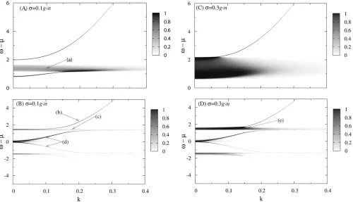
共22兲 The polariton dispersion共22兲from localized excitons has the same structure as from propagating excitons, since the pho-ton dispersion dominates. The spectra, both condensed and uncondensed, are shown in Fig. 1. For a model of dispersive, Bosonic excitons, the equivalent of Eq. 共22兲 has a similar form, but with 2˜⑀→2˜⑀+k2/ 2mex. Over the momentum range

in Fig. 1, the exciton dispersion would lead to a shift of exciton energy of the order of 10−3_g

冑

_{n, i.e., negligible over} the entire scale of Fig. 1. [image:5.612.316.559.57.390.2]

The difference between condensed and uncondensed spectra is dramatic: two new poles appear. These arise be-cause the off diagonal terms in Eq.共12兲mix photon creation and annihilation operators. Such a spectrum may be observed in polariton condensation experimentally, as one may probe the response to inserting a real photon, and observing its emission at a later time. In the presence of a condensate, the polariton is not a quasiparticle. Creating a photon corre-sponds to a superposition of creating and destroying quasi-particles. At nonzero temperature, a population of quasipar-ticles exists, so processes where a quasiparticle is destroyed is possible. This means that a process in which a photon, with energy less than the chemical potential, is added to the system is possible关i.e.,Pabsorbas defined in Eq.共A7兲兴. How-ever, if the system is experimentally probed with photons of energy less than the chemical potential, what will be ob-served is gain, since the absorption of photons is more than

FIG. 1. 共Color online兲 Excitation spectra in the condensed

共grey兲 and uncondensed states, superimposed on the mean-field phase diagram, to show choice of density and temperature. Panel A is for the photon and exciton resonant, and the two spectra are for

T= 2g冑nand␮/g冑n= −1.4 and −0.24. Panel B has the exciton de-tuned by 3g冑n below the photon, and the spectra are for T

= 0.1g冑nand␮/g冑n= −3.29, −3.01, −2.54, and −0.37. The photon mass is m*_{= 0.01. Temperatures and energies plotted in units of}

canceled by spontaneous and stimulated emission.

At small momentum,␰₁corresponds to phase fluctuations of the condensate, i.e., it is the Goldstone mode, and has the form␰1= ±បck, with

c=

冑

1 2m

冉

4ប␻˜₀g2n

␰2共0兲2

冊

冉

兩␺0兩2

N

冊

⬇

冑

␭

2m

␳0

n . 共23兲

The second expression is, for comparison, the form of the Bogoliubov mode in a dilute Bose gas, of interaction strength␭. As␺₀increases, the phase velocity first increases, then decreases. The decrease is due to the saturation of the effective exciton-photon interaction.

The leading-order corrections␰1= ±ck+␣k2are of interest for considering Beliaev decay of phonons.35_{. If␣⬍0,} kine-matic constraints prevent the decay of phonons. For the Bo-goliubov spectrum in a dilute Bose gas,␣= 0, and the cubic term becomes relevant. Here, both signs are possible, accord-ing to whether the spectrum crosses over to the quadratic lower polariton dispersion before this crosses over to a flat exciton dispersion. In most cases,␣⬎0 and ␰₁ will have a point of inflection, but if the exciton is detuned below the photon, then for certain densities,␣⬍0, and the curvature is always negative.

The modes may also be compared to the Cooperon modes in BCS theory. At small momenta, although the mode ␰₁ becomes a pure phase fluctuation, the other mode␰2is not an amplitude fluctuation. To see why this is so, it is helpful to rewrite the action in Eq.共12兲in terms of the Fourier compo-nents of the transverse and longitudinal fluctuations of the photon field. These components, at quadratic order, are equivalent to the phase and amplitude components, and are given by

␦␺␻,k=␺L共␻,k兲+i␺T共␻,k兲,

␦␺¯

␻,k=␺L共−␻,−k兲−i␺T共−␻,−k兲. 共24兲

In terms of these new variables, the action may be written

S=S关␺0兴+␤

兺

i_␻,k

„␺L共−␻,−k兲␺T共−␻,−k兲…

⫻

冉

ប␻˜k+ Re共K1兲+K2 −␻− Im共K1兲

␻+ Im共K₁兲 ប␻˜k+ Re共K1兲−K2

冊

冉

␺L共␻,k兲

␺T共␻,k兲

冊

.

共25兲 Due to the off-diagonal components, the eigenstates are mixed amplitude and phase modes. This mixing vanishes only where␻ is small, which means that the lowest energy parts of the Goldstone mode are purely phase fluctuations. Since the amplitude mode atk= 0 has a nonzero frequency, it will mix with the phase mode.

The off diagonal terms come from two sources. The dy-namic photon field leads to the term ␻. The fermion medi-ated term Im共K₁兲will be nonzero if the density of states is asymmetric about the chemical potential. For the Dicke model, both terms contribute to mixing since

Im共K1兲=g2n

tanh共␤E兲

E

冉

⑀

˜␻

␻2_{+ 4E}2

冊

. 共26兲 Unless˜⑀= 0, the density of states is not symmetric about the chemical potential, and so this term is nonzero.

For BCS superconductivity the pairing field is not dy-namic, so there is no off-diagonal ␻ term. However, there can still be mixing due to Im共K₁兲, which is given by

Im共K1兲=

兺

i_␯,q

␯共⑀q−⑀q+Q兲+␻⑀q

共␯2_+⑀

q

2+⌬2兲关共␯+␻兲2+⑀

q+Q

2 _+⌬2_兴, 共27兲

in which␯ is a Fermionic Matsubara frequency,共2n+ 1兲␲T, and⌬the superconducting gap. Note that this coupling now depends on the momentum transferQas well as energy␻. If the density of states is symmetric, e.g., ⑀q=vFq, then at Q

= 0, Im共K₁兲will be zero, and as the boson field has no dy-namics, the modes will then entirely decouple. In real super-conductors, symmetry of the density of states about the chemical potential is only approximate, and so some degree of mixing will occur.

F. Luminescence spectrum

Although four poles exist, they may have very different spectral weights. At high momentum, the weights of all poles except the highest vanish, and the remaining pole follows the bare photon dispersion.

Such effects can be seen more clearly by plotting the in-coherent luminescence spectrum. As discussed in the Appen-dix, this can be found from the Green’s function as

Pemit共x兲= 2nB共x兲Im关G00共i␻=x+i␩兲兴. 共28兲 It is easier to observe how the spectral weight associated with poles changes after adding inhomogeneous broadening. Figure 2 plots the luminescence spectrum for the same pa-rameters as in Fig. 1, but with inhomogeneous broadening. This will broaden the poles, except for the Goldstone mode 关labeled共d兲in Fig. 2兴, as discussed above. The distribution of energies used is, for numerical efficiency, a cubic approxi-mation to a Gaussian, with standard deviations 0.1g

冑

n and 0.3g

冑

n. The results with a Gaussian density of states have been compared to this cubic approximation, and no signifi-cant differences occur.

transition temperature is adequately described by a model of structureless polaritons.

It is also interesting to consider the uncondensed cases. In Fig. 2共A兲, with the smaller broadening, three lines are vis-ible; the upper and lower polariton, and between them lumi-nescence from excitons weakly coupled to light关labeled共a兲兴. These weakly coupled states arise from excitons further away from resonance with the photon band. Although there may be a large density of such states, they make a much smaller contribution to luminescence than the polariton states, because of their small photon component. With larger broadening, these weakly coupled excitons form a con-tinuum stretching between the two modes, as shown in Fig. 2共C兲.

G. Momentum distribution of photons

From the Green’s function for photon fluctuations, one can calculate the momentum distribution of photons in the cavity. For a two-dimensional cavity coupled via the mirrors to three-dimensional photons outside, the momentum distri-bution may be observed experimentally from the angular distribution.3

When uncondensed,N共p兲is given by

N共p兲= lim

␦→0+具␺p

†_共␶

+␦兲␺p共␶兲典

= lim

␦→0+

␤

冖

dz

2␲inB共z兲e ␦z_G

11共iz,p兲. 共29兲

However, when condensed, since the system is two di-mensional, it is necessary to treat fluctuations more carefully. Writing ␺共r兲=

冑

␳0+␲共r兲ei␾共r兲, the action involves only de-rivatives of the phase, showing that large phase fluctuations are possible. For quadratic fluctuations, one can use the ma-trix in Eq.共25兲describing transverse and longitudinal modes, and relate these to the phase and amplitude excitations.

At low enough temperatures, it is possible to calculate

N共p兲by considering only the phase mode.36_{Thus neglecting} amplitude fluctuations gives

N共p兲= 1

A

冕

d

2_r

冕

_d2_r

⬘

_eik·共r−r⬘兲_␳

0具ei关␾共r兲−␾共r⬘兲兴典 =␳₀1

A

冕

d

2_R

冕

_d2_teik·t_e−D共R+t/2,R−t/2兲_{, 共30兲} where ␳0 is taken as the mean-field photon density. The phase correlator, found by inverting the amplitude-phase ac-tion, is

D共r,r

⬘

兲=

冕

d 2_k

共2␲兲2兵1 − cos关k·共r−r

⬘

兲兴其

m

␤␳0ប2k2

⬇ m

2␲␤␳0ប2

ln

冉

兩r−r

⬘

兩

␰T

冊

. 共31兲

The thermal length is␰T=␤c, where cis the velocity of the

[image:7.612.56.556.62.349.2]

sound mode from Eq.共23兲. This comes from the energy scale

at which fluctuations become cut by the thermal distribution. In this approximation, Eq. 共30兲 may be evaluated exactly37giving

N共p兲= 2␲␳0 共p␰T兲␩

p2

冕

0

⬁

x1−␩J0共x兲dx

= 2␲␳0

␰T␩ p2−␩2

1−␩⌫共1 −␩/2兲

⌫共␩/2兲 , 共32兲

where␩=m/ 2␲␤␳0ប2controls the power-law decay of cor-relations. The second line follows from an identity共see Ref. 38, exercise XVII.32兲. This is valid only for small ␩, far from the transition. The Kosterlitz-Thouless transition39 oc-curs when␩ becomes large, an approximate estimate of the transition is at␩= 2.

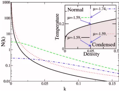
The momentum distribution can therefore be calculated both at low temperatures, where such a scheme holds, and at high temperatures, when uncondensed. This is shown in Fig. 3. When condensed, the power-law divergence leads to a peak normal to the plane. This peak reflects coherence be-tween distant parts of the system, so in a finite system this peak is cut at small momenta.36

IV. FLUCTUATION CORRECTION TO THE MEAN-FIELD THEORY

In this section, we calculate the fluctuation corrections to the mean-field density, and thus to the mean-field phase boundary. Our method is similar to that of Nozières and Schmitt-Rink,40 _{who studied fluctuation corrections to the} BCS mean-field theory for a model of interacting, propagat-ing fermions. However, because our model differs from that of Nozières and Schmitt-Rink, our approach to including second-order fluctuations will also differ. We begin by pre-senting a brief summary of the method used by Nozières and Schmitt-Rink, and further developed by Randeria.33_{We then}

discuss how our approach differs from their work. 1. Fluctuation corrections in three dimensions

To consider fluctuation corrections to a mean-field theory, one first needs to find the partition function in terms of a coherent-state path integral for a Bosonic field,

Z=

冕

D␺exp共−S关␺兴兲.

For the Dicke model,S关␺兴is given in Eq.共5兲. In the work of Nozières and Schmitt-Rink,S关␺兴resulted from decoupling a four-fermion interaction, and then integrating over the fermi-ons. This effective action may be understood as a Ginzburg-Landau theory, with coefficients that are functions of tem-perature and chemical potential as well as the parameters in the Hamiltonian. To find the mean-field phase boundary, one needs both to find the values of temperature and chemical potential where the transition occurs, and to calculate the density evaluated at these parameters.

For the mean-field theory, the action is evaluated for a static uniform field,␺₀, and minimized with respect to this field. At the critical temperature, a second-order phase tran-sition occurs, and the minimum action moves to a nonzero

␺0. The density is found by differentiating the free energy with respect to chemical potential. For the mean-field theory, the free energy is approximated by the action evaluated at

␺0.

To go beyond the mean-field theory, one can expand the effective action about the saddle point:

Z⬇e−S关␺0兴

冕

D␦␺_exp

冉

₋1

2

冏

⳵2_S

⳵␺2

冏

␺0

共␦␺兲2

冊

_{. 共33兲}

This gives an improved estimate of the free energy, from which follows an improved estimate of the density, and thus of the phase boundary. In three dimensions共but not in two, as discussed below兲, one only needs an estimate of the den-sity at the mean-field critical temperature. It is therefore suf-ficient to consider an expansion about the normal-state saddle point, ␺= 0. Such fluctuations may be understood as the contribution to the density from noncondensed pairs of particles, whereas the mean-field estimate of density cluded only unpaired fermions. These corrections will in-crease the density at a fixed critical temperature, or equiva-lently decrease the critical temperature for a given density.

Because of features of our model, our approach differs from that of Nozières and Schmitt-Rink; two differences in our model are of particular importance. First, our boson field is dynamic, and there exists a chemical potential for bosons. In this respect, our model is closer to the boson-fermion models25,26 _{studied in the context of Feshbach resonances,} for which Ohashi and Griffin27 _{have studied fluctuation} cor-rections. Second, we consider a two-dimensional system; this requires calculation of fluctuations in the presence of a con-densate, as discussed in the next section.

2. Fluctuations in two dimensions

To find the fluctuation correction to the mean-field phase boundary in two dimensions, it is necessary to consider

fluc-FIG. 3.共Color online兲Momentum distribution of photons, from which follows the angular distribution. These are plotted for low-temperature condensed systems, where the approximation of includ-ing only phase fluctuations is valid, and for the simpler, uncon-densed case. The inset illustrates the choices of density and temperature.共Parameters are⌬*_{= 1,m}*_{= 0.01, wave vector plotted}

[image:8.612.76.270.56.205.2]

tuations in the presence of a condensate. Considering fluc-tuations in the normal state would lead to the conclusion that the normal state can support any density: As one approaches the mean-field critical temperature, the fluctuation density will become infrared divergent, allowing any density. This correctly indicates that no long-range order exists in two di-mensions; however, a Kosterlitz-Thouless39,41_{transition does} occur.

Instead one must start by considering fluctuations in the presence of a condensate. This gives a density, defined by the total derivative of free energy with respect to chemical po-tential, of the form

␳= −dF

d␮= −

⳵F

⳵␮−

⳵F

⳵␺0

d␺0

d␮. 共34兲

When considering fluctuation corrections in the presence of a condensate, in any dimension, one must take care to consider the depletion of the order parameter due to the in-teraction between condensed and uncondensed particles. This is discussed in detail in Sec. IV A. Such a depletion means that, for a fixed temperature, the critical value of the chemical potential changes; at the mean-field critical chemi-cal potential the formula for total density may become nega-tive. It is therefore necessary to make a separate estimate of the order parameter in the presence of fluctuations, and de-fine the phase boundary where the order parameter goes to zero.

In three dimensions such a calculation can be achieved by identifying parts of the density as the population of the ground state and of fluctuations共as discussed below in Sec. IV A 2b兲. In two dimensions, no true condensate exists, but a quasicondensate with a cutoffk0 can be considered. As dis-cussed by Popov,42_{the quasicondensate and fluctuation} den-sities both contain terms which diverge logarithmically as

k0→0, but these divergences cancel in the total density. Instead, in two dimensions, one must consider an alternate definition for the location of the phase boundary. Since the transition is a Kosterlitz-Thouless transition, one should map the problem to the two-dimensional Coulomb gas.43_This re-quires the vortex core energy and strength of vortex-vortex interactions, which both scale asប2_␳

s/ 2m, where␳sis a

su-perfluid response density. The phase transition thus occurs when␳s= # 2mT/ប2. The numerical prefactor depends on the

vortex core structure. However, approximating the critical condition by␳s= 0 leads to only a small shift to TC.

A. Total derivatives and negative densities

This section discusses the effects and interpretation of the second term in Eq.共34兲. In Eq.共3.41兲of Ref. 27, Ohashi and Griffin define the density as the partial derivative of free energy with respect to chemical potential, neglecting the sec-ond term in Eq.共34兲, which they describe as a higher-order correction under the Gaussian fluctuation approximation. As shown below in Sec. IV A 1, the contribution of the second term in Eq. 共34兲 to the density should not necessarily be neglected in the Gaussian fluctuation approximation. Section IV A 2 shows explicitly that the two terms in Eq.共34兲are of the same order. The existence of the second term is crucial in

finding a finite density in two dimensions, however, may be less important in three dimensions.

1. Gaussian fluctuation approximation

In Sec. IV A 2 we will show that the second term in Eq. 共34兲is of the same order as the first. Before this, we explain why the second term of Eq.共34兲should not be automatically neglected. Even though it is of the form⳵3S/⳵␺₀3, such terms are not necessarily small, and can contribute to the density at quadratic order.

To see that a Gaussian theory may be correct even if such third-order terms are not small, consider an expansion of the effective action,

S=S关␺0兴+

d2S d␺₀2␦␺

2₊ d 3_S

d␺₀3␦␺

3_{+ ¯. 共35兲}

A Gaussian approximation is justified if, using this action, the expectation of the cubic term is less than the quadratic term. This condition can be written as

冉

d2S d␺₀2

冊

3/2

Ⰷ d3S

d␺₀3. 共36兲

This need not require that the coefficient of the cubic term is smaller, i.e., that

d2S d␺₀2Ⰷ

d3S d␺₀3.

In fact, if both terms are of the same order, but large;

d2S/d␺₀2⯝d3S/d␺₀3Ⰷ1, then the condition共36兲is fulfilled. Writing the free energy including fluctuations schemati-cally as

F=S关␺0兴+ ln

冋

冕

D␦␺exp

冉

−

d2S d␺₀2␦␺

2

冊

册

_{, 共37兲}

the fluctuation contribution to the second term in Eq. 共34兲 will take the form

␳= ¯ +

冓

d 3_S

d␺₀3␦␺

2

冔

d␺0

d␮, 共38兲

where 具¯典 signifies averaging over the fluctuation action. Thus in calculating the condensate density, there is a term which depends on ⳵3_S/⳵␺

0

3 _{but only involves second-order} expectations of the fields. Since ⳵3_S/⳵␺

0

3 _{is not necessarily} small, and it contributes to the density at quadratic order, there is noa prioriargument for neglecting this term. In the following we show explicitly that this term should be in-cluded.

2. Total derivatives for a dilute Bose gas

H−␮N=

兺

k

共⑀k−␮兲ak†ak+ g

2_k

兺

,k⬘,q

ak†+qak⬘−q

†

akak⬘. 共39兲

Further, the terms in Eq.共34兲will be interpreted by consid-ering the Hugenholtz-Pines relation at one loop order, as dis-cussed in Ref. 42.

Saddle point and fluctuationsTo find the free energy, con-sider the static uniform saddle point,具a₀†a0典=兩A兩2=␮/g, and quadratic fluctuations, which are governed by the Hamil-tonian

H_eff=

兺

k

共⑀k−␮+ 2gA2兲ak†ak+ gA2

2 共ak †_a

−k

† _+a

ka−k兲.

共40兲

Thus by a Bogoliubov transform, the free energy and density become

F= −␮A2+g 2A

4₊

兺

k

冉

1

␤ ln共1 −e−␤Ek兲+

1

2共Ek−⑀k−␮兲

冊

, 共41兲

␳=A2−

兺

k

冉

nB共Ek兲

⑀k Ek

+⑀k−Ek 2Ek

冊

, 共42兲

whereEk=

冑

⑀k共⑀k+ 2␮兲.

The total density is thus less than the saddle pointA2, and could be negative. From the form of the fluctuation Hamil-tonian, Eq.共40兲, usinggA2=␮, it can be seen that the fluc-tuation contribution is

␳f= −

兺

k

再

具ak

†

ak典+

1 2共具ak

†

a₋k

† _典

+具aka−k典兲

冎

. 共43兲

Using the results

具ak†ak典=nB共Ek兲

⑀k+␮ Ek

+⑀k+␮−Ek 2Ek

, 共44兲

具ak

†

a₋k

† _典

=具aka−k典= −

␮

Ek

冉

nB共Ek兲+

1

2

冊

, 共45兲 it is clear this matches Eq.共42兲.

In contrast, taking partial derivatives, and neglecting the second term in Eq. 共34兲 gives␳f=兺k具ak

†_a

k典. In two

dimen-sions, for ␮⫽0, this expression will be infrared divergent, while Eq.共42兲is not.

Hugenholtz-Pines relationTo identify the meaning of the terms in Eq. 共43兲, one can consider the Hugenholtz-Pines relation for the normal and anomalous self-energiesA共␻,k兲,

B共␻,k兲, respectively:

A共0,0兲−B共0,0兲=␮. 共46兲 The approximations in the previous section are equivalent to evaluating A and B at one-loop order. As explained by Popov,42_{this becomes}

␮= 2g共␳0+␳1兲−g共␳0+␳˜1兲− 2g2␳0

兺

k

关G共k兲G共−k兲

−G₁共k兲G₁共−k兲兴. 共47兲

Here ␳₀ is the new condensate density, ␳₁ the density of noncondensed particles, and˜␳₁is an anomalous particle den-sity, ␳˜₁=兺kG1共k兲, with G1 the anomalous Green’s function. The last term is a second-order correction due to the three boson vertices of the formgA共a†_a†_a+a†_{aa兲. This last term in} Eq.共47兲can be evaluated to be 2g␳˜₁, leading to the result

␳0=

␮

g −共2␳1+␳˜1兲, 共48兲

showing that␳0+␳1 is less than the saddle-point density. Compare this expression for the total density to that from saddle point and fluctuations,

␳=␳0+␳1=␳s.p.−

⳵Ffluct

⳵␮ −

d␺0

d␮

⳵Ffluct

⳵␺0

, 共49兲

where␳s.p.=␮/g is the saddle-point expectation of the den-sity, andFfluctis the free energy from the fluctuation contri-butions. Since␳1, the density of noncondensed particles can be identified as

␳1=

兺

k

具ak†ak典= −

⳵F_fluct

⳵␮ , 共50兲

one must identify the depleted condensate density, Eq.共48兲 with

␳0=

␮

g − d␺0

d␮

⳵Ffluct

⳵␺0

. 共51兲

The derivatives with respect to the order parameter there-fore describe a depletion of the order parameter due to fluc-tuations. Physically, interactions between the condensate and the finite population of noncondensed particles共at finite tem-perature兲push up the chemical potential. With such a theory, there now exists a region of parameter space which is not condensed, but␮⬎0. In such a region it is essential to in-clude modifications of the particle spectrum due to interac-tions to describe the normal state.

Comparison of methods The phase boundary for the WIDBG model with static interactions is peculiarly insensi-tive to the calculation scheme. This can be seen by consid-ering the Hugenholtz-Pines relation at the transition. In gen-eral, the anomalous self-energy vanishes at the transition, so

␮=A共0 , 0兲. Since␳0= 0, the total density is␳1, which may be found from the fluctuation Green’s function,␳=兺_␻,kG共␻,k兲,

G共␻,k兲=关i␻+⑀k−A共0,0兲+A共␻,k兲兴−1, 共52兲

where␮=A共0 , 0兲 has been used. If the self-energy is static,

A共␻,k兲=A共0 , 0兲, then at the transition the quasiparticles are exactly free. Any approximation scheme which gives

remain true for dynamic self-energies.

For a boson-fermion model, such as polaritons, because of the dynamic self-energy, total and partial derivatives will give different answers. For the three-dimensional case stud-ied by Ohashi and Griffin, this will lead to critical tempera-tures differing by a numerical factor, but in two dimensions using partial derivatives gives divergent answers. Were one to use partial derivatives, the density calculated from the condensed and noncondensed phases would agree at the critical chemical potential. However, for the total derivative, the density calculated at the new critical potential need not agree with that calculated from the noncondensed phase. A difference between these results reflects the fact that both are approximations of the phase boundary, and is indicative of the Ginzburg criterion.

B. Total density for condensed polaritons

From the effective action, Eq. 共12兲, the free energy per unit area, including quadratic fluctuations may be written as

F A=

S关␺0兴

A +

1

␤

冕

0

⬁ _d2_k 共2␲兲2

兺

␻ ln关兩i␻+ប␻k+K1共␻兲兩

2

−兩K2共␻兲兩2兴=

再

ប␻˜k

兩␺0兩2

A −

␮n

2 −

n

␤ln关cosh共␤E兲兴

冎

+

再

1

␤

冕

0

⬁ _d2_k

共2␲兲2ln关1 −e

−␤ប␻˜_k兴

冎

_共

53兲

+ 1

␤

冕

0

K_m d2_k 共2␲兲2

再

ln

冋

sinh共␤␰₁/2兲sinh共␤␰₂/2兲 sinh共␤E兲sinh共␤ប␻˜k/2兲

册

+1 2ln

冋

1 −

␣4E2

2共ប␻˜kE2−ប␻˜0˜⑀2兲

册

冎

. 共54兲

Here E, ␣, and ␰1,2 are defined as in Sec. III. The first term in braces isS关␺0兴, the second and third together are the fluctuation corrections. As discussed in Sec. II A, the inter-action has been cut off at a scale Km, so for k⬎Km, the action is that of a free gas of photons, i.e., the second term in braces. In the third term, there are contributions both due to the Matsubara sum of Eq.共17兲, and due to the ␦_␻ terms in Eq.共12兲, as discussed further in the Appendix, Sec. II.

The total density is then given by

␳=兩␺0兩 2

A +

n

2

冋

1 −

⑀

˜

Etanh共␤E兲

册

+

冕

₀ K_m

d2_k

共2␲兲2

再

f关␰1兴+f关␰2兴

−f关2E兴+1

2 +g共k兲

冎

+

冕

K_m

⬁ _d2_k

共2␲兲2nB共ប␻˜k兲, 共55兲

where

f关x兴=

冉

nB共x兲+ 1 2

冊冉

−

dx d␮

冊

, g共k兲= − 1

2␤ 1 共1 −C兲

dC d␮,

C= ␤sech

2_共␤E兲g2_n 2共ប␻˜kE2−ប␻˜0˜⑀2兲

g2兩␺0兩2

A .

In going from Eq. 共54兲 and 共55兲 the two integrals have been re-arranged, the second now describing only the free, high-energy photons. Again, the last term,g共k兲, arises due to the␦_␻terms.

The derivatives of polariton energies that arise in calcu-lating the density may be given in terms of the expressions

A共k兲,B共k兲as defined in Eq. 共18兲: 2␰_1,2

d␮ =

1 4␰1,2

冋

dA共k兲 d␮ ±

1

冑

A共k兲2−B共k兲

⫻

冉

2A共k兲dA共k兲 d␮ −

dB共k兲

d␮

冊

册

, 共56兲

dA共k兲 d␮ = 8E

dE

d␮− 2ប␻k− 4˜⑀− 2ប␻˜0, 共57兲

dB共k兲 d␮ = 16

ប2_k2 2m

冉

2E

dE d␮ប␻˜k−E

2_{+˜⑀ប␻˜}

0+˜⑀2

冊

. 共58兲 To find dE/d␮ in the presence of a condensate, one can differentiate the gap equation, Eq.共6兲, giving

− 1 =dE

d␮ g2n

2E2关␤Esech

2_{共␤E兲− tanh共␤E兲兴. 共59兲}

C. Two dimensions, superfluid response

Having found an expression for the total density including fluctuations, it is necessary to consider how fluctuations change the critical chemical potential. As discussed in the introduction to this section, in two dimensions this requires consideration of the Kosterlitz-Thouless phase transition. The phase boundary is approximated from the condensed state by the chemical potential at which the superfluid re-sponse vanishes. We therefore must calculate the normal and superfluid response in the presence of a condensate.

1. Calculating normal response density

Following the standard procedure,44,45 _{we consider the} current,

J共q,0兲=

兺

k,␻

បk

m␺k−q/2

† _␺

k+q/2. 共60兲

For a perturbation ␦H=ប␦l·J, the linear response may be written 具Ji共q, 0兲典=␹ij共q兲␦lj共q兲. By symmetry, the most

gen-eral response function is

␹ij共q兲=␹L共q兲

qiqj

q2 +␹T共q兲

冉

␦ij− qiqj

q2

冊

. 共61兲

By gauge symmetry, Eq.共60兲is a conserved current. It fol-lows, via a Ward identity, that qi␹ij共q兲=qjTr关G共k兲兴, so the

response depends on only the density of normal particles,

␳normal=m␹T共q→0兲/A.

In order to calculate the total density correctly, it is nec-essary to introduce vertex corrections, i.e.,

␹ij共q→0兲= Tr„⌫i共k,k兲G共k兲␥j共k,k兲G共k兲…, 共62兲

where␥i共p,q兲=␴3共pi+qi兲/ 2m, and⌫i共p,q兲is chosen to

sat-isfy the Ward identity. However, the diagrams required to satisfy the Ward identity共see Ref. 44兲take the form

⌫i共p,q兲=␥i共p,q兲+共pi−qi兲f共p,q兲. 共63兲

This form of the vertex correction means only the longitudi-nal response is affected. Therefore the standard procedure is to calculate the total density directly from the free energy, as

in Sec. IV B, and the normal density by linear response. To one-loop order, and neglecting vertex corrections, the response function is given by

␹ij共q→0兲=

1

␤

兺

k,␻

ប2_k

ikj

m2 Tr关G共k兲␴3G共k兲␴3兴, 共64兲

and so, taking the continuum limit, the normal density is given by

␳n=

冕

0

⬁ _d2_k 共2␲兲2

ប2_k2 2m

1

␤

兺

␻

Tr关G共k兲␴₃G共k兲␴₃兴. 共65兲 For the polariton system, the trace can be evaluated to give

␳n=

冕

0

⬁ _d2_k 共2␲兲2

ប2_k2 2m

1

␤

兺

␻

关i␻+ប␻˜k+K1共␻兲兴2+关−i␻+ប␻˜k+K1

*_共␻兲兴2_{− 2兩K} 2共␻兲兩2 关兩i␻+ប␻˜k+K1共␻兲兩2−兩K2共␻兲兩2兴2

共66兲

=

冕

0

⬁ _d2_k 共2␲兲2

ប2_k2 2m

1

␤

再

兺

_␻

关2␻˜₀共i˜⑀␻−E2−˜⑀2_{兲+共i␻+␻˜}

k兲共␻2+ 4E2兲兴2−关2␻˜0共E2−˜⑀2兲兴2 共␻2_+␰

1

2_兲2_共␻2_+␰ 2

2_兲2 + C0共k兲

冎

. 共67兲

Again, in evaluating the Matsubara sum, one must consider the␦_␻ terms. The termC0共k兲is the difference between the true term at␻= 0, and the analytic continuation appearing in the Matsubara sum in Eq.共67兲, and is given by

C0共k兲= 2␣⫻

冋

冉

ប2_k2 2m

冊

冉

ប2_k2 2m +

g2_兩␺ 0兩2

A ប␻˜₀

E2

冊冉

ប2_k2

2m + g2_兩␺

0兩2

A ប␻˜₀

E2 − 2␣

冊

册

−1

, 共68兲

with␣ as defined in Eq.共15兲.

2. Total photon density

For the polariton system there is an added complication. Equation共67兲 gives the density of normal photons, but Eq. 共55兲is the total excitation density共including excitons兲. It is therefore necessary to calculate the total photon density.

This can be done by considering separate chemical poten-tials for photons and excitons, which are set equal at the end of the calculation. This means making the change,

␮N→␮ex.

兺

j=1

j=nA

冉

Sj z

+1

2

冊

+␮phot.

兺

k

␺k

†_␺

k, 共69兲

in the action. The photon density is then total derivative with respect to the photon chemical potential␮phot.

This density is given by Eq.共55兲with two changes. First, the mean-field exciton density,

n

2

冋

1 −

⑀

˜

Etanh共␤E兲

册

, 共70兲

should be removed. Second, in f关x兴,g共k兲 derivatives should be taken with respect to ␮phot. This means replacing Eqs. 共57兲and共58兲by

dA共k兲 d␮phot.

= 8EdE

d␮− 2ប␻k− 4˜⑀, 共71兲

dB共k兲 d␮_phot.= 16

ប2_k2 2m

冉

2E

dE d␮␻˜k−E

2_+˜⑀2

冊

_{. 共72兲} This makes use of the fact thatdE/d␮phot=dE/d␮, as can be seen from the gap equation.

V. PHASE BOUNDARY INCLUDING FLUCTUATIONS

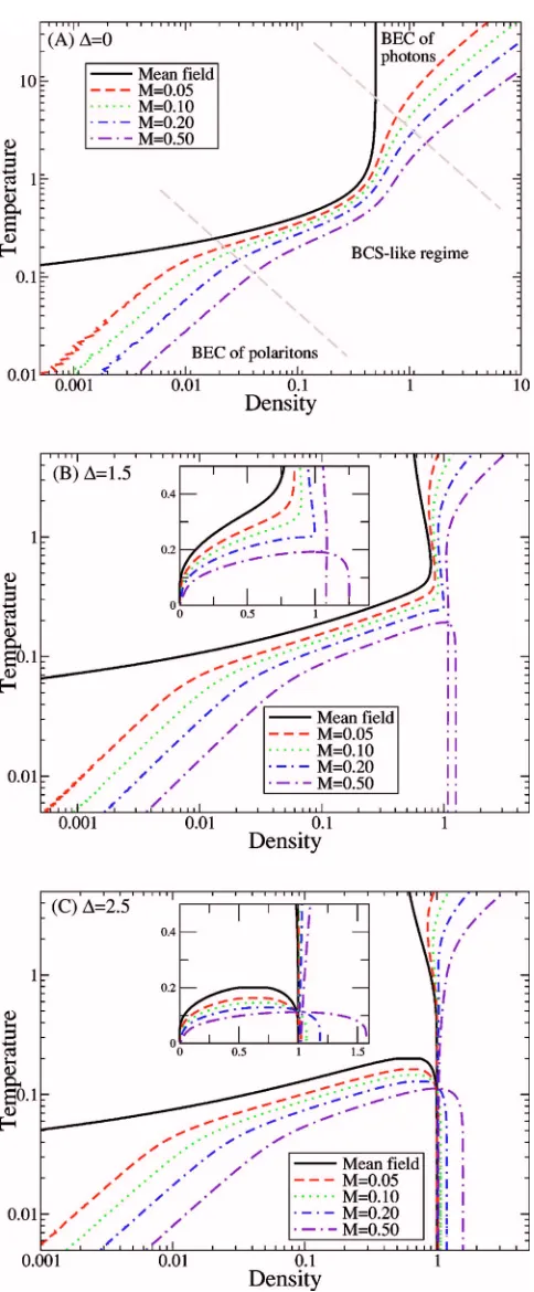
Combining the results of Sec. IV, the phase boundary is found by plotting the total density关Eq.共55兲兴at the value of chemical potential where the normal photon density 关Eq. 共67兲兴 matches the total photon density 共discussed in Sec. IV C 2兲. The phase boundaries found in this way are plotted in Fig. 4. The form of the phase boundary can be explained by considering how, at finite temperatures, the occupation of excited states of the system depletes the condensate. Which excited states are relevant changes with density.

A. Resonant case

shal-low slope, and consequently a large density of states. Such excitations are described in a model of point bosons. The phase boundary can therefore be estimated from the degen-eracy temperature of a gas of polaritons, of mass 2m, where

mis the bare photon mass:

k_BTdeg=

2␲ប2 2共2m兲␳=g

冑

n

␲

2m*

␳

n. 共73兲

As the density increases, the phase mode becomes steeper, and so has a smaller density of states. The relevant excita-tions are then single-particle excitaexcita-tions across the gap. Such excitations are accounted for in the mean-field theory. Com-bining Eqs.共6兲and共7兲gives the result

k_BTc=g

冑

n

冑

1 − 2␳/n

2 tanh−1共1 − 2␳/n兲⬇ g

冑

n

− ln共␳/n兲. 共74兲

As seen in Fig. 4, the mean-field boundary is effectively constant on the scale of the boundary for BEC of point bosons, and so the crossover to mean field always occurs nearkBT⬇g

冑

n, the Rabi splitting. The density at which this crossover occurs depends on the photon mass. Comparing Eqs. 共73兲 and 共74兲, this crossover occurs at a density

␳crossover⬇nm*.

In terms of the measurable Rabi splitting,g

冑

n, and polar-iton massm, this gives the density

␳crossover=

mg

冑

n

ប2 . 共75兲

For the structures studied by Yamamoto et al.,2–4 _g

冑

_n ⬇7 meV and m⬇10−5_m

electron. These values give a cross-over density of␳crossover= 2.6⫻108cm−2. This is both much less than the estimates of experimentally achieved density,

n⬃1011cm−2 per pulse, and also much less than the Mott density in this structure, nMott⬇3.6⫻1013cm−2. For the structures studied by Dang et al.,1,5 _g

冑

_{n⬇13 meV, and m} ⬇3⫻10−5melectron, so crossover densities are again of the same order,␳crossover= 5⫻108cm−2. Danget al. also present results for the detuned case,5_{discussed below, with a range} of dimensionless detunings 0.5⬎⌬*_⬎−0.7.

Equation共75兲describes the crossover in terms of proper-ties measurable for a given microcavity. However, to under-stand what fundamental length scales control this crossover density, it is necessary to write the coupling strength and polariton mass in terms of the dimensions of the cavity and properties of the excitons. Using the expressions in Sec. II for photon mass and coupling strengthg, this gives the cross-over density as

␳crossover= 4␲2

冑

e2 4␲␧0បc

1

␧r1/4

dab冑n

w2 . 共76兲

The crossover density is therefore controlled by two pa-rameters: The width of the cavitywand the ratio of electron-hole separation to average two-level system separation,

dab

冑

n=dab/rseparation. If the average two-level system separa-tion共rseparation兲is less than the electron-hole separation共dab兲,

then our model of localized two-level systems will break down. Therefore within our model the largest possible

cross-FIG. 4. 共Color online兲 Mean-field phase boundary, and phase boundaries including fluctuation correction for four values of pho-ton mass, on a logarithmic scale共Insets are on a linear scale兲. Panel

[image:13.612.54.296.48.633.2]

over density scale is 1 /w2_{. This length scale occurs because} the cavity size controls the wavelength of the lowest radia-tion mode. Crossover to a BCS-like mean-field regime oc-curs when the density approaches a scale set by the wave-length of light, rather than one set by the exciton Bohr radius. Therefore in general this crossover density is much less than the Mott density.

At yet higher densities, the single-particle excitations are saturated, and so the condensate becomes photon dominated. In this regime, the transition temperature is that for a gas of massive photons. If the photon mass is large 共m*_{⬎1兲, a} mean-field regime never exists, instead the phase boundary changes directly from polariton condensation to a photon condensation. However, since for experimental parameters the dimensionless mass is only of the order of 10−3_{, a} mean-field regime will exist. These various crossovers are illus-trated schematically in Fig. 5.

B. Effects of detuning

If the excitons are detuned below the photon 共positive detuning兲, it becomes possible for the system to reach half filling while remaining uncondensed. For positive detunings greater than 2g

冑

n the mean-field phase boundary becomes re-entrant, as shown in the bottom panel of Fig. 4. For smaller but still positive detunings, the mean-field boundary has a maximum critical density at a finite temperature, but no maximum of critical temperature. The opposite case, of ex-citons detuned above photons, shows no interesting features; the system will always condensed before half filling.

This multivalued phase boundary is discussed in Ref. 14, and can be explained in terms of phase locking of precessing spins,46 _{either about spin-down 共low density兲 or spin-up} 共high density兲states. Above in