Compositional Reasoning for Markov Decision Processes

(Extended Abstract)

Yuxin Deng1and Matthew Hennessy2

1 _{Shanghai Jiao Tong University, China} 2 _{Trinity College Dublin, Ireland}

Abstract. Markov decision processes (MDPs) have long been used to model qualitative aspects of systems in the presence of uncertainty. However, much of the literature on MDPs takes a monolithic approach, by modelling a system as a particular MDP; properties of the system are then inferred by analysis of that particular MDP. In this paper we develop compositional methods for reasoning about the qualitative behaviour of MDPs. We consider a class of labelled MDPs called weighted MDPs from a process algebraic point of view. For these we define a coinductive simulation-based behavioural preorder which is compositional in the sense that it is preserved by structural operators for constructing MDPs from components.

For finitary convergent processes, which are finite-state and finitely branching systems without divergence, we provide two characterisations of the behavioural preorder. The first uses a novel qualitative probabilistic logic, while the second is in terms of a novel form of testing, in which benefits are accrued during the execution of tests.

1

Introduction

Markov decision processes (MDPs) have long been used to model qualitative aspects of systems in the presence of uncertainty [9, 10, 1]. A comprehensive account of analysis techniques may be found in [9], while [10] provides a good account ofmodel-checking.

However much of the literature on MDPs takes a monolithic view of systems; es-sentially a system is modelled using a particular MDP, and properties of the system are then inferred by analysis of that MDP. In this paper, instead, we would like to develop compositional methods for reasoning about qualitative behaviour of Markov decision processes. This involves defining an appropriate method for comparing the behaviour MDPs which is susceptible to compositional analysis; the behaviour of a composite system should be determined by that of its components.

s0

sd

up3

down1

t0

td

up2

down4

u0

τ0

τ1

up1

τ2

down1

up1

The first, a two-state machine, continually performs anupaction, which accrues a ben-efit of 3 units, followed by adownaction, which accrues a benefit of 1. The second ma-chine performs the same actions but with benefits 2 and 4 respectively. In some senset0 is an improvement ons0; intuitivelyt0can simulate the behaviour ofs0but in so doing accrue more benefits; this is true even if one of its actionsupis less beneficial than the corresponding action ofs0. The same is true for the machineu0; it can also simulate the behaviour ofs0, with more benefit, although in this case some internal weighted actions, denoted byτ, participate in the simulation and add to the accumulation of benefits. In our terminology we will writes0 vsimt0, s0 vsimu0.However we will havet06vsimu0 because althoughu0can simulate the behaviour oft0it accumulates less benefit.

Similar informal reasoning can also be applied to probabilistic systems. Consider the following systems:

s1

O T

up₂

1 4

3 4

down3

down1

t1

U

R D

up₂

τ0

3 4

1 4

τ1

down1

The mixture of probabilistic behaviour and internal actions introduces complica-tions. Consider the systemt1above which after performing anupprobabilistically de-cides internally whether to perform adownaction for benefit 1, or branch back to make another probabilistic choice. However each time it reverts back it accumulates a non-zero benefit via the internal weighted action τ1, albeit with diminishing probability. Nevertheless it will turn out that for our definition of simulation s0 vsim t1and indeed s1vsimt1.

Systems exhibiting both probabilistic and nondeterministic behaviour require more complicated analysis. Consider the following system:

s2

S T

up1

1 4

3 4

down2

down1

down6

After performing the actionupit finds itself either in a state in which the actiondown

will accrue the benefit 2, or 25% of the time there will be a nondeterministic choice between it accruing either 1 or 6. In the literature there are numerous mechanisms, such as policies, schedulers, adversaries, etc. [9, 11, 10] for resolving such choices. Here one can see if this choice systematically leads to the lower benefit 1 thens2will not simulate s0as it does not accrue sufficient benefits. This is a pessimistic outlook; an optimistic outlook means that the best choices are systematically made. If this is assumed then we will haves0 vsims2; ins2one execution ofupfollowed bydownwill yield on average the benefit 1+(3₄·2+1₄·6)=4.

The main contribution of the paper is a coinductively defined behavioural preorder vsim between MDPs based on simulations which validate the examples discussed in-formally above. We confine our attention to the optimistic approach to the resolution of nondeterministic choices, although in a later paper we hope to investigate the pes-simistic approach. We also show that this preorder is compositional in the sense that it is preserved by structural operators for constructing MDPs from components. The main operator is one for composing two MDPs in parallel. In P | Qthe two MPDsPand Qremain independent, execute in parallel and may communicate by synchronising on complementary actions; these internal synchronisations accrue the combined benefits of the associated complementary actions.

For finitary convergent MDPs, which are finite-state and finitely branching systems without divergence, we also provide two characterisations for the behavioural preorder v_sim. The first is in terms of aqualitative probabilistic logicL_Q. In addition to the stan-dard logical connectives∧, ∨and both maximal and minimal fixpoints this contains a novel qualitativepossibilitymodalityhαi

w(φ1p⊕φ2), where pis some probability

benefitwby performing the actionα, and subsequently satisfy the probabilistic asser-tion φ1 p⊕ φ2. It turns out that the simulation preorder is completely determined by the logic L_Q. Further evidence of the compatibility between the logic and the simu-lation resimu-lation is the fact that every systemPhas acharacteristic formulaφ(P) in the logic which captures its behaviour; informally systemQcan simulatePif and only if it satisfies the characteristic formulaφ(P).

Our second characterisation is in terms of a novel form of testing calledbenefits testing. Intuitively a systemPcan be tested by running it in parallel with another testing systemT, and seeing the possible accrued benefits. In the presence of nondeterminism the execution of the combined system (T |P) will result in a non-empty set of benefits, Benefits(T |P). Then systemsPandQcan be compared by comparing the associated benefit setsBenefits(T |P) andBenefits(T |Q) whereT ranges over some collection of possible tests. We show that the simulation preordervsimis also determined in this manner by a suitable collection of testsT.

The rest of this paper is organised as follows. In Section 2 we introduce the model of weighted MDPs, the notation of hyper-derivations and some important properties. Then we define a behavioural preorder based on amortised weighted simulations, which turns out to be a precongruence in a CCS-like process calculus for MDPs. Next, we provide logical and testing characterisations of the behavioural preorder over finitary conver-gent processes. In Section 3 we present a qualitative probabilistic logic whose formulae completely determine the behavioural preorder. We also show that characteristic formu-lae can be constructed for any state in such an MDP. In Section 4 we propose a testing framework where our behavioural preorder is sound and complete for may testing pre-order. Finally, we conclude in Section 5.

Due to lack of space, we omit all detailed proofs: they are reported in [3].

2

Simulations for weighted Markov decision processes

There is considerable variation in the literature in the formal definition of a (labelled) Markov decision process [10, 9]. For the purpose of this paper we use Definition 1.

We first fix some notation. A (discrete) probability subdistribution over a set S is a function∆ :S → [0,1] withP

s∈S∆(s) ≤1; the support of such an∆is the setd∆e= {s∈S | ∆(s)>0}. A subdistribution is a (total, or full) distribution ifP

s∈S∆(s)=1. The point distributionsassigns probability 1 tosand 0 to all other elements ofS , so thatdse=s. We useDsub(S) to denote the set of subdistributions overS , andD(S) its subset of full distributions.

Let{∆k|k∈K}be a set of subdistributions, possibly infinite. ThenPk∈K∆kis the real-valued function inS →_Rdefined by (P

k∈K∆k)(s) :=Pk∈K∆k(s). This is a partial operation on subdistributions because for some statesthe sum of∆k(s) might exceed 1. If the index set is finite, say{1..n}, we often write∆1+. . .+∆n. Forpa real number from [0,1] we usep·∆to denote the subdistribution given by (p·∆)(s) := p·∆(s). Finally we useεto denote the everywhere-zero subdistribution that thus has empty support. These operations on subdistributions do not readily adapt themselves to distributions; yet ifP

k∈Kpk=1 for some collection ofpk≥0, and the∆kare distributions, then so is

P

Definition 1 (Weighted Markov decision process).Aweighted Markov decision pro-cessor wMDP is a 4-tuplehS,A,W,−→iwhere S is a set of states,Aa set of actions, W a set of weights, and−→ ⊆ S ×A×W × D(S). We normally write s −→α _w ∆to mean(s, α,w, ∆) ∈−→. In this paper we set W to be_R≥0, the set of non-negative real numbers, and we assumeAhas the structureActτ=Act∪ {τ}where, for the purpose of communication, each a inActhas an inverse a satisfying a=a. ut

A wMDP is

– finite-stateifS is a finite set;

– finitely branchingif for each states, the set{(α,w, ∆)|s−→α _w∆}is finite; – finitaryif it is both finite-state and finitely branching.

In the Introduction we have used a straightforward graphical representation for wMDPs;

a statesis represented by a node s while darkened circular nodes are used for dis-tributions, and arrows between nodes and distributions are annotated with their weights. Often a point distribution is represented by the unique state in its support; see the first series of examples with initial statess0,t0andu0.

2.1 Hyper-derivations

As we have seen in the Introduction, when reasoning informally thatt1 can simulate s0, the limiting behaviour of internal computations must be taken into account. We formalise this by extending the approach originally given in [4].

In a wMDP actions are only performed by states, in that actions are given by rela-tions from states to distriburela-tions. But formally, systems or processes in general corre-spond to distributions over states, so in order to define what it means for a process to perform an action, we need toliftthese relations so that they also apply to distributions. In fact we will find it convenient to lift them to subdistributions.

Definition 2. LetR⊆S ×(_R≥0× Dsub(S))be a relation from states to pairs of weights and subdistributions. ThenR ⊆ Dsub(S)×(R≥0× Dsub(S))is the smallest relation that satisfies:

(i) sR hr, Θiimplies sR hr, Θi, and

(ii) (Linearity)∆i R hri, Θiifor i∈I implies(Pi∈Ipi·∆i) R (Pi∈Ipi· hri, Θii)for any pi∈[0,1](i∈I) withPi∈Ipi≤1. ut

An application of Definition 2 to the arrow relation −→α in a wMDP gives a relation

Definition 3 (Hyper-derivations).A hyper-derivation consists of a collection of sub-distributions∆, ∆→_k , ∆×_k, for k≥0, with the following properties:

∆ = ∆→

0 +∆

×

0

∆→

0 τ −→w0∆

→

1 +∆

× 1 .. . (1) ∆→ k τ

−→_wk ∆→_k+1+∆×_k+1

.. .

∆0 ₌ ∞ X

k=0

∆×

k

Then we call∆0 = P∞

k=0∆

×

k ahyper-derivativeof∆, and write∆ τ

=⇒w ∆0, where w =

P

k≥0wk, to mean that∆can make a(weak) hyper-moveto its derivative∆0with weight w. Note that in general w∈_R≥0∪{∞}; that is there is no guarantee that the sumP

k≥0wk

has a finite limit. ut

Example 1. Consider the wMDP with initial state t1 discussed in the Introduction. Then we have the following hyper-derivation:

U = U+ε

U −→τ 0 3 4 ·R+

1 4·D 3

4·R τ −→3

4 3 4 ·U+ε 3

4 ·U τ −→₀ (3

4) 2_·

R+(3 4)

1 4·D

(3 4)

2_{·R −→}τ (3

4)2 ( 3 4)

2_·U+ε

.. .

(3 4)

k_{·U −→}τ 0 (

3 4)

(k+1)_·R+(3 4)

k1 4·D

(3 4)

(k+1)_·R−→τ (3

4)(k+1) ( 3 4)

(k+1)_·U+ε

.. .

That is,U=⇒τ _wP

k≥0(34) k₍1

4 ·D) wherew=

P

k≥1(34)

k_{. However this weight evaluates}

to 3, while the sum of the sub-distributions is the full point distribution D. In other

wordsU=⇒τ 3 D. ut

Because of the complexity of hyper-derivations the following has a non-trivial proof:

The generation of a hyper-derivative is in general highly nondeterministic. In (1) of Definition 3 the calculation of∆→_k+1and∆×_k+1from∆→_k involves making nondeterministic choices. But these choices can be governed bypolicies.

Definition 4 (Static policies). A static policy for a wMDP is a partial function

pp:S *_R≥0× D(S)such that ifpp(s)=hw, ∆ithen s τ

−→_w∆. ut

Let us write∆=⇒τ _pp,w ∆0_{to mean that the hyper-derivative∆}0_{is generated with weight}

wfrom∆using the policypp. Formally this means that in (1) of Definition 3 the weights wkand subdistributions∆→k , ∆

×

k are calculated as follows:

– s∈ d∆×_keif and only ifpp(s) is undefined – s∈ d∆→_k eif and only ifpp(s) is defined – hwk+1, ∆→_k+1+∆×_k+1i=Ps∈d∆→

ke∆

→

k(s)·pp(s) for allk≥0.

Theorem 1 (Finite generability).Letpp₁, ...,pp_n(n ≥1) be all the static policies in a finitary wMDP. Suppose∆ =⇒pp_i,wi ∆

0

i and wi <∞for all1 ≤ i ≤n. If∆=⇒w ∆

0

then there are probabilities pifor all1 ≤i≤ n withPni=1pi =1such thathw, ∆0i =

Pn

i=1pi· hwi, ∆0_ii. ut

In later developments it will be important to rule out the possibility of hyper-derivatives generating an infinite weight.

Definition 5. A wMDP isconvergentif s=⇒τ _wεfor no state s and weight w; in other words there is no divergent internal computation from any state. A wMDP isbounded if it is finitary and whenever∆=⇒τ _w∆0_{then w∈}

R≥0. ut

A simple source of unboundedness is divergence. Consider the trivial wMDP consisting of one statesand one arrows−→τ 1 s. This is not a bounded wMDP becauses

τ

=⇒∞s.

In fact for finitary wMDPs, this is the only source of unboundedness:

Theorem 2. Every finitary convergent wMDP is also bounded. ut The proof of the above theorem relies on Theorem 1. An important consequence of the combination of Theorems 1 and 2 is the following.

Corollary 1. In a bounded wMDP, for every∆the set{ hw, ∆0i | ∆=⇒τ w ∆0}is

com-pact, in the standard Euclidean topology. ut

2.2 (Amortised weighted) simulations

Here we assume some wMDPhS,Actτ,R≥0,−→i. Our simulation relation is parametrised on an initial investment r ∈ _R≥0 and relates states to distributions, rather than states to states. It also usesweakarrow relations, defined using hyper-derivations: we write

∆=⇒α _wΘwhenever∆=⇒τ _w1 ∆0_−→α

w2Θ0 τ

Definition 6. Given a relationR ⊆ S ×(R≥0× D(S)), letS(R)⊆S×(R≥0× D(S))be the relation defined by letting sS(R)hr, Θiwhenever

s−→α _v∆impliesΘ=⇒α _wΘ0such that ∆R hr+w−v, Θ0i.

We say R is an (amortised weighted) simulation if R⊆ S(R). The operator S(−) is (pointwise) monotonic and so it has a maximal fixpoint, which is also a simulation, and which we denote byC. We often write sCrΘfor sChr, Θiand use∆vsimΘto mean that there is some initial investment r such that∆CrΘ. ut

The basic idea here is thatsCrΘintuitively means thatΘcan simulate the actions ofs but withmore benefit, or at least not less benefit. The parameterrshould be viewed as compensation whichΘhas accumulated and can be used in local comparisons between the benefits of individual actions. Thus when we simulates −→α v ∆withΘ

α

=⇒w Θ0 there are two possibilities:

(i) w>v; here the accumulated compensation is increased fromrtor+(w−v). In subsequent rounds this extra compensation may be used to successfully simulate a heavier action with a lighter one.

(ii) w≤v; here the compensation is decreased fromrtor−(v−w).

Finally it is important thatr≥0, and remains greater than or equal to zero, or otherwise the presence of weights would have no effect. Thus in case (ii) if (v−w)>rthen the attempted simulation is not successful.

We now show that with this formal definition of the relationv_simthe various state-ments asserted in the Introduction are true:

Example 2. Consider the first two systems, s0 and t0, viewed as wMDPs. Then the relationRgiven by

R = {(s0, hr,t0i)|r≥1} ∪ {(sd, hr,tdi)|r≥0}

is a simulation. Thuss0 Cr t0for anyr ≥1. As pointed out in [8] this example shows the need for the parametrisation with respect to initial investments r; Because of the weights associated with the actionupan initial investment of at least one is required in order fort0to be able to matchs0.

We also haves0Cr s1for anyr≥1 because of the following simulation:

R = {(s0, hr,s1i)|r≥1} ∪ {(sd, hr, ∆i)|r≥0}

where∆is the distribution 1₄ ·O+3₄ ·T. Note that this is indeed a simulation because

∆ down

−→_2.5 s1. Incidently this example shows why it is necessary to relate states to dis-tributions, rather than states; there is no individual state accessible from s1which can simulatesd.

Similarlys1 Crt1for everyr≥0 because of the simulation:

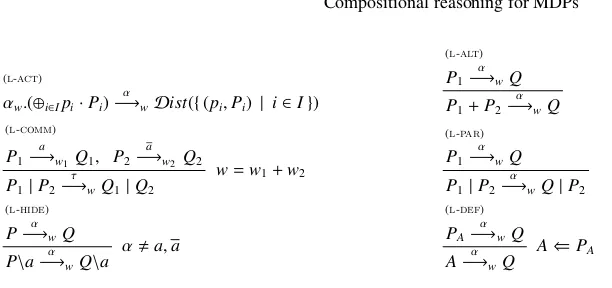
(l-act)

αw.(⊕i∈Ipi·Pi)

α

−→wDist({(pi,Pi) | i∈I})

(l-alt) P1

α

−→wQ

P1+P2 α

−→_wQ

(l-comm)

P1

a

−→w1 Q1, P2

a −→w2Q2

P1|P2 τ

−→wQ1|Q2

w=w1+w2

(l-par) P1

α

−→wQ

P1|P2 α

−→wQ|P2

(l-hide) P−→α wQ

P\a−→α _wQ\a α, a,a

(l-def) PA

α

−→wQ

A−→α _wQ

A⇐PA

Fig. 1.Weighted actions forCCMDP

This relies on the fact thatU down=⇒4 t1, which follows by transitivity, since we have already seen in Example 1 thatU=⇒τ ₃D.

Finallys0C2 s2because of the following simulation:

R = {(s0, hr,s2i)|r≥2} ∪ {(sd, hr, ∆i)|r≥0}

where∆is the distribution1₄·S+3₄·T. Note that∆down=⇒3s2although it is also possible

for it to do thedownaction for much less benefit. ut

The simulation relationsCrare defined coinductively. But in bounded wMDPS they can also be characterised inductively.

Definition 7. For every k≥0we define the relationCk_{⊆S ×(}

R≥0× D(S))as follows:

(i) C0_{=S ×(}

R≥0× D(S)) (ii) Ck+1_=S(Ck_{)for every k≥0.}

Finally we letC∞_beT∞

k=0 C

k_{. ut}

Theorem 3. In a bounded wMDP, the two relationsCandC∞coincide. ut Corollary 1 plays a crucial role in proving the above theorem.

The simplest approach to discussing compositionality is, as in [6], to introduce a process calculus-like syntax for wMDPs. Our calculus, called CCMDP, is based on CCS:

P::=αw.(⊕i∈Ipi·Pi) | P|P | P+P | 0 | P\a | A (2)

Intuitively, we view each process term as describing a wMDP. Formally we describe one overarching wMDP where the states are all termsP in the grammar (2) and the weighted actionsP−→α _w∆are those which can be derived by the rules in Figure 1; ob-vious symmetric counterparts to the rules (_l-_alt) (_l-_par) are omitted. In rule (_l-_act) we use the obvious notationDist({(pi,Pi) | i∈I}) for constructing a distribution from the formal term⊕_i∈Ipi·Pi. Note that all of the wMDPs described graphically in the In-troduction can be described inCCMDP. In the sequel we will not distinguish between the syntactic termP, its interpretation as a state in the wMDP defined in Figure 1, and the wMDP it induces by considering only those states, that is process terms, accessible from it.

Theorem 4 (Compositionality).The preordersCr, for each r∈R≥0, are preserved by

each of the operators in the languageCCMDP. ut

Example 3. LetP,Qbe two processes withPC0 Q. Consider the following processes: U⇐τ0.(τ1.U3

4⊕down1.Q) P0 ≡ up2.(down1.P1

4⊕down3.P) Q0 ≡ up2.U

By the analysis in Example 1 we know thatU=⇒τ ₃down1.Q, thusU down

=⇒₄ Q. Then it is easy to see thatdown1.PC0Uanddown3.PC0U. It follows from the compositionality ofC0that (down1.P1

4⊕down3.P)C0Uand furthermoreP

0_C

0 Q0. ut

3

A qualitative probabilistic logic

LetVarbe a set of variables, ranged over byX. Then we define the set of formulae as follows:

φ::=tt | ff | hαi

w(φ1p⊕φ2), α∈Actτ,w∈R≥0,p∈[0,1]

| φ1∧φ2 | φ1∨φ2 | X | minX. φ | maxX. φ

The two fixpoint operatorsminX.−andmaxX.−act as binders in the standard manner; we useL_Qto denote the set ofclosedformulae, that is containing no free variables. As a shorthand, we writehαi

wφforhαiw(φ1⊕φ

0_{) for anyφ}0_.

LetCondenote the set ofconfigurations, pairshr, ∆iwherer∈_R≥0and∆∈ D(S), withS denoting the state space of some wMDP. Intuitively this represents a system which has accumulated compensation r which it can use to satisfy formulae in the future. A formula fromLQ determines a set of configurations, those which satisfy it;

their calculation is standard, apart from the novel qualitative possibility operator. An environmentρis a function that maps each variable inVarto a subset ofCon. For a set V ⊆_R≥0× D(S) and a variableX ∈Var, we writeρ[X 7→V] for the environment that mapsXtoVandYtoρ(Y) for allY ,X. The semantics of a formulaφis given by the set of configurations[φ]_ρdefined as follows:

– [φ1∧φ2]ρ = [φ1]ρ∩[φ2]ρ, [φ1∨φ2]ρ = [φ1]ρ∪[φ2]ρ – [hαi

v(φ1p⊕φ2)]ρ = { hr, ∆i | ∆

α

=⇒_wΘwhere

h(r+w−v), Θi=hr1, Θ1ip⊕ hr2, Θ2iandhri, Θii ∈[φi]ρ} – [X]ρ = ρ(X)

– [minX. φ]_ρ = T_{{V |} [φ]

ρ[X7→V] ⊆ V} – [maxX. φ]_ρ = S_{{V | V ⊆} [φ]

ρ[X7→V]}

Whenφis closed the set[φ]_ρis independent of the environmentρ, and in this case we use the standard notationC |=φin place ofC ∈[φ].

The novel qualitative formulahαi

v(φ1p⊕φ2) represents the ability to do anαaction

with benefit at leastvand then probabilistically satisfy the propertyφ1p⊕φ2; we have hr, ∆i |= hαi

v(φ1 p⊕ φ2) whenever ∆

α

=⇒w Θ1 p⊕ Θ2 andhri, Θii |= φi for someri satisfying (r+w−v)=p·r1+(1−p)·r2. Here there are two possibilities:

(i) v>w: here the compensation comes into play. The action may be accepted despite being too heavy but the compensation for future use is reduced fromrtor−(v−w); this is split intor1, r2via the probabilityp. Note this possibility will only exist if r−(v−w)≥0.

(ii) v ≤w: The action is accepted and then the compensation is increased fromrto r+(w−v), which again is split proportionally intor1, r2, to satisfyφ1 andφ2 respectively.

Example 4. Both liveness and safety properties can be expressed inL_Q. For example, suppose AB denote the formulahai

0(hbi10tt 109⊕ tt) and C is a configuration. Then C |=ABmeans thatCcan perform anaaction such that at least 90% of the time it can subsequently perform abaction with a benefit of at least 10. So the formula

minX.hupi

0(hdowni10X 109⊕ tt) ∨ hupi0X

expresses the liveness property of being able to perform a sequence ofupactions to arrive at a state where at least 90% of the time adownaction for benefit at least 10 can be performed. On the other hand, the formula

maxX.hupi

0(hdowni10X 109⊕ tt) ∧ hstayi0X

expresses the safety property of always being able to perform astayaction and at the same time to perform anupaction to arrive at a state where at least 90% of the time a

downaction for benefit at least 10 can be performed. ut

LetLQ(r, ∆)={φ∈ LQ | hr, ∆i |=φ}. We have the following logical

characterisa-tion of simulacharacterisa-tions.

Theorem 5 (Logical characterisation). In a bounded wMDP, s Cr Θif and only if

LQ(0,s)⊆ LQ(r, Θ). ut

The proof of Theorem 5 exploits Theorem 3, which says thatCcan be approximated by a family of stratified relationsCk_fork∈

s

sr

sl

τ3

1 4

3 4

τ7

τ5

t

t2 t3

t4 t5

τ2

3 4

1 4

τ4

τ12

τ4

(a) (b)

Fig. 2.Testing systems

The import of Theorem 5 is that ifsCr Θdoes not hold then there is a formulaφ fromL_Q whichssatisfies butΘdoes not. Furthermore, it turns out that in a bounded wMDP this distinguishing formula will always be finite; that is contains no occurrence of a fixpoint operator. For example,s2 6C0 s0, where these are defined in the Introduc-tion, because of the distinguishing formulahupi

1(hdowni6tt 14⊕ hdowni2tt).

Our logic is expressive enough so that the whole behaviour of a state in a bounded wMDP can be captured by one formula in the logic:

Theorem 6 (Characteristic formula).In a bounded wMDP, for every state s there is acharacteristic formulaφ(s)∈ L_Qsuch that sCrΘif and only ifhr, Θi |=φ(s). ut

For example, the state s1 in the Introduction has the following characteristic formula:

φ(s1) = maxX.hupi₂(hdowni₁X 1

4⊕ hdowni3X).

4

Benefits based testing

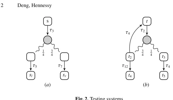
Standard theories of testing involve the idea of applying tests to processes and seeing if the result is a success. With the presence of weights in wMDPs we have a more elementary way of testing; we run them in parallel with other wMDPs and calculate the possible benefits which can be accrued. Then two wMDPs can be compared by examining the resulting sets of possible accrued benefits.

Consider the simple fully probabilistic wMDP in Figure 2(a), which results from running the testT =up1.down4.0in parallel with the systems1from the Introduction. Formally this is the sub-wMDP of the wMDP (s1|T) obtained by concentrating on the internal actionsτw; this is just the wMDP represented by (s1|T)\Actthat we denote by s1||T. Every time the experiment runs we get the initial benefit 3; three-quarters of the time we also get the benefit 7 while a quarter of time we get 5. So the total benefit is

3+3 4 ·7+

1

4 ·5=9.5.

which of its successors is chosen for execution, with the resulting set of benefits conse-quently depending on the choice of scheduler. Here we take a more abstract approach, following [4], and essentially allow arbitrary schedulers.

Definition 8 (Extreme derivatives).For any∆in a wMDP we write∆=⇒_wΦif – ∆=⇒_wΦ, that isΦis a hyper-derivative of∆

– Φisstable, that is s9τ for every s indΦe

where s9τ means that s cannot enable anyτ-transition. We sayΦis anextreme

deriva-tiveof∆, with weight w. ut

Intuitively every extreme derivation∆=⇒_wΦrepresents a computation from the initial distribution ∆guided by some implicit scheduler. For example, consider the hyper-derivation of an extreme derivative:

∆ = ∆→

0 +∆

×

0

∆→

0 τ −→_w

0∆

→

1 +∆

×

1

..

. (3)

∆→

k τ −→wk ∆

→

k₊1+∆

×

k+1

.. .

Φ =

∞ X

k=0

∆×

k

wherew=P

k≥0wk. Initially, since∆×₀ is stable,∆→₀ contains (in its support) all states which can proceed with the computation. The implicit scheduler decides for each of these states which step to take, cumulating in the first move,∆→₀ −→τ _w0∆→

1 +∆

×

1. At an arbitrary stage,∆→

k contains all states which can continue; the scheduler decides which step to take for each individual state and the overall result of the schedulers decision for this stage is captured in the step∆→

k τ −→_wk ∆→

k+1+∆

×

k+1.

Example 5. Referring to Figure 2(a) it is easy to see thatshas a unique (degenerate) extreme derivative,s1=⇒9.5 (₄1sl+3₄sr), intuitively representing the unique weighted computation froms1. However, consider the wMDP in Figure 2(b), in which there is a nondeterministic choice from statet2; here the extreme derivatives generated fromt, and their associated weights, will depend on the choices made during the computation by the implicit scheduler.

First suppose that the scheduler uses the static policy which mapst2 toh12,t4i. Then it is easy to see that the generated extreme derivative, which is degenerate, is t=⇒₁₂(3₄t4+1₄t5). However using the static policy which mapst2toh4,t1iwe gener-ate, using (3), a non-degenerate extreme derivative; after some calculations this can be seen to bet1=⇒24t5.

nondeterministically between them. But these are the only static policies and therefore we know from Theorem 1 that ift1=⇒w∆thenwmust take the formp·12+(1−p)·24 for some 0 ≤ p ≤ 1. That is the set of benefits which can be generated fromt1 is

{24−12·p | 0≤p≤1}. ut

Definition 9 (May testing).In a wMDP, for any∆∈ D(S), let

Benefits(∆)={w∈_R≥0 | ∆=⇒wΦ, for someΦ∈ Dsub(S)} Benefit sets are compared as follows:

B1≤rHoB2 if for every r1 ∈B1there exists some r2∈B2such that r1≤r+r2

For any two distributions∆, Θwe write∆vr

may Θif for every finite (testing) process T , Benefits(∆|| T)≤r

Ho Benefits(Θ|| T). We write∆ vmay Θto mean that there is some

r∈_R≥0such that∆vrmay Θ. ut

This interpretation of processes is inherently optimistic;∆vr

mayΘmeans that, given the investmentr, every possible benefit produced by∆can in principle be improved upon byΘ.

Note that in a bounded wMDPBenefits(∆) cannot contain∞. Moreover we can show that the parallel composition of a bounded wMDP with a finite wMDP is also bounded. This means that if we confine our attention to bounded wMDPs then benefit sets will always only contain real numbers. One way of restricting to bounded wMDPS is, by Theorem 2, to only use finitary convergent wMDPs.

Our first result shows that simulations can be used as a sound proof technique for this semantics:

Theorem 7 (Soundness).∆CrΘimplies∆vrmayΘ. ut The converse is not true in general:

Example 6. Consider the two distributions∆ =01

2⊕a1.0andΘ=τ2.012⊕a0.0. It is easy to see that∆6_C0 Θbecause there is no way to decomposeΘintoΘ1 1

2⊕Θ2for someΘ1, Θ2such thata1.0C0 Θ2. However, one can show that∆v0mayΘ. This follows from the observations below:

(i) For all weightwand testT,Benefits(τw.0||T) = {v+w|v∈Benefits(0||T)}. (ii) For all weightwand testT,Benefits(aw.0||T) ≤w_Ho Benefits(a0.0||T). Both assertions can be proved by structural induction onT.

Now supposew ∈ Benefits(∆ || T) for an arbitrary testT. There is some stable derivativeΓsuch that∆||T =⇒wΓ. It can be shown that there are somew1,w2, Γ1, Γ2 with0 || T =⇒w1 Γ1,a1.0 || T =⇒w2 Γ2,w =

1 2w1+

1

2w2, andΓ = 1 2 ·Γ1+

1 2 ·Γ2, where bothΓ1 andΓ2are stable. In other words, we havew1 ∈ Benefits(0 || T) and w2∈Benefits(a1.0||T). By (i) above,w1+2∈Benefits(τ2.0||T); by (ii) above, there exists somew0₂∈Benefits(a0.0||T) withw2≤w02+1. Thus, we can infer that

w= 1₂w1+1₂w2

< 1

2(w1+2)+ 1

2(w2−1) ≤ 1

2(w1+2)+ 1 2w

0

It turns out that1₂(w1+2)+1₂w0₂∈Benefits(Θ||T). Therefore, we have Benefits(∆||T) ≤0_Ho Benefits(Θ||T).

Since this reasoning is carried out for an arbitrary testT, it follows that∆v0

mayΘ. ut

Nevertheless we do have a testing characterisation for the unannotated simulation preorder:

Theorem 8 (Testing characterisation).In a bounded wMDP, sv_may Θif and only if svsimΘ.

Proof (Outline).One direction follows from Theorem 7. For the converse we carry out the proof in two steps: we first prove that s vr

may Θimplies the existence of some compensationr0 ≥ r such thatLQ(0,s) ⊆ LQ(r0, Θ), and then appeal to Theorem 5.

In the first step we proceed by constructing, for each formulaφ, a characteristic test T(φ), such that if a process satisfiesφthen it passes the testT(φ) with some threshold

benefit. ut

An alternative approach to testing would be to use one special actionωin a test to report success and when applying such a test to a system to report the weighted average of the weight of each path leading to an occurrence of the success action; this we refer to asexpected benefits testing. Here we will not give the formal definition of how these expected benefitsare calculated, which is provided in [3], but simply give an informal argument to show that our simulation preorder is not sound with respect to it.

Example 7 (Simulation is unsound for expected benefits testing).Consider the fol-lowing processes:

P=τ2.(01 4⊕a0.0) Q=τ1.(τ2.(01

2⊕a0.0)12⊕a0.0)

It is easy to see that P C0 Qsince the transitionP τ −→2 01

4⊕a0.0can be simulated by the hyper-derivativeQ =⇒τ ₂ 0 1

4⊕ a0.0. Now letT be the test ¯a0.ω. BothP || T andQ||Tgive rise to fully probabilistic wMDPs. The unique expected benefit resulted fromP||T is1₄·0+3₄·2, i.e.3₂. On the other hand, the unique expected benefit obtained fromQ||Tis1₂·1+1₂(1₂·0+1₂·3), i.e.5₄. As{3₂} 6≤0

Ho{ 5

4}, we have thatPis not related to Qunder expected benefits may testing; thusCis not sound for expected benefits testing. Note that if we consider total benefits, thenBenefits(P||T)={2}=Benefits(Q||T).

u t

5

Concluding remarks

wMDPs. It is shown to be a precongruence relation with respect to all structural oper-ators for constructing wMDPs from components. For finitary convergent wMDPs, we have also given logical and testing characterisations of the simulation preorder: it can be completely determined by a qualitative probabilistic logic and for each system we can find a characteristic formula to capture its behaviour; the simulation preorder also coincides with a notion of may testing preorder.

The dual of may testing is must testing. It would be interesting to investigate the must preorder given by our testing approach. We leave it as future work to provide a coinductive formulation of the preorder and study its logical characterisations.

There is a very limited literature on compositional theories of Markov decision pro-cesses particularly in the presence of weights. There is however an extensive literature on probabilistic variations of bisimulation equivalence for Markov chains; see Chapter 10 of [1] for an elementary introduction and [7] for a survey. Bisimulation equivalence has also been defined in [6] forInteractive Markov Chains (IMCs), and it is shown to be compositional, in the sense of our Theorem 4: it is preserved by the operators of a process calculus interpreted as IMCs.

There is also an extensive literature on weighted automata [5], and probabilistic variations have also been studied [2]. However there the focus is on traditional language theoretic issues, rather than our primary concern, compositionality.

References

1. C. Baier and J.-P. Katoen.Principles of Model Checking. The MIT Press, 2008.

2. K. Chatterjee, L. Doyen, and T.A. Henzinger. Probabilistic Weighted Automata. In Proc. CONCUR’09, LNCS 5710, pp. 244–258. Springer, 2009.

3. Y. Deng and M. Hennessy. Compositional reasoning for markov decision processes, 2010. Full version of the current paper. Available at http://basics.sjtu.edu.cn/˜yuxin/ temp/mdp.pdf.

4. Y. Deng, R. van Glabbeek, M. Hennessy, and C. Morgan. Testing finitary probabilistic pro-cesses. In Proc.CONCUR’09, LNCS 5710, pp. 274–288. Springer, 2009.

5. M. Droste, W. Kuich, and H. Vogler (Eds.)Handbook of Weighted Automata. Springer, 2009. 6. H. Hermanns. Interactive Markov Chains: The Quest for Quantified Quality, LNCS 2428.

Springer, 2002.

7. B. Jonsson, K.G. Larsen, and Y. Wang. Probabilistic Extensions of Process Algebras. In Handbook of Process Algebra, pp. 685–710. Elsevier, 2001.

8. A. Kiehn and S. Arun-Kumar. Amortised bisimulations. In Proc.FORTE’05, LNCS 3731, pp. 320–334. Springer, 2005.

9. M. Puterman.Markov Decision Processes. Wiley, 1994.

10. J. Rutten, M. Kwiatkowska, G. Norman, and D. Parker. Mathematical Techniques for Ana-lyzing Concurrent and Probabilistic Systems,P. Panangaden and F. van Breugel (eds.), vol-ume 23 ofCRM Monograph Series. American Mathematical Society, 2004.