Solution of Time-Dependent PDE Through Component-wise Approximation of Matrix Functions

Solution of Time-Dependent PDE Through

Component-wise Approximation of Matrix

Functions

James V. Lambers

Abstract—Block Krylov subspace spectral (KSS) methods are a “best-of-both-worlds” compromise be-tween explicit and implicit time-stepping methods for variable-coefficient PDE, in that they combine the ef-ficiency of explicit methods and the stability of im-plicit methods, while also achieving spectral accuracy in space and high-order accuracy in time. Block KSS methods compute each Fourier coefficient of the solu-tion using techniques developed by Gene Golub and G´erard Meurant for approximating elements of func-tions of matrices by block Gaussian quadrature in the spectral, rather than physical, domain. This paper demonstrates the superiority of block KSS methods, in terms of accuracy and efficiency, to other Krylov subspace methods in the literature. It is also de-scribed how the ideas behind block KSS methods can be applied to a variety of equations, including prob-lems for which Fourier spectral methods are not nor-mally feasible. In particular, the versatility of the ap-proach behind block KSS methods is demonstrated through application to nonlinear diffusion equations for signal and image processing, and adaptation to finite element discretization.

Keywords: spectral methods, Gaussian quadrature, block Lanczos, Maxwell’s equations, heat equation

1

Introduction

In [17] a class of methods, called block Krylov subspace spectral (KSS) methods, was introduced for the pur-pose of solving parabolic variable-coefficient PDE. These methods are based on techniques developed by Golub and Meurant in [8] for approximating elements of a function of a matrix by Gaussian quadrature in thespectraldomain. In [18], these methods were generalized to the second-order wave equation, for which these methods have ex-hibited even higher-order accuracy.

It has been shown in these references that KSS methods,

∗_{Submitted September 28, 2010. The University of}

Southern Mississippi, Department of Mathematics, Hatties-burg, MS 39406-0001 USA Tel/Fax: 601-266-5784/5818 Email: [email protected]

by employing different approximations of the solution op-erator for each Fourier coefficient of the solution, achieve higher-order accuracy in time than other Krylov subspace methods (see, for example, [14]) for stiff systems of ODE, and they are also quite stable, considering that they are explicit methods. They are also effective for solving sys-tems of coupled equations, such as Maxwell’s equations [23], and elliptic PDE such as Poisson’s equation or the Helmholtz equation [21].

In this paper, we review block KSS methods, and com-pare their performance to other Krylov subspace meth-ods from the literature. It is then shown that block KSS methods are applicable to PDE other than those best suited to Fourier spectral methods. Section 2 presents the approximation of bilinear forms involving functions of matrices by block Gaussian quadrature, as developed by Golub and Meurant. Section 3 describes how block KSS methods are built on this work, as applied to parabolic problems, and summarizes their main properties. Section 4 discusses implementation details, and demonstrates why KSS methods need to explicitly generate only one Krylov subspace, although information from several is used. In Section 5, we discuss modifications to block KSS methods in order to apply them to systems of cou-pled equations, such as Maxwell’s equations. Numerical results are presented in Section 6, in which block KSS methods are compared to other Krylov subspace meth-ods. In Section 7, block KSS methods are applied to nonlinear diffusion equations for signal and image pro-cessing. In Section 8, we discuss the adaptation of block KSS methods to bases other than the Fourier basis, which allows application to problems featuring complicated ge-ometries or more general boundary conditions. Conclu-sions and discussion of future work are in Section 9.

2

Elements of Functions of Matrices

In [8] Golub and Meurant describe a method for comput-ing quantities of the form

u𝑇𝑓(𝐴)v, (1)

IAENG International Journal of Applied Mathematics, 41:1, IJAM_41_1_01

whereuandvare𝑁-vectors,𝐴 is an𝑁×𝑁 symmetric positive definite matrix, and𝑓 is a smooth function.

The basic idea is as follows: since the matrix 𝐴is sym-metric positive definite, it has real eigenvalues

𝑏=𝜆1≥𝜆2≥ ⋅ ⋅ ⋅ ≥𝜆𝑁 =𝑎 >0, (2)

and corresponding orthogonal eigenvectors q𝑗, 𝑗 =

1, . . . , 𝑁. Therefore, the quantity (1) can be rewritten as

u𝑇𝑓(𝐴)v=

𝑁

∑

𝑗=1

𝑓(𝜆𝑗)u𝑇q𝑗q𝑇𝑗v. (3)

which can also be viewed as a Riemann-Stieltjes integral

u𝑇𝑓(𝐴)v=𝐼[𝑓] =

∫ 𝑏

𝑎

𝑓(𝜆)𝑑𝛼(𝜆). (4)

As discussed in [8], the integral𝐼[𝑓] can be approximated using Gaussian quadrature rules, which yields an approx-imation of the form

𝐼[𝑓] =

𝐾

∑

𝑗=1

𝑤𝑗𝑓(𝜆𝑗) +𝑅[𝑓], (5)

where the nodes 𝜆𝑗,𝑗 = 1, . . . , 𝐾, as well as the weights

𝑤𝑗, 𝑗 = 1, . . . , 𝐾, can be obtained using the symmetric

Lanczos algorithm ifu=v, and the unsymmetric Lanc-zos algorithm ifu∕=v (see [11]).

In the case u∕=v, there is a possibility that the weights may not be positive, which destabilizes the quadrature rule (see [2] for details). Instead, we consider

[

u v ]𝑇 𝑓(𝐴)[

u v ]

, (6)

which results in the 2×2 matrix

∫ 𝑏

𝑎

𝑓(𝜆)𝑑𝜇(𝜆) =

[

u𝑇_{𝑓(𝐴)u u}𝑇_𝑓(𝐴)v

v𝑇_{𝑓(𝐴)u v}𝑇_𝑓(𝐴)v

] , (7)

where𝜇(𝜆) is a 2×2 matrix function of 𝜆, each entry of which is a measure of the form𝛼(𝜆) from (4).

In [8] Golub and Meurant showed how a block method can be used to generate quadrature formulas. We will describe this process here in more detail. The integral

∫𝑏

𝑎 𝑓(𝜆)𝑑𝜇(𝜆) is now a 2×2 symmetric matrix and the

most general𝐾-node quadrature formula is of the form

∫ 𝑏

𝑎

𝑓(𝜆)𝑑𝜇(𝜆) =

𝐾

∑

𝑗=1

𝑊𝑗𝑓(𝑇𝑗)𝑊𝑗+𝑒𝑟𝑟𝑜𝑟, (8)

with 𝑇𝑗 and 𝑊𝑗 being symmetric 2×2 matrices. By

diagonalizing each𝑇𝑗, we obtain the simpler formula

∫ 𝑏

𝑎

𝑓(𝜆)𝑑𝜇(𝜆) = 2𝐾

∑

𝑗=1

𝑓(𝜆𝑗)v𝑗v𝑗𝑇+𝑒𝑟𝑟𝑜𝑟, (9)

where, for each𝑗,𝜆𝑗 is a scalar andv𝑗 is a 2-vector.

Each node𝜆𝑗 is an eigenvalue of the matrix

𝒯𝐾 =

⎡

⎢ ⎢ ⎢ ⎢ ⎢ ⎣

𝑀1 𝐵1𝑇

𝐵1 𝑀2 𝐵2𝑇

. ._. . ._. . ._.

𝐵𝐾−2 𝑀𝐾−1 𝐵𝐾𝑇−1

𝐵𝐾−1 𝑀𝐾

⎤

⎥ ⎥ ⎥ ⎥ ⎥ ⎦

, (10)

which is a block-triangular matrix of order 2𝐾. The vec-torv𝑗consists of the first two elements of the

correspond-ing normalized eigenvector. To compute the matrices𝑀𝑗

and 𝐵𝑗, we use the block Lanczos algorithm, which was

proposed by Golub and Underwood in [10].

3

Krylov Subspace Spectral Methods

We now review block KSS methods, which are easier to describe for parabolic problems. Let 𝑆(𝑡) = exp[−𝐿𝑡] represent the exact solution operator of the problem

𝑢𝑡+𝐿𝑢= 0, 𝑡 >0, (11)

𝑢(𝑥,0) =𝑓(𝑥), 0< 𝑥 <2𝜋, (12)

𝑢(0, 𝑡) =𝑢(2𝜋, 𝑡), 𝑡 >0. (13)

The operator 𝐿 is a second-order, self-adjoint, positive definite differential operator of the form

𝐿𝑢= (𝑝(𝑥)𝑢𝑥)𝑥+𝑞(𝑥)𝑢, (14)

where𝑝(𝑥)>0 and𝑞(𝑥)≥0 on [0,2𝜋]. It follows that𝐿

is self-adjoint and positive definite.

Let⟨⋅,⋅⟩denote the standard inner product of functions defined on [0,2𝜋]. Block Krylov subspace spectral meth-ods, introduced in [17], use Gaussian quadrature on the spectral domain to compute the Fourier coefficients of the solution. These methods are time-stepping algo-rithms that compute the solution at time𝑡1, 𝑡2, . . ., where

𝑡𝑛=𝑛Δ𝑡for some choice of Δ𝑡.

Given the computed solution ˜𝑢(𝑥, 𝑡𝑛) at time 𝑡𝑛, the

so-lution at time 𝑡𝑛+1 is computed by approximating the Fourier coefficients that would be obtained by applying the exact solution operator to ˜𝑢(𝑥, 𝑡𝑛),

ˆ

𝑢(𝜔, 𝑡𝑛+1) =

〈 ₁

√

2𝜋𝑒

𝑖𝜔𝑥_{, 𝑆(Δ𝑡)˜𝑢(𝑥, 𝑡} 𝑛)

〉

. (15)

This is accomplished by applying the approach from the previous section for approximating (1), with 𝐴 = 𝐿𝑁

where 𝐿𝑁 is a spectral discretization of 𝐿, 𝑓(𝜆) =

exp(−𝜆𝑡) for some𝑡, and the vectorsuandvare, respec-tively, ˆe𝜔andu𝑛, where ˆe𝜔is a discretization of √1_2𝜋𝑒𝑖𝜔𝑥

IAENG International Journal of Applied Mathematics, 41:1, IJAM_41_1_01

andu𝑛 is the approximate solution at time𝑡𝑛, evaluated

on an𝑁-point uniform grid.

For each wave number𝜔=−𝑁/2 + 1, . . . , 𝑁/2, we define

𝑅0(𝜔) =

[

ˆ

e𝜔 u𝑛

]

and compute the𝑄𝑅factorization

𝑅0(𝜔) =𝑋1(𝜔)𝐵0(𝜔). We then carry out block Lanczos iteration, applied to the discretized operator 𝐿𝑁, to

ob-tain a block tridiagonal matrix 𝒯𝐾(𝜔) of the form (10),

where each entry is a function of𝜔.

Then, we can express each Fourier coefficient of the ap-proximate solution at the next time step as

[ˆu𝑛+1]𝜔=[𝐵0𝐻𝐸

𝐻

12exp[−𝒯𝐾(𝜔)Δ𝑡]𝐸12𝐵0]₁₂ (16) where 𝐸12 =

[

e1 e2

]

. The computation of (16) con-sists of computing the eigenvalues and eigenvectors of

𝒯𝐾(𝜔) in order to obtain the nodes and weights for

Gaus-sian quadrature, as described earlier.

This algorithm has local temporal accuracy 𝑂(Δ𝑡2𝐾−1₎ [17]. Furthermore, block KSS methods are more accurate than the original KSS methods described in [20], even though they have the same order of accuracy, because the solutionu𝑛 _{plays a greater role in the determination}

of the quadrature nodes. They are also more effective for problems with oscillatory or discontinuous coefficients [17].

Block KSS methods are even more accurate for the second-order wave equation, for which block Lanczos it-eration is used to compute both the solution and its time derivative. In [18, Theorem 6], it is shown that when the leading coefficient is constant and the coefficient 𝑞(𝑥) is bandlimited, the 1-node KSS method, which has second-order accuracy in time, is also unconditionally stable. In general, as shown in [18], the local temporal error is

𝑂(Δ𝑡4𝐾−2_{) when𝐾 block Gaussian nodes are used.}

4

Implementation

KSS methods compute a Jacobi matrix corresponding to

eachFourier coefficient, in contrast to traditional Krylov subspace methods that normally use only a single Krylov subspace generated by the initial data or the solution from the previous time step. While it would appear that KSS methods incur a substantial amount of additional computational expense, that is not actually the case, be-cause nearly all of the Krylov subspaces that they com-pute are closely related by the wave number𝜔, in the 1-D case, or⃗𝜔= (𝜔1, 𝜔2, . . . , 𝜔𝑛) in the𝑛-D case.

In fact, the only Krylov subspace that is explicitly com-puted is the one generated by the solution from the pre-vious time step, of dimension (𝐾+ 1), where 𝐾 is the number of block Gaussian quadrature nodes. In

ad-dition, the averages of the coefficients of 𝐿𝑗, for 𝑗 = 0,1,2, . . . ,2𝐾−1, are required, where 𝐿 is the spatial differential operator. When the coefficients of 𝐿 are in-dependent of time, these can be computed once, during a preprocessing step. This computation can be carried out in𝑂(𝑁log𝑁) operations using symbolic calculus [19, 22].

With these considerations, the algorithm for a single time step of a 1-node block KSS method for solving (11), where

𝐿𝑢=−𝑝𝑢𝑥𝑥+𝑞(𝑥)𝑢, with appropriate initial conditions

and periodic boundary conditions, is as follows. We de-note the average of a function𝑓(𝑥) on [0,2𝜋] by𝑓, and the computed solution at time𝑡𝑛 by𝑢𝑛.

ˆ

𝑢𝑛=fft(𝑢𝑛),𝑣=𝐿𝑢𝑛, ˆ𝑣=fft(𝑣)

foreach𝜔 do

𝛼1=−𝑝𝜔2+𝑞(in preprocessing step)

𝛽1= ˆ𝑣(𝜔)−𝛼1𝑢ˆ𝑛(𝜔)

𝛼2=⟨𝑢𝑛, 𝑣⟩ −2 Re [ˆ𝑢𝑛(𝜔)𝑣(𝜔)] +𝛼1∣𝑢𝑛(𝜔)∣2

𝑒𝜔= [⟨𝑢𝑛, 𝑢𝑛⟩ − ∣𝑢ˆ𝑛(𝜔)∣2]1/2

𝑇𝜔=

[

𝛼1 𝛽1/𝑒𝜔

𝛽1/𝑒𝜔 𝛼2/𝑒2𝜔

]

ˆ

𝑢𝑛+1_{(𝜔) = [𝑒}−𝑇𝜔Δ𝑡_]11ˆ𝑢𝑛_{(𝜔) + [𝑒}−𝑇𝜔Δ𝑡_]12𝑒

𝜔

end

𝑢𝑛+1_{=ifft(ˆ𝑢}𝑛+1₎

It should be noted that for a parabolic problem such as (11), the loop over 𝜔 only needs to account for non-negligible Fourier coefficients of the solution, which are relatively few due to the smoothness of solutions to such problems.

5

Application to Maxwell’s Equations

We consider Maxwell’s equation on the cube [0,2𝜋]3_{, with} periodic boundary conditions. Assuming nonconductive material with no losses, we have

div ˆE= 0, div ˆH= 0, (17)

curl ˆE=−𝜇∂Hˆ

∂𝑡 , curl ˆH=𝜀 ∂Eˆ

∂𝑡, (18)

where ˆE, ˆHare the vectors of the electric and magnetic fields, and𝜀,𝜇are the electric permittivity and magnetic permeability, respectively.

Taking the curl of both sides of (18) yields

𝜇𝜀∂

2_Eˆ

∂𝑡2 = Δ ˆE+𝜇

−1_{curl ˆE× ∇𝜇, (19)}

𝜇𝜀∂

2_Hˆ

∂𝑡2 = Δ ˆH+𝜀

−1_{curl ˆH× ∇𝜀. (20)}

In this section, we discuss generalizations that must be made to block KSS methods in order to apply them to a

IAENG International Journal of Applied Mathematics, 41:1, IJAM_41_1_01

non-self-adjoint system of coupled equations such as (19). Additional details are given in [23].

First, we consider the following 1-D problem,

∂2u

∂𝑡2 +𝐿u= 0, 𝑡 >0, (21)

with appropriate initial conditions, and periodic bound-ary conditions, whereu: [0,2𝜋]×[0,∞)→ℝ𝑛for𝑛 >1,

and 𝐿(𝑥, 𝐷) is an𝑛×𝑛matrix where the (𝑖, 𝑗) entry is an a differential operator𝐿𝑖𝑗(𝑥, 𝐷) of the form

𝐿𝑖𝑗(𝑥, 𝐷)𝑢(𝑥) = 𝑚𝑖𝑗 ∑

𝜇=0

𝑎𝑖𝑗_𝜇(𝑥)𝐷𝜇𝑢, 𝐷= 𝑑

𝑑𝑥, (22)

with spatially varying coefficients𝑎𝑖𝑗𝜇,𝜇= 0,1, . . . , 𝑚𝑖𝑗.

Generalization of KSS methods to a system of the form (21) can proceed as follows. For𝑖, 𝑗= 1, . . . , 𝑛, let𝐿𝑖𝑗(𝐷)

be the constant-coefficient operator obtained by averag-ing the coefficients of 𝐿𝑖𝑗(𝑥, 𝐷) over [0,2𝜋]. Then, for

each wave number𝜔, we define𝐿(𝜔) be the matrix with entries𝐿𝑖𝑗(𝜔), i.e., the symbols of𝐿𝑖𝑗(𝐷) evaluated at𝜔.

Next, we compute the spectral decomposition of𝐿(𝜔) for each𝜔. For𝑗 = 1, . . . , 𝑛, let q𝑗(𝜔) be the Schur vectors

of 𝐿(𝜔). Then, we define our test and trial functions by

⃗

𝜙𝑗,𝜔(𝑥) =q𝑗(𝜔)⊗𝑒𝑖𝜔𝑥.

For Maxwell’s equations, the matrix𝐴𝑁 that discretizes

the operator

𝐴Eˆ = 1

𝜇𝜀 (

Δ ˆE+𝜇−1curl ˆE× ∇𝜇)

is not symmetric, and for each coefficient of the solu-tion, the resulting quadrature nodes 𝜆𝑗, 𝑗 = 1, . . . ,2𝐾,

from (9) are now complex and must be obtained by a straightforward modification of block Lanczos iteration for unsymmetric matrices.

6

Numerical Results

In this section, we compare the performance of block KSS methods with various methods based on exponential in-tegrators [13, 15, 30].

6.1

Parabolic Problems

We first consider a 1-D parabolic problem of the form (11), where the differential operator 𝐿 is defined by

𝐿𝑢(𝑥) =−𝑝𝑢′′(𝑥) +𝑞(𝑥)𝑢(𝑥),where𝑝≈0.4 and

𝑞(𝑥) ≈ −0.44 + 0.03 cos𝑥−0.02 sin𝑥+ 0.005 cos 2𝑥−

0.004 sin 2𝑥+ 0.0005 cos 3𝑥

is constructed so as to have the smoothness of a function with three continuous derivatives, as is the initial data

𝑢(𝑥,0). Periodic boundary conditions are imposed.

We solve this problem using the following methods:

∙ A 2-node block KSS method. Each time step re-quires construction of a Krylov subspace of dimen-sion 3 generated by the solution, and the coefficients of 𝐿2 and 𝐿3 are computed during a preprocessing step.

∙ A preconditioned Lanczos iteration for approximat-ing 𝑒−𝜏 𝐴v, introduced in [24] for approximating the matrix exponential of sectorial operators, and adapted in [30] for efficient application to the so-lution of parabolic PDE. In this approach, Lanczos iteration is applied to (𝐼+ℎ𝐴)−1_{, whereℎis a} param-eter, in order to obtain a restricted rational approxi-mation of the matrix exponential. We use𝑚= 4 and

𝑚= 8 Lanczos iterations, and chooseℎ= Δ𝑡/10, as in [30].

∙ A method based on exponential integrators, from [13], that is of order 3 when the Jacobian is approx-imated to within 𝑂(Δ𝑡). We use 𝑚 = 8 Lanczos iterations.

Since the exact solution is not available, the error is es-timated by taking the ℓ2-norm of the relative difference between each solution, and that of a solution computed using a smaller time step Δ𝑡 = 1/64 and the maximum number of grid points.

The results are shown in Figure 1. As the number of grid points is doubled, only the block KSS method shows an improvement in accuracy; the preconditioned Lanc-zos method exhibits a slight degradation in performance, while the explicit fourth-order exponential integrator-based method requires that the time step be reduced by a factor of 4 before it can deliver the expected order of convergence; similar behavior was demonstrated for an explicit 3rd-order method from [14] in [20].

The preconditioned Lanczos method requires 8 Lanczos iterations to match the accuracy of a block KSS method that uses only 2. On the other hand, the block KSS method incurs additional expense due to (1) the compu-tation of the moments of𝐿, for each Fourier coefficient, and (2) the exponentiation of separate Jacobi matrices for each Fourier coefficient. These expenses are mitigated by the fact that the first takes place once, during a prepro-cessing stage, and both tasks require an amount of work that is proportional not to the number of grid points, but to the number of non-negligible Fourier coefficients of the solution.

IAENG International Journal of Applied Mathematics, 41:1, IJAM_41_1_01

Figure 1: Estimates of relative error at 𝑡 = 0.1 in solu-tions of (11) computed using preconditioned exponential integrator [30] with 4 and 8 Lanczos iterations, a 4th-order method based on an exponential integrator [15], and a 2-node block KSS method. All methods compute solutions on an𝑁-point grid, with time step Δ𝑡, for var-ious values of 𝑁 and Δ𝑡.

6.2

Maxwell’s Equations

We now apply a 2-node block KSS method to (19), with initial conditions

ˆ

E(𝑥, 𝑦, 𝑧,0) =F(𝑥, 𝑦, 𝑧), ∂

ˆ

E

∂𝑡(𝑥, 𝑦, 𝑧,0) =G(𝑥, 𝑦, 𝑧),

(23) with periodic boundary conditions. The coefficients 𝜇

and𝜀are given by

𝜇(𝑥, 𝑦, 𝑧) = 0.4077 + 0.0039 cos𝑧+ 0.0043 cos𝑦−

0.0012 sin𝑦+ 0.0018 cos(𝑦+𝑧) + 0.0027 cos(𝑦−𝑧) + 0.003 cos𝑥+ 0.0013 cos(𝑥−𝑧) + 0.0012 sin(𝑥−𝑧) + 0.0017 cos(𝑥+𝑦) + (24) 0.0014 cos(𝑥−𝑦), (25)

𝜀(𝑥, 𝑦, 𝑧) = 0.4065 + 0.0025 cos𝑧+ 0.0042 cos𝑦+ 0.001 cos(𝑦+𝑧) + 0.0017 cos𝑥+ 0.0011 cos(𝑥−𝑧) + 0.0018 cos(𝑥+𝑦) + 0.002 cos(𝑥−𝑦). (26)

The components of Fand G are generated in a similar fashion, except that the 𝑥- and𝑧-components are zero.

We use a block KSS method that uses 𝐾 = 2 block quadrature nodes per coefficient in the basis described in Section 5, that is 6th-order accurate in time, and a

cosine method based on a Gautschi-type exponential in-tegrator [13, 15]. This method is second-order in time, and in these experiments, we use 𝑚 = 2 Lanczos itera-tions to approximate the Jacobian. It should be noted that when 𝑚 is increased, even to a substantial degree, the results are negligibly affected.

Figure 2 demonstrates the convergence behavior for both methods. At both spatial resolutions, the block KSS method exhibits approximately 6th-order accuracy in time as Δ𝑡decreases, except that for𝑁 = 16, the spatial error arising from truncation of Fourier series is signifi-cant enough that the overall error fails to decrease below the level achieved at Δ𝑡 = 1/8. For 𝑁 = 32, the so-lution is sufficiently resolved in space, and the order of overgence as Δ𝑡→0 is approximately 6.1.

We also note that increasing the resolution does not pose any difficulty from a stability point of view. Unlike ex-plicit finite-difference schemes that are constrained by a CFL condition, KSS methods do not require a reduction in the time step to offset a reduction in the spatial step in order to maintain boundedness of the solution, because their domain of dependence includes the entire spatial domain for any Δ𝑡.

Figure 2: Estimates of relative error at 𝑡 = 1 in solu-tions of (19), (23) computed using a cosine method based on a Gautschi-type exponential integrator [13, 15] with 2 Lanczos iterations, and a 2-node block KSS method. Both methods compute solutions on an 𝑁3_{-point grid,} with time step Δ𝑡, for various values of𝑁 and Δ𝑡.

The Gautschi-type exponential integrator method is second-order accurate, as expected, and delivers nearly identical results for both spatial resolutions, but even with a Krylov subspace of much higher dimension than that used in the block KSS method, it is only able to achieve at most second-order accuracy, whereas a block

IAENG International Journal of Applied Mathematics, 41:1, IJAM_41_1_01

KSS method, using a Krylov subsapce of dimension 3, achieves sixth-order accuracy. This is due to the incorpo-ration of the moments of the spatial differential operator into the computation, and the use of Gaussian quadra-ture rules specifically tailored to each Fourier coefficient.

7

Other Spatial Discretizations

The main idea behind KSS methods, that higher-order accuracy in time can be obtained by componentwise ap-proximation, is not limited to the enhancement of spec-tral methods that employ Fourier basis functions. Let

𝐴 be an 𝑁 ×𝑁 matrix and 𝑓 be an analytic function. Then 𝑓(𝐴)v can be computed efficiently by approxima-tion of each component, with respect to an orthonormal basis{u𝑗}𝑁𝑗=1, by a 𝐾-node Gaussian quadrature rule if expressions of the form

u𝐻_𝑗 𝐴𝑘u𝑗, u𝐻𝑗 𝐴

𝑘_{v, v}𝐻_𝐴𝑘_{v (27)}

can be computed efficiently for 𝑗 = 1, . . . , 𝑁 and 𝑘 = 0, . . . ,2𝐾 − 1, and transformation between the basis

{u𝑗}𝑁𝑗=1 and the standard basis can be performed effi-ciently.

The first expression in (27) can be computed in a prepro-cessing stage if the operator discretized by𝐴is indepen-dent of time, or it can be computed analytically if the members of the basis {u𝑗}𝑁𝑗=1 can be simply expressed in terms of 𝑗, as in Fourier spectral methods. The other two expressions in (27) are readily obtained from bases for Krylov subspaces generated by v. Thus it is worth-while to explore the adaptation of KSS methods to other spatial discretizations for which the recursion coefficients can be computed efficiently. The temporal order of ac-curacy achieved in the case of Fourier spectral methods is expected to apply to such discretizations, as only the measures in the Riemann-Stieltjes integrals are changing, not the integrands.

Consider a general PDE of the form𝑢𝑡=𝐿𝑢on a domain

Ω, with appropriate initial and boundary conditions. A finite element discretization results in a system of ODEs of the form𝑀u𝑡=𝐾u+F, where𝑀 is the mass matrix,

𝐾 is the stiffness matrix,F is the load vector, and uis a vector of coefficients of the approximate solution in the basis of trial functions. Because𝑀 and𝐾are sparse, our approach can be used to compute bilinear forms involving functions of𝑀−1_{𝐾, where the basis vectorsu}

𝑗 are

sim-ply the standard basis vectors. Through mass lumping,

𝑀 can be replaced by a diagonal matrix in a way that preserves spatial accuracy [16].

We now present some algorithmic details. Let 𝐴 be a symmetric positive definite matrix. For𝑗= 1, . . . , 𝑁, we approximate e𝑇_𝑗 exp[−𝐴𝑡]f using the following algorithm

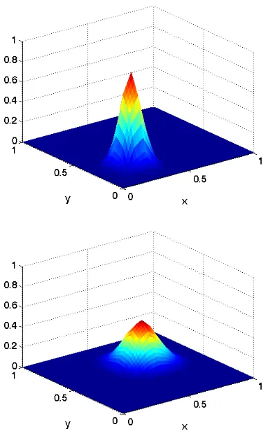
Figure 3: Solution at𝑡= 0 (top) and𝑡= 0.5 (bottom).

based on block Lanczos iteration. First, we perform the following initializations:

𝑋0 = 0 (28)

𝑅0 =

[ e𝑗 f

]

. (29)

Next, we let 𝐾 denote the number of block Gaussian quadrature nodes to be used for each component. Then, for𝑘= 1, . . . , 𝐾, we compute the following:

𝑅𝑘−1 = 𝑋𝑘Γ𝑘−1 (QR factorization) (30)

𝑀𝑘 = 𝑋𝑘𝑇𝐴𝑋𝑘 (31)

𝑅𝑘 = 𝐴𝑋𝑘−𝑋𝑘𝑀𝑘−𝑋𝑘−1Γ𝑘−1 (32) Next, we compute the block tridiagonal matrix 𝒯𝐾 as

in (10). Finally, we approximate each component of the solution as in (16):

e𝑇𝑗 exp[−𝐴𝑡]f ≈e 𝑇

1Γ

𝑇

0𝐸

𝑇

12exp[−𝑇𝐾𝑡]𝐸12Γ0e2. The challenge is to efficiently compute the elements of

𝑇𝐾 for all𝑗= 1, . . . , 𝑁.

IAENG International Journal of Applied Mathematics, 41:1, IJAM_41_1_01

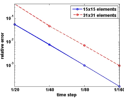
Figure 4: Relative error at𝑡= 0.5 at various time steps.

To that end, we now consider an alternative approach to describing block Lanczos iteration, applied to all compo-nents simultaneously. We define

𝑅0=[ 𝐼 fe𝑇 ], (33) whereeis an𝑁-vector of all ones. Then, we define

𝑅0=𝑋1Γ0 (34)

where Γ0is a 2𝑁×2𝑁 matrix with block structure

Γ0=

[

Γ11 0 Γ120 0 Γ22 0

]

. (35)

Each block is a diagonal matrix. The entries of these blocks satisfy

[

[𝑅0]𝑗 [𝑅0]𝑗+𝑁 ] = [ [𝑋1]𝑗 [𝑋1]𝑗+𝑁 ]×

[

[Γ0]𝑗𝑗 [Γ0]𝑗,𝑗+𝑁

[Γ0]_{𝑗+𝑁,𝑗} [Γ0]𝑗+𝑁,𝑗+𝑁

] ,

(36)

for 𝑗 = 1, . . . , 𝑁. Because this factorization is actually a QR factorization of columns 𝑗 and 𝑗+𝑁 of 𝑅0, the (2,1)-block of Γ0, Γ21𝑖 , is zero. The remaining entries can

be computed as follows. We write

𝑅0=

[

𝑅01 𝑅02

]

, 𝑋1=

[

𝑋11 𝑋12

]

, (37)

and then obtain

Γ110 = diag(e

𝑇

[𝑅01∗𝑅01])1/2 (38)

𝑋11 = 𝑅01[Γ110 ]

−1 ₍₃₉₎

Γ12₀ = [Γ11₀ ]−1diag(e𝑇[𝑅01∗𝑅02]) (40)

𝑌12 = 𝑅02−𝑅01[Γ110 ]

−1_Γ12

0 (41)

Γ22₀ = diag(e𝑇[𝑌12∗𝑌12])1/2 (42)

𝑋12 = 𝑌12[Γ220 ]−1 (43)

where we denote the componentwise products of matrices

𝐴and𝐵 by𝐴∗𝐵.

Next, we define

𝑀1= (𝑋1𝑇𝐴𝑋1)∗(𝐸2⊗𝐼𝑁), (44)

where𝐸2 is a 2×2 matrix of ones, and𝐼𝑁 is the𝑁×𝑁

identity matrix. In other words,𝑀1is a 2𝑁×2𝑁 matrix that is a 2×2 matrix of diagonal blocks, where each block is the diagonal of the corresponding block of 𝑋𝑇

1𝐴𝑋1. It should be noted that 𝑀1 can be computed without forming𝑋𝑇

1𝐴𝑋1 in its entirety. From

[𝑀1]𝑖𝑗=𝛿𝑖mod𝑁,𝑗mod𝑁 𝑁

∑

𝑘,ℓ=1

[𝑋1]𝑘𝑖𝐴𝑘ℓ[𝑋1]ℓ𝑗, (45)

and (37), we obtain

𝑀1=

[

diag(e𝑇_[𝑋

11∗𝑌11]) diag(e𝑇[𝑋11∗𝑌12)] diag(e𝑇_[𝑋

12∗𝑌11]) diag(e𝑇[𝑋12∗𝑌12)]

] ,

𝑌11=𝐴𝑋11, 𝑌12=𝐴𝑋12.

The remaining blocks 𝑀𝑘, 𝑘 = 2, . . . , 𝐾, can be

com-puted in a similar fashion. The matrices 𝑅1, . . . , 𝑅𝐾−1 can be computed by standard matrix multiplication, tak-ing sparisty into account. The matrices𝑋2, . . . , 𝑋𝐾 and

Γ2, . . . ,Γ𝐾−1 can be computed by carrying out the 𝑄𝑅 factorization as in (38)-(43).

Once the matrices 𝑀𝑘 and Γ𝑘 are computed, we can

compute the matrices 𝒯𝐾, as defined in (10), for each

component of the solution. Each of these matrices is 2𝐾×2𝐾. From its eigenvalues and eigenvectors, we ob-tain the nodes and weights for block Gaussian quadrature that enable us to approximate the appropriate component of the solution.

As an example of the applicability of block Gaussian quadrature to spatial discretizations other than a Fourier spectral discretization, an adaptation of a 2-node block KSS method is used to solve an advection-diffusion prob-lem on the rectangle (0,1)2_{, in which the flow is being} advected from the origin at a 45-degree angle. The ini-tial data is Gaussian, with homogeneous Dirichlet inflow boundary conditions, and homogeneous Neumann out-flow boundary conditions. The Peclet number is 200. A 15×15 uniform mesh and piecewise bilinear basis func-tions are used. The results are shown in Figures 3 and 4. As in the Fourier spectral case, the adapted KSS method is 3rd-order accurate in time. We see that KSS methods can be just as effective for time-stepping in finite element models, such as that described in [28], as in Fourier spec-tral methods

IAENG International Journal of Applied Mathematics, 41:1, IJAM_41_1_01

8

Nonlinear Diffusion for Signal and

Im-age Processing

In [12], Guidotti and the author introduced the nonlinear diffusion equation

𝑢𝑡− ∇ ⋅(𝑔(𝑢)∇𝑢) = 0, (46)

𝑔(𝑢) = 1

1 +𝑐2_∣∇1−𝜀_𝑢∣2, 0< 𝜖 <1. (47) The diffusion coefficient𝑔(𝑢) involves a slight weakening of the nonlinearity featured in the well-known Perona-Malik equation [26] for sharpening and denoising images, in order to overcome its drawbacks of being ill-posed and susceptible to “staircasing” effects [12], without introduc-ing blurrintroduc-ing, as some regularizations of Perona-Malik do [1, 5].

For diffusion equations such as (46), (47) it is generally not practical to use explicit time-stepping methods, be-cause of the severe constraints they impose on the time step. A straightforward alternative is to use implicit time-stepping in conjunction with an iterative method such as MINRES [25]. However, this approach has not been found to be efficient, and solutions tend to exhibit staircasing and high-frequency oscillations.

These effects are illustrated by solving (46), (47) in one space dimension, with initial data equal to a character-istic function convolved with a Gaussian kernel. The re-sults are shown in Figure 5. As the signal sharpens, the solution exhibits staircasing and high-frequency oscilla-tions, which are eventually eliminated over time.

Figure 5: Sharpening of a smooth function, using𝑐= 1,

𝜀 = 0.1, Δ𝑡 = 0.0003. Left plot: backward Euler with MINRES for time-stepping. Right plot: KSS method.

To demonstrate the effectiveness of KSS methods for im-age processing applications, the same problem is solved with a 1-node KSS method. As seen in Figure 5, the previously observed staircasing and high-frequency oscil-lations do not occur.

We then illustrate the use of block KSS methods in de-noising of images. Here the application (46) is

inves-tigated in the context of color images for which 𝑢 ∈

ℝ3. The experiments performed were not limited to a

channel-by-channel generalization of (46), but the best results were obtained for such a choice. It would also conceivably be best to choose the contstant𝑐taylored to each channel𝑢𝑖_{, 𝑖= 1,2,3. Once more experiments}

de-liver the best results when the constants are chosen equal to give

{𝑢𝑖_𝑡− ∇ ⋅

( ₁

1 +𝑐∣∇1−𝜀_𝑢𝑖_∣2∇𝑢

𝑖

)

= 0, 𝑢𝑖(0) =𝑢𝑖₀, (48)

for𝑖= 1,2,3.

In order to make sense of this model, the fractional gradi-ent appearing in the equations needs to be defined. It is convenient (but not necessary) to work with doubly peri-odic functions (non periperi-odic images can always be made periodic by appropriate reflection across the boundaries as to avoid boundary effects. Then one has

∂𝑧=ℱ𝑧−1diag

[

2𝜋𝑖𝑘𝑧]ℱ𝑧, 𝑧=𝑥, 𝑦 ,

whereℱ denotes the discrete Fourier transform. The the

fractional gradient is defined as∇𝜌₌

[ ∂𝜌

𝑥

∂𝜌 𝑦

]

, where

∂_𝑧𝜌=ℱ−1

𝑧 diag

[

(2𝜋𝑖𝑘𝑧)𝜌

]

ℱ𝑧, 𝑧=𝑥, 𝑦 .

The exponentiation of Λ𝑧;𝑛,𝑛 is carried out as follows:

(𝑖𝑘)1−𝜀=∣𝑘∣1−𝜀_𝑒𝑖𝜋/2(1−𝜀)sign(𝑘)_{, 𝑘=−𝑛/2+1, . . . , 𝑛/2.}

We now apply this model to a test image that is 256×256. The noise is Gaussian, with standard deviation of 11%. The result is shown in Figure 6. We observe that the noise is removed over a very short interval in time, without any visible artifacts, blurring or loss of contrast.

Figure 6: Denoising of L.A. aerial photo with 𝜖 = 0.1,

𝑐= 0.5 and𝑇 = 1.5×10−4

Block KSS methods also effective as a time-stepping scheme for reaction-diffusion equations that are used to

IAENG International Journal of Applied Mathematics, 41:1, IJAM_41_1_01

achieve sharpening of images via deconvolution, such as

𝑢𝑡=∇ ⋅(𝑔(𝑢)∇𝑢))−𝛼˜ℎ∗(ℎ∗𝑢−𝑓), (49)

where ℎ is a blurring kernel and ˜ℎ is the mirror kernel ˜

ℎ(𝑥, 𝑦)≡ℎ(−𝑥,−𝑦). This equation is a modification of an equation introduced in [31], with the diffusion coef-ficient defined in (47). A 1-node block KSS method is applied to the convolution of a flower-shaped characteris-tic function,with a Gaussian kernel, resulting in a blurred image.The original and blurred images, as well as the re-sult of the deconvolution, are shown in Figure 7.

Figure 7: Left plot: Original image defined via flower-shaped characteristic function. Center plot: Blurred flower image obtained by convolution with kernel

ℎ(𝑥, 𝑦) =𝑒−100(𝑥2+𝑦2). Right plot: Deblurred flower im-age obtained by solving (49) to time𝑇 = 0.3 with𝜖= 0.1,

𝑐= 0.01, Δ𝑡= 0.0002, and𝛼= 104.

It should be noted that the use of iterative methods such as MINRES necessitates that larger images are handled by decomposing them into blocks of a manageable size, such as 128×128, and denoised independently of one another. When using periodic boundary conditions, a “padding” border must be added around each block, re-flecting the image across its boundary as needed, in or-der to prevent artifacts from appearing at the interfaces between blocks or on the boundary of the entire image. Unfortunately, when integrating over longer periods of time, mismatches at the interfaces between blocks can still appear. The block KSS method, on the other hand, is capable of efficiently denoising larger images without such decomposition, thus circumventing these implemen-tation difficulties.

The approach used to model this kind of fractional dif-fusion equation can readily be applied to other equations involving fractional spatial differentiation, such as in [4].

9

Summary and Future Work

We have demonstrated that block KSS methods can be applied to Maxwell’s equations with smoothly varying coefficients, by appropriate generalization of their ap-plication to the scalar second-order wave equation, in a

way that preserves the order of accuracy achieved for the wave equation. Furthermore, it has been demonstrated that while traditional Krylov subspace methods based on exponential integrators are most effective for parabolic problems, especially when aided by preconditioning as in [30], KSS methods perform best when applied to hy-perbolic problems, in view of their much higher order of accuracy.

Future work will extend the approach described in this paper to more realistic applications involving Maxwell’s equations, and related models such as the Vlasov-Maxwell-Fokker-Planck system [7], by using symbol mod-ification to efficiently implement perfectly matched layers (see [3]) for simulation on infinite domains, and various techniques (see [6, 29]) to effectively handle discontin-uous coefficients. In addition, block KSS methods will be adapted to work with bases of Chebyshev polynomi-als for problems with non-homogeneous boundary condi-tions, including nonlocal boundary conditions as in [27].

References

[1] Alvarez, L., Lions, P.-L., Morel, J.-M.: Image se-lective smoothing and edge-detection by non-linear diffusion. II. SIAM J. Numer. Anal. 29(3) (1991) 845-866.

[2] Atkinson, K.: An Introduction to Numerical Anal-ysis, 2nd Ed.Wiley (1989)

[3] Berenger, J,: A perfectly matched layer for the ab-sorption of electromagnetic waves.J. Comp. Phys. 114(1994) 185-200.

[4] Blackledge, J. M.: Application of the Fractional Dif-fusion Equation for Predicting Market Behaviour.

IAENG Journal of Applied Mathematics 40(3) (2010) 23-51.

[5] Catt´e, F., Lions, P.-L., Morel, J.-M., Coll, T.: Im-age selective smoothing and edge-detection by non-linear diffusion.SIAM J. Numer. Anal.29(1) (1992) 182-193.

[6] Gelb, A., Tanner, J.: Robust Reprojection Methods for the Resolution of the Gibbs Phenomenon.Appl. Comput. Harmon. Anal.20(2006) 3-25.

[7] El Ghani, N.: Diffusion Limit for the Vlasov-Maxwell-Fokker-Planck System.IAENG Journal of Applied Mathematics40(3) (2010) 52-59.

[8] Golub, G. H., Meurant, G.: Matrices, Moments and Quadrature. Proceedings of the 15th Dundee Con-ference, June-July 1993, Griffiths, D. F., Watson, G. A. (eds.), Longman Scientific & Technical (1994)

IAENG International Journal of Applied Mathematics, 41:1, IJAM_41_1_01

[9] Golub, G. H., Gutknecht, M. H.: Modified Moments for Indefinite Weight Functions.Numerische Math-ematik57(1989) 607-624.

[10] Golub, G. H., Underwood, R.: The block Lanc-zos method for computing eigenvalues. Mathemati-cal Software III, J. Rice Ed., (1977) 361-377.

[11] Golub, G. H, Welsch, J.: Calculation of Gauss Quadrature Rules.Math. Comp.23(1969) 221-230.

[12] Guidotti, P., Lambers, J. V.: Two New Nonlinear Nonlocal Diffusions for Noise Reduction.J. of Math. Imaging Vis.33(2009) 27-35.

[13] Hochbruck, M., Lubich, C.: A Gautschi-type method for oscillatory second-order differential equations, Numerische Mathematik 83 (1999) 403-426.

[14] Hochbruck, M., Lubich, C.: On Krylov Subspace Approximations to the Matrix Exponential Opera-tor.SIAM Journal of Numerical Analysis34(1997) 1911-1925.

[15] Hochbruck, M., Lubich, C., Selhofer, H.: Expo-nential Integrators for Large Systems of Differential Equations. SIAM Journal of Scientific Computing 19(1998) 1552-1574.

[16] Hughes, T. J. R.: The Finite Element Method: Lin-ear Static and Dynamic Finite Element Analysis. Dover (2000).

[17] Lambers, J. V.: Enhancement of Krylov Sub-space Spectral Methods by Block Lanczos Iteration.

Electronic Transactions on Numerical Analysis 31

(2008) 86-109.

[18] Lambers, J. V.: An Explicit, Stable, High-Order Spectral Method for the Wave Equation Based on Block Gaussian Quadrature.IAENG Journal of Ap-plied Mathematics38(4) (2008) 333-348.

[19] Lambers, J. V.: Krylov Subspace Spectral Methods for the Time-Dependent Schr¨odinger Equation with Non-Smooth Potentials. Numerical Algorithms 51

(2009) 239-280.

[20] Lambers, J. V.: Krylov Subspace Spectral Meth-ods for Variable-Coefficient Initial-Boundary Value Problems. Electronic Transactions on Numerical Analysis20(2005) 212-234.

[21] Lambers, J. V.: A Multigrid Block Krylov Sub-space Method for Variable-Coefficient Elliptic PDE.

IAENG Journal of Applied Mathematics 39(4) (2009) 236-246.

[22] Lambers, J. V.: Practical Implementation of Krylov Subspace Spectral Methods. Journal of Scientific Computing32(2007) 449-476.

[23] Lambers, J. V.: A Spectral Time-Domain Method for Computational Electrodynamics. Adavances in Applied Mathematics and Mechanics 1(2009) 781-798.

[24] Moret, I., Novati, P.: RD-rational approximation of the matrix exponential operator. BIT44 (2004) 595-615.

[25] Paige, C. C., Saunders, M. A.: Solution of Sparse Indefinite Systems of Linear Equations. SIAM J. Numer. Anal.12(1975) 617-629.

[26] Perona, P., Malik, J.: Scale-space and edge detec-tion using anisotropic diffusion.IEEE Pattern Anal. Mach. Intell.12 (1990) 161-192.

[27] Siddique, M.: Numerical Computation of Two-dimensional Diffusion Equation with Nonlocal Boundary Conditions. IAENG Journal of Applied Mathematics40(1) (2010) 26-31.

[28] Tewari, S. G., Pardasani, K. R.: Finite Element Model to Study Two Dimensional Unsteady State Cytosolic Calcium Diffusion in Presence of Excess Buffers. IAENG Journal of Applied Mathematics 40(3) (2010) 1-5.

[29] Vallius, T., Honkanen, M.: Reformulation of the Fourier nodal method with adaptive spatial resolu-tion: application to multilevel profiles. Opt. Expr. 10(1) (2002) 24-34.

[30] van den Eshof, J., Hochbruck, M.: Preconditioning Lanczos approximations to the matrix exponential.

SIAM Journal of Scientific Computing 27 (2006) 1438-1457.

[31] Welk, M., Theis, D., Brox, T., Weickert, J.: PDE-Based Deconvolution with Forward-Backward Dif-fusivities and Diffusion Tensors. In Scale Space 2005, Kimmel, R., Sochen, N., Weickert, J. (eds.) Springer (2005) 585-597.

IAENG International Journal of Applied Mathematics, 41:1, IJAM_41_1_01