Abstract— The efficiency of several preconditioned Conjugate Gradient (PCG) schemes for solving of large sparse linear systems arising from application of interior point methods to nonlinear Finite Element Limit Analysis (FELA) is studied. Direct solvers fail to solve these linear systems in large sizes, such as large 2D and 3D problems, due to their high storage and computational cost. This motivates using iterative methods. However, iterative solvers are not efficient for difficult problems without preconditioning techniques. In this paper, the effect of various preconditioning techniques on the convergence behavior of the preconditioned Conjugate Gradient (PCG) is investigated through a detailed comparative study. Furthermore, numerical results of applying PCG to several sample systems are presented and discussed thoroughly in a parametric study. Our results suggest that while incomplete Cholesky preconditioners are by far the most efficient techniques for sequential computations, significant gains may result from use of sparse approximate inverse methods in parallel environment in this field.
Index Terms— incomplete Cholesky factorization, approximate inverse preconditioner, limit analysis, preconditioned conjugate gradient method, cone programming
I. INTRODUCTION
The application of second order cone programming (SOCP) to solving optimization problems arising in Geomechanics has recently been of growing interest and significant advances have been made in this field. Some of the most important applications include traditionally difficult problems in plasticity [24], finite element limit analysis [26] and most recently granular contact dynamics [25]. In this paper, we focus on the case of finite element limit analysis (FELA). Upon formulating the original problem as SOCP, it can be solved by primal-dual interior point method (IPM). An efficient IPM algorithm for conic quadratic optimization was proposed by Anderson et al [2]. However, in each step of this method, a symmetric positive definite (SPD) linear system of equation needs to be solved. Due to their robustness and accuracy, the direct solvers have been traditionally used for this task [2], [38].
O. Kardani is with the Center for Geotechnical and Materials Modelling, University of Newcastle, NSW, Australia (phone: +612-4921-5842; e-mail: Omid.Kardani@ uon.edu.au).
A. V. Lyamin is with the Center for Geotechnical and Materials Modelling, University of Newcastle, NSW, Australia (e-mail: [email protected]).
K. Krabbenhøft is with the Center for Geotechnical and Materials Modelling, University of Newcastle, NSW, Australia (e-mail: Kristian.Krabbenhø[email protected]).
However, for large 3D problems direct solvers require prohibitively high storage and computational efforts. Therefore, the use of iterative solvers becomes imperative. But highly ill-conditioning of the linear systems arising in IPM iterations for our application leads to extremely slow convergence and lack of accuracy for iterative solvers. This motivates using appropriate preconditioners to enhance the efficiency of the iterative solution schemes.
In this study, we use preconditioned Conjugate Gradient method (PCG) with various preconditioning techniques and make a comparison of their effects on the robustness of PCG method. A comparison with another similar preconditioned iterative approach is given in [27]. The preconditioning methods we studied fall into two major groups of preconditioners.
The first group consists of the incomplete factorization schemes. These are actually different variants of the incomplete LU factorization which have been extensively studied and proved to be efficient for ill-conditioned systems. A recent study of such preconditioners with some modifications can be found in [32]. Since the systems we are addressing in our application involve symmetric positive definite (SPD) coefficient matrices, we employed incomplete Cholesky (IC) factorization techniques which are particularly designed for SPD systems [4], [15] and [34]. For a fairly recent survey see [4] and references therein.
The other class of preconditioning techniques we studied is sparse approximate inverse preconditioners. These techniques have been vigorously studied and developed during the last decade [4], [7]. They are of particular interest when parallel implementation of the solution schemes is considered [12].
The remaining structure of the paper is as follows: in section 2, the SOCP as well as its application to finite element limit analysis is briefly introduced and the linear systems arising in this context are reviewed. In section 3, PCG method with various preconditioners from two mentioned classes of preconditioning techniques is briefly discussed. Then, numerical results of applying the PCG method to some samples systems arising in our specific application are presented and discussed in section 4. Finally, conclusions and future work are given in section5.
II.FINITE ELEMENT LIMIT ANALYSIS AS SOCP PROBLEM
Conic programming in the field of plasticity is concerned with the following standard form of problems:
Omid Kardani, Andrei V. Lyamin, and Kristian Krabbenhøft
A Comparative Study of Preconditioning
Techniques for Large Sparse Systems Arising in
Finite Element Limit Analysis
IAENG International Journal of Applied Mathematics, 43:4, IJAM_43_4_05
0 minimize
subject to T
B σ p p
σ
, (1)
in which constant and variable loads are given by p0 and p, respectively.
denotes the load multiplier andB
Tis the discrete equilibrium operator. Also,σ
is the vector of the stresses and
denotes an admissible stress space.Krabbenhoft et al. [26] proposed a practical form of SOCP for limit analysis by casting the Mohr-Coulomb criterion under plane strain conditions as quadratic cone. The resulting optimization problem then reads:
0 minimize
subject to
'
T
q
B σ p p
ρ Dσ d
ρ
(2)
where
q is the following quadratic cone
1 2 2
1 2 3
|
m q
ρ
, (3)
and
sin sin 0 2 cos
1 1 0 , 0 ,
0 0 2 0
c
D d
with
andc
denoting the friction angle and cohesion, respectively.The problems of the form (2) can be efficiently solved using primal-dual interior point method for conic quadratic optimization proposed by Anderson et al [2]. In each step of this method, after some computationally cheap calculations, in order to update the current solution approximate, a Newton search direction vector is calculated by a system of linear equations of the general form
Au b
, (4) in whichA
is a large sparse and symmetric positive definite (SPD) matrix, needs to be solved in order to find the search direction. These systems have been traditionally solved by performing a Cholesky factorization [2]. However, for 3D and large 2D problems the time and space complexity to build and store Cholesky factors are quite expensive. As a potential solution to this problem, use of iterative solver methods is considered.III.
P
RECONDITIONEDC
ONJUGATEG
RADIENTM
ETHODAs mentioned earlier, system (4) is problematic to solve by direct solvers for three dimensional and large two dimensional
problems with millions of equation and unknowns involved. This necessitates exploiting efficient iterative schemes. Since the system is SPD, one of the most efficient iterative solvers is the famous Conjugate Gradient (CG) method [34]. In terms of convergence, it is well known that the number of iterations of the CG method to satisfy a certain stopping criterion is proportional to
, in which
is called the condition number of the coefficient matrix and maxmin
wheremax
and
minare the largest and smallest eigenvalues in magnitude of the coefficient matrix, respectively [34]. As a result, CG shows poor convergence behaviour for solving ill-conditioned linear systems. This is the case with the linear systems encountered in our application. Therefore, it seems logical to develop methods in order to enhance the efficiency of iterative solution schemes by improving the condition of the linear system. These improving methods are called preconditioning techniques. We are exploring two major classes of preconditioning techniques and their effect on the convergence behaviour of preconditioned CG (PCG) solver. Before discussing these techniques, let us present the PCG algorithm here for ease of reference.Algorithm 1 – PCG Linear Solver Initialize:
1.
Let
x
0be an arbitrary initial guess
2.
r
0
Ax
0
b
3.
10 0
z
M r
4.
p
0
z
05.
For
j
0,1, 2,...,
MaxIter
6.
T
j j
j T
j j
r z
p Ap
7.
x
j1
x
j
jp
j8.
r
j1
r
j
jAp
j9.
If the stopping criterion is met, exit the loop.10.
11 1
j j
z
M r
11.
1 1T
j j
j T
j j
r
z
z r
12.
p
j1
z
j1
jp
j13.
End ForThe calculation involved once in step 3 and then in every CG iteration in step 10 of the above algorithm is known as preconditioning operation. Matrix
M
is called the preconditioner and is actually an sparse approximate of the coefficient matrixA
. In the remaining of this section we focus on different methods of forming the preconditioner M.IAENG International Journal of Applied Mathematics, 43:4, IJAM_43_4_05
A.INCOMPLETE CHOLESKY FACTORIZATION Since system (4) is SPD, one of the most efficient iterative solvers is PCG method preconditioned with incomplete Cholesky (IC) factorization techniques [4], [15] and [34]. IC factorization is done by the same procedure as the complete form. The only difference is that some of the fill-ins in the course of the factorization process are discarded. This leads to sparse factors which approximate exact Cholesky factors. Discarding new fill-ins is controlled by employing a dropping rule. In this way, a number of incomplete Cholesky factorization preconditioners can be constructed such as drop tolerance-based IC, IC with fixed fill-in and double threshold IC.
Drop tolerance-based incomplete Cholesky factorization
One way to control the amount of fill-in allowed in the factorization process is to accept or discard new entries with regards to their absolute values. For this purpose, a drop tolerance
0, which is a positive real number, is used and fill-ins in stepk
thcan be controlled in the following manner:( ) ( ) ( ) ( )
( )
is kept
is dropped
k k k k
ij ij i j
k ij
a
a
d
d
a
otherwise
, (5)in which di( )k and dj( )k are the
i
thandj
thdiagonal elements of the matrix in stepk
th, respectively. This class of incomplete factorization methods are studied widely and shown to be very reliable preconditioners provided the suitable drop tolerance is chosen [4], [10], [31], [34].Incomplete Cholesky factorization with fixed fill-in
Incomplete factorization with fixed fill-in was first introduced by Jones and Plassmann [19]. In their proposed algorithm, the fill-in is controlled by keeping a limited number of elements which have the largest absolute values in each row of the Cholesky factor. They set this fixed number of fill-ins for each row to be the number of nonzero elements in the same row of the triangular part of the original matrix. A similar strategy was used by Lin and More [28]. However, in their method, they let a fixed number of additional elements to be accepted in each row of the Cholesky factor. Again, the acceptance of fill-ins is based on their absolute value. By denoting this fixed number by
, this preconditioner is known as FFIC(
) . Note that in the special case
= 0, the Jones and Plassmann’s preconditioner [19] is obtained.Double threshold incomplete Cholesky factorization
The idea of using two different levels of dropping in the process of incomplete factorization is first proposed by Saad [33]. He designed a so called ILUT(
,
) preconditioner with two thresholds
, which is a drop tolerance and
, which is in fact the maximum number of nonzero elements allowed in each row of the incomplete factors. This preconditioner was shown to be quite powerful for difficultproblems [4], [33]. The same strategy can be employed for incomplete Cholesky factorization of SPD matrices to produce so-called ICT(
,
) preconditioner.Robust Incomplete Cholesky Factorization
IC has been proved to exist for M-matrices [31] and also H-matrices with positive diagonals [30]. However, it can fail for general SPD matrices due to pivot breakdowns; that is, occurring a zero or negative pivot during the factorization process. There are several remedies for this problem.
One way is to apply a global shift to the diagonal of the matrix before starting the factorization. In this method which was proposed by Manteuffel [30], the original matrixAis replaced by
A D, (6) where D is the diagonal ofA and
is known as diagonal shifting parameter. Applying this diagonal shifting strategy with an appropriate shift parameter
to the diagonally scaled form the coefficient matrix which isD
1/ 2AD
1/ 2 can be quite efficient and leads to very powerful preconditioners [28], [35], and [36]. However, the process of choosing
is based on trial and error.Another strategy to achieve a stable factorization without any pivot breakdowns for general SPD matrices is to design a modified incomplete factorization without modifying the original matrix. The most famous and widely used strategy in this category is the robust incomplete factorization presented by Ajiz and Jennings [1]. Their method, which is abbreviated as AJRIC(
), is in fact a modified form of drop tolerance-based IC factorization. It proceeds by adding the absolute value of each dropped element (or a factor of it [17]) to both corresponding diagonal elements of the matrix. This strategy leads to a breakdown-free IC factorization. Similar strategies can be found in [37].B. SPARSE APPROXIMATE INVERSE
Sparse approximate inverse preconditioners have been widely developed and investigated during the recent years. In contrast to incomplete factorization approach, these preconditioners, in fact, approximate the inverse of the coefficient matrix. Hence, their main advantage is that the implementation of the preconditioner within the iterative solution scheme requires only matrix-vector products and as a result the preconditioning operation can be effectively parallelized. In addition, they have been shown to be robust since they never suffer from pivot breakdowns such as those happen in the process of incomplete factorization [4].
Generally, the inverse of a sparse matrix is usually a dense matrix. However, in most cases, it has been shown that a lot of elements in the inverse matrix are very small in absolute value. As a result, it is possible to approximate the inverse matrix with a sparse matrix. Sparse approximate inverses are classified into two groups based on whether the preconditioner is presented in the form of a single matrix or a product of two or more matrices [4].
IAENG International Journal of Applied Mathematics, 43:4, IJAM_43_4_05
Minimizing the Frobenius norm of the error matrix
These preconditioners which are first proposed by Benson [3] try to find sparse matrix
M
as the solution of the following problemmin
F M
I AM
, (7) in which
is a set of sparse matrices and.
F denotes the Frobenius norm of a matrix. With the knowledge that
2 2
2 2
1
n
k k
k
I A M e A m , (8)
in which
e
kshows thek
th column of the identity matrix and km
is thek
th column ofM
. FindingM
for the problem (9) can be fulfilled by solvingn
independent linearleast-square problems. Note that these problems need to be solved with respect to sparsity conditions imposed by
. Letting
be a fixed sparsity pattern leads to some popular sparse approximate inverses such as so called SPAI preconditioner proposed by Grote and Huckle [16]. As matrixM
obtained from (9) is not necessarily SPD even for SPD matrixA
, SPAI preconditioner cannot be used for preconditioned Conjugate Gradient solver.Kolotilina and Yeremin [22] proposed a factored approximate inverse preconditioner known as FSAI. Similar to SPAI, FSAI is also based on the minimization of the Frobenius norm. However, in order to obtain a SPD preconditioner, FSAI computes a sparse lower triangular matrix
F
which is in fact an approximation of the inverse of the Cholesky Factor ofA
, i.e.F L
1. Then, the preconditioner is set to beM = F F
T . The only issue is again choosing an appropriate sparsity pattern in advance. There have been several studies devoted to this matter in references [11], [18]. The FSAI preconditioner is robust for general SPD matrices and have shown to be efficient for ill-conditioned problems [5], [14], [21] and [22].Incomplete biconjugation process
Another approach which is originally proposed for nonsymmetric matrices by Benzi and Tuma [8] is to factorize the inverse of a matrix incompletely using a two way Gram-Schmidt process applied to
A
andA
T at the same time. This process is known asA
-biorthogonalization. The preconditioner obtained in this way is calledAINV
and is of the form1 T 1
M = S D R A
, (9)
where D d ia g d( 1, ...,dn) is a diagonal matrix where
, (1 )
j j j
d j n
A
s s and S [S1, ...,Sn] and
1
[ , ..., n]
R R R are unit diagonal upper triangular matrices. In addition, a dropping rule is applied after each update the columns of
S
andR
. Note that in the SPD case,
S R and as the pivots are nonzero, the preconditioner does not encounter any breakdowns for general SPD
matrices, hence its name SAINV for stabilized AINV [5], [20].
In the next section, we present the numerical results of applying the preconditioners discussed in this section to PCG method in an attempt to solve sample systems of the form (4) arising from solving problem (2) by primal-dual interior point method.
IV.
N
UMERICAL RESULTSIn this section numerical results of applying PCG method preconditioned with different preconditioners are presented and discussed. As discussed earlier, we have implemented several preconditioners from two main classes of preconditioning techniques. Among the incomplete Cholesky (IC) factorization variants, our experiments involve IC with fixed fill-in (FFIC), Ajiz-Jennings’ Robust IC (AJRIC) and IC with double threshold (ICDT). In addition, factorized approximate inverse (FSAI) and stabilized approximate inverse (SAINV) have been implemented from the variants of approximate inverse preconditioners.
The algorithms are coded and compiled using Intel Fortran Compiler XE 12.1 in the Visual Studio 2010 environment. Finally, the computations are all carried out on a desktop computer with 2.8 GHz quad-core processor and 4.0 GB of RAM operating under 64-bit Windows 7.
Sample Systems
The set of eight sample systems use in this study are all arising in the course of IPM method applied to finite element limit analysis for Geotechnical problems. A summary of the features of the sample coefficient matrices, including the dimension of the matrix (size), the number of nonzero elements of the matrix (NNZ), the minimum and maximum eigenvalues in magnitude (Min Eig and Max Eig ) and the condition number of the matrix (CN) (calculated by dividing the maximum eigenvalue by the minimum one) are presented in Table I.
TABLEI
PROPERTIES OF SAMPLE MATRICES
Sample Matrix
Size NNZ Min
Eig
Max
Eig CN
C_Small 45,473 3,161,485 2.8E-3 9.1E5 3.2E8
C_Mid 231,170 3,290,336 3.4E-4 3.2E6 9.4E9 C_Large 452,402 6,109,998 2.6E-5 6.4E6 2.5E11 C_Xlarge 1,530,902 21,786,298 1.8E-5 1.6E7 8.9E11
T_Small 26,365 1,794,413 1.3E-4 4.3E5 3.3E9
T_Mid 207,153 14,461,305 2.8E-6 9.7E7 3.5E13 T_Large 402,958 28,281,869 1.8E-6 4.5E6 2.5E12 T_Xlarge 893,239 79,549,743 1.5E-6 7.2E7 4.8E13
As seen from the Table I, all three sample matrices are very ill-conditioned due to very poor scaling of the entries of the matrices. This suggests a weak performance of the iterative solvers without any preconditioning.
Pre-processing of Sample Systems
In order to improve our preconditioning techniques some changes have been made to the coefficient matrix in all or some of the samples before performing the preconditioning
IAENG International Journal of Applied Mathematics, 43:4, IJAM_43_4_05
process. These modifications are a result of extensive numerical experiments performed on similar systems [23]. First of all, for all preconditioners and systems, the coefficient matrices were diagonally scaled as in (8). According to large amount of literature this scaling can improve the preconditioning procedure, mostly in terms of speed of the preconditioner construction and also the efficiency of the resulting preconditioner (see [4] and references therein).
Secondly, some reordering has been applied to the coefficient matrices before building the preconditioning matrix. For IC preconditioners, the coefficient matrices were pre-ordered using reverse Cuthill-McKee (RCM) [13]. This is because RCM has shown the best effect among all ordering schemes with regards to both computational cost and robustness of the incomplete Cholesky factorization preconditioners [4], [6]. For Sparse approximate inverse methods, on the other hand, we used Multiple Minimum Degree (MMD) [29]. This ordering scheme has proven to have promising effects on improving the computational cost of constructing approximate inverse preconditioners as well as the degree of parallelism of the resulting preconditioner [4, 5, 9].
Finally, in some of the samples when applying preconditioners FFIC and ICDT, the factorization process encountered a pivot breakdown. This is because these preconditioners are not essentially robust, i.e. breakdown-free, for general SPD matrices. In such cases, the preconditioner construction phase was re-performed on the diagonally shifted version of the coefficient matrix as in (7). Note that in these cases a fixed and probably not optimal value of 0.2 was used, which prevented the factorization from breakdown in all such cases.
PCG Convergence Results
The implemented preconditioners are all implemented in the PCG method as in Algorithm 1. Moreover, the following stopping criterion is utilized for all PCG method runs:
( )
k
k r b
x
A , (15)in which b, rk and
x
k are the infinity norm of the right hand side vector, the current residual and solution vectors, respectively. Also, A denotes the infinity norm of the coefficient matrix, which is in fact the maximum of the row sums of the matrix. In the following reported results the value of stop tolerance
is set to 1210 . The maximum number of CG iterations allowed is also set to be equal to the dimension of the corresponding coefficient matrix in each case.
Before proceeding with our numerical experiments, some pre-processing procedures were performed on some or all of our sample systems in order to improve the efficiency of the preconditioning techniques. These procedures which will be discussed next include ordering, scaling and diagonal shifting.
In this sub-section, the results from applying the previously mentioned iterative solvers are presented. In each case, different parameters for the preconditioners have been tested
and results are given and compared. In addition, in all following tables, some common notations are used as follows: PCN: condition number of the preconditioned matrix;
P-Time: CPU time (in seconds) spent on building the preconditioner;
CG-Time: CPU time (in seconds) spent on CG process until a stopping criterion is met;
CG-Iter: the number of iterations performed by CG algorithm until convergence;
Total time: Total time of the algorithm including P-Time and CG-Time.
Incomplete Cholesky factorization with fixed fill-in
(FFIC(
))
Table II shows the convergence behavior of the PCG method preconditioned with FFIC(
) for different values of
. In all cases, the algorithm failed due to pivot breakdown. A global diagonal shifting strategy, therefore, has been employed.TABLEII
CONVERGENCE RESULTS OF PCG WITH FFICPRECONDITIONER
Matrix PCN P-Time CG
Time CG Iter
Total Time
C_Small 0 7.6E3 4.12 10.08 560 14.20
10 7.7E3 4.75 12.41 564 17.16
50 7.4E3 5.51 14.93 553 20.44
100 7.0E3 6.98 17.22 538 24.20
C_Mid 0 3.4E4 16.32 22.22 1186 38.54
10 3.3E4 16.78 26.74 1168 43.52
50 3.3E4 17.68 32.82 1168 50.50
100 2.8E4 19.35 35.84 1076 55.19
C_Large 0 5.8E4 45.69 53.89 1549 99.58
10 5.9E4 46.12 66.46 1563 112.58
50 5.6E4 47.85 79.42 1522 127.27
100 5.2E4 49.27 90.73 1467 140.00
C_Xlarge 0 8.3E4 83.42 229.85 1853 313.27
10 8.5E4 85.68 284.41 1876 370.09
50 8.4E4 92.48 347.00 1865 439.48
100 7.9E4 101.62 398.69 1808 500.31
T_Small 0 8.2E3 5.29 5.95 582 11.24
10 8.4E3 6.01 7.35 589 13.36
50 7.6E3 4.12 10.08 560 14.20
100 7.7E3 4.75 12.41 564 17.16
T_Mid 0 7.4E3 5.51 14.93 553 20.44
10 7.0E3 6.98 17.22 538 24.20
50 3.4E4 16.32 22.22 1186 38.54
100 3.3E4 16.78 26.74 1168 43.52
T_Large 0 3.3E4 17.68 32.82 1168 50.50
10 2.8E4 19.35 35.84 1076 55.19
50 5.8E4 45.69 53.89 1549 99.58
100 5.9E4 46.12 66.46 1563 112.58
T_Xlarge 0 5.6E4 47.85 79.42 1522 127.27
10 5.2E4 49.27 90.73 1467 140.00
50 8.3E4 83.42 229.85 1853 313.27
100 8.5E4 85.68 284.41 1876 370.09
According to Table II, in some samples additional fill-ins lead to fewer number of CG iterations. This can be interpreted as the result of improvement in the condition number of the coefficient matrix. On the other hand, by allowing more
fill-IAENG International Journal of Applied Mathematics, 43:4, IJAM_43_4_05
ins, the preconditioner becomes less sparse and consequently the time of even fewer number of CG iterations grows. With regards to total time taken for both preconditioning and solving process, allowing no fill-ins seems to be the best option in most cases.
Ajiz-Jennings’ robust incomplete Cholesky factorization
(AJRIC(
) )
This is one of the most popular versions of incomplete Cholesky factorization which is widely used in different engineering applications [4]. As mentioned in the previous section, it is a breakdown-free version of the incomplete Cholesky factorization with drop tolerance for general SPD matrices. The convergence analysis of the PCG method preconditioned with AJRIC(
) for different values of the drop tolerance
applied to our three sample matrices are given in Tables III.TABLEIII
CONVERGENCE RESULTS OF PCG WITH AJRICPRECONDITIONER
Matrix
PCN P-Time CGTime
CG Iter
Total Time C_Small 1.0E-2 6.8E3 4.83 9.54 530 14.37
1.0E-3 6.5E3 5.12 11.40 518 16.43
1.0E-4 6.7E3 8.63 14.20 526 22.83 1.0E-5 6.5E3 10.49 16.58 518 27.07
C_Mid 1.0E-2 3.1E4 15.76 21.21 1132 36.97 1.0E-3 2.9E4 17.48 25.07 1095 42.55 1.0E-4 3.2E4 20.22 32.34 1151 52.56 1.0E-5 2.8E4 22.30 35.84 1076 58.14
C_Large 1.0E-2 5.3E4 43.16 51.52 1481 94.68 1.0E-3 5.2E4 47.94 62.37 1467 110.31
1.0E-4 5.3E4 48.59 77.28 1481 125.87
1.0E-5 5.1E4 52.13 89.86 1453 141.99
C_Xlarge 1.0E-2 7.9E4 84.64 224.27 1808 308.91 1.0E-3 8.0E4 89.05 275.92 1820 364.97 1.0E-4 8.0E4 97.67 338.63 1820 436.30 1.0E-5 7.8E4 112.19 396.27 1797 508.46
T_Small 1.0E-2 7.8E3 4.01 5.80 568 9.81 1.0E-3 7.8E3 5.12 7.09 568 12.21 1.0E-4 7.9E3 7.86 8.75 571 16.61 1.0E-5 7.9E3 9.24 10.37 571 19.61
T_Mid 1.0E-2 7.1E5 24.61 446.43 5422 471.04 1.0E-3 6.9E5 27.04 537.88 5345 564.92 1.0E-4 7.1E5 32.10 669.64 5422 701.74 1.0E-5 7.0E5 36.19 787.93 5383 824.12
T_Large 1.0E-2 6.3E5 45.17 822.35 5107 867.52 1.0E-3 6.3E5 48.01 1005.09 5107 1053.10 1.0E-4 6.2E5 55.26 1223.62 5066 1278.88 1.0E-5 6.3E5 64.50 1461.95 5107 1526.45
T_Xlarge 1.0E-2 8.9E5 87.26 2749.22 6070 2836.48 1.0E-3 9.1E5 90.11 3397.80 6138 3487.91 1.0E-4 9.2E5 101.64 4193.12 6172 4294.76 1.0E-5 8.9E5 124.15 4887.48 6070 5011.63
Table III shows that by choosing a smaller value for the drop tolerance, the expense of constructing the preconditioner increases since more fill-ins allowed in the incomplete factor. However, in most cases the number of iterations of CG method decreases for smaller drop tolerances, yet the preconditioner is less sparse and as a result the CG solver is
more time consuming. Looking for a balance between these two features, one can suggest the values in the interval [1.0e2,1.0e3]to be more appropriate in our application. Furthermore, a comparison between Tables II and III reveals that the AJRIC preconditioner is generally more efficient than FFIC for our sample problems.
Incomplete Cholesky factorization with double threshold
(ICDT(
,
))
In Tables IV, the convergence behavior of the PCG method preconditioned with ICDT(
,
) is given for different values of
and
applied to our sample matrices. Here the test values for the fill-in parameter
and the drop tolerance
have been selected from the most effective ones according to Tables III and IV, respectively. Note that the choice of
=0 the preconditioner will be identical to FFIC(0), hence skipped in Table IV. Again, the factorization breakdowns were encountered, so a global diagonal shifting strategy has been utilized.TABLEIV
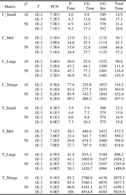
CONVERGENCE RESULTS OF PCG WITH ICDTPRECONDITIONER
Matrix
PCN Time P- CG Time CG Iter Total Time C_Small 10 1E-2 7.3E3 4.0 9.8 549 14.91E-3 7.2E3 4.2 12.0 546 17.3
50 1E-2 7.0E3 6.9 14.5 538 21.4 1E-3 7.1E3 8.2 17.3 542 26.6
C_Mid 10 1E-2 3.1E4 13.0 21.2 1132 36.7
1E-3 3.0E4 14.8 25.5 1114 42.3 50 1E-2 3.3E4 15.0 32.8 1168 49.8
1E-3 3.1E4 18.4 37.7 1132 57.2
C_Large 10 1E-2 5.6E4 40.6 52.9 1522 98.6 1E-3 5.5E4 43.2 64.1 1509 111.4
50 1E-2 5.3E4 45.1 77.2 1481 126.4
1E-3 5.3E4 46.8 91.5 1481 143.4
C_Xlarge 10 1E-2 8.3E4 77.6 229.8 1853 314.5 1E-3 8.1E4 83.4 277.5 1831 363.0 50 1E-2 8.2E4 85.9 342.7 1842 432.6 1E-3 8.2E4 89.3 406.2 1842 497.5
T_Small 10 1E-2 8.3E3 3.5 5.9 586 12.5 1E-3 8.1E3 4.6 7.2 579 13.8
50 1E-2 8.1E3 6.0 8.8 579 16.9
1E-3 8.0E3 7.3 10.4 575 19.8
T_Mid 10 1E-2 7.1E5 20.1 446.4 5422 472.5 1E-3 7.0E5 23.4 541.7 5383 569.2 50 1E-2 7.2E5 26.6 674.3 5460 704.0 1E-3 7.0E5 27.7 787.9 5383 818.6
T_Large 10 1E-2 6.5E5 41.8 835.3 5188 888.2 1E-3 6.3E5 43.1 1005.0 5107 1058.2 50 1E-2 6.3E5 55.3 1233.5 5107 1293.8
1E-3 6.0E5 58.1 1426.7 4984 1488.8
T_Xlarge 10 1E-2 9.1E5 82.2 2780.0 6138 2875.2 1E-3 8.9E5 85.4 3360.1 6070 3457.5 50 1E-2 9.2E5 96.0 4193.1 6172 4299.1 1E-3 9.0E5 108. 4914.8 6104 5025.6
It appears that the computation time taken by CG to solve the preconditioned system is far more dependent on the number of fixed fill-ins rather than on the drop tolerance since
IAENG International Journal of Applied Mathematics, 43:4, IJAM_43_4_05
[image:6.595.306.549.331.706.2]the fixed fill-in parameter determines the density of the preconditioner. The same comment can be given on the storage requirements of the preconditioner. However, in most cases, the drop tolerance has an obvious effect on improvement of the number of iterations of the CG method. According to these observations, the drop tolerance can be interpreted as a parameter responsible for the accuracy of the solution and the fixed fill-in number as a parameter to control the storage requirement and computational expense of the solver.
Factorized sparse approximate inverse (FSAI)
The results from applying PCG with FSAI preconditioner on our samples systems are presented in Table V. To build the preconditioner, a priori sparsity pattern needs be determined. In the reported results in Table V, two different sparsity patterns are considered. One is the same as the sparsity pattern of the coefficient matrix
A
and the other one is identical to that of the squared coefficient matrixA
2. Extensive experiments suggest that considering higher powers of matrixA
for this purpose is of no further improvement in the efficiency of the preconditioner since the cost of constructing the preconditioner grows significantly.TABLEV
CONVERGENCE RESULTS OF PCG WITH FSAIPRECONDITIONER
Matrix A
PRIORI PCN
P-Time CG Time
CG Iter
Total Time
C_Small A 1.1E+4 5.24 9.76 723 15.00
A2 9.5E+3 9.32 13.61 672 22.93
C_Mid A 8.6E+4 15.01 28.42 2023 43.43
A2 8.4E+4 24.72 42.13 1999 66.85
C_Large A 9.9E+4 41.46 56.64 2171 98.10 A2 9.5E+4 58.59 83.20 2126 141.79
C_Xlarge A 1.6E+5 82.43 256.76 2760 339.19 A2 1.2E+5 102.15 333.51 2390 435.66
T_Small A 2.5E+4 6.01 8.35 1090 14.36
A2 2.1E+4 12.89 11.48 999 24.37
T_Mid A 1.0E+6 20.30 426.09 6900 446.39
A2 9.8E+5 46.14 632.65 6830 678.79
T_Large A 9.6E+5 51.15 816.39 6760 867.54 A2
9.3E+5 83.82
1205.3 6654 1289.2
0
T_Xlarge A 2.3E+6 92.07 3554.5 10464 3646.5 A2 1.9E+6 145.41 4845.6 9510 4991.0
The results from Table V suggest that for all of the sample systems, although use of the sparsity pattern of
A
2 leads to a better conditioned matrix and reduces the number of CG iteration, the cost of construction of the preconditioner and the solution time of the PCG algorithm is much higher than the case of employing the sparsity patter ofA
. Moreover, compared to other preconditioning techniques reported so far, the efficiency of FSAI preconditioner in terms of total solution time of the PCG algorithm is quite comparable to ICDT and in most cases slightly better than FFIC. However, it is still outperformed by AJRIC with quite a considerable margin.Stabilized approximate inverse (SAINV(
))
Table VI presents the results of the employment of PCG method preconditioned with SANIV to solve the sample systems with two different values of drop tolerance
. Smaller values of the drop tolerance make the preconditioner construction time prohibitively longer. Note that as all sample systems are SPD, the SANIV preconditioner is computed without any breakdowns.TABLEVI
CONVERGENCE RESULTS OF PCG WITH SAINVPRECONDITIONER
Matrix
PCN P-Time CGTime CG Iter
Total Time C_Small 0.1 1.0E+4 5.31 9.18 680 14.49
0.01 9.6E+3 10.12 13.49 666 23.61
C_Mid 0.1 8.5E+4 14.30 27.85 1982 42.15
0.01 8.4E+4 20.72 41.52 1970 62.24
C_Large 0.1 9.7E+4 40.17 55.23 2117 95.40
0.01 9.5E+4 56.39 81.99 2095 138.38
C_Xlarge 0.1 1.7E+5 82.19 260.77 2803 342.96 0.01 1.4E+5 96.71 355.00 2544 451.71
T_Small 0.1 2.5E+4 6.49 8.24 1075 14.73
0.01 2.2E+4 10.75 11.59 1008 22.34
T_Mid 0.1 9.8E+5 21.62 415.65 6731 437.27 0.01 9.7E+5 39.79 620.33 6697 660.12
T_Large 0.1 9.7E+5 50.83 808.78 6697 859.61 0.01 9.3E+5 78.36 1187.8 6557 1266.1
T_Xlarge 0.1 2.1E+6 91.42 3347.3 9854 3438.7 0.01 1.8E+6 129.01 4648.4 9123 4777.4
Table VI reveals that while the time of constructing SAINV preconditioner is comparable to that of FSAI, the total time of the PCG algorithm is slightly shorter in the former case. Furthermore, selecting a smaller drop tolerance seems to increase the preconditioning time even higher with generally no significant achievement in terms of the CG time.
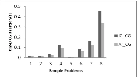
In addition, similar to FSAI, the SAINV preconditioner is also not as efficient as incomplete Cholesky variants at least in sequential computations. However, in parallel computations this comparison may lead to a totally different statement. Figure I compares the CPU time per PCG iteration with two major classes of preconditioners studied so far, i.e. incomplete Cholesky (IC-CG) and approximate inverse (AI-CG) techniques. As the purpose of such a comparison is to reveal the possible advantage of the approximate inverse preconditioners over incomplete Cholesky techniques in parallel environment, only the best performance results of each class of preconditioners for each problem are included in Figure I.
Figure I shows that the CG time per iteration is higher for CG preconditioned with incomplete Cholesky preconditioner. It is of no surprise as each iteration of an incomplete Cholesky preconditioned CG (IC-CG) includes one matrix-vector product and two triangular system solution while each iteration of an approximate inverse preconditioned CG (AI-CG) involves three matrix vector products.
IAENG International Journal of Applied Mathematics, 43:4, IJAM_43_4_05
FIGURE I:TIME PER CGITERATION WITH IC AND AIPRECONDITIONERS
According to Figure I, even in sequential environment, a matrix-vector product is computationally cheaper than a triangular system solution.
V.CONCLUSION AND FUTURE RESEARCH
In this paper we make an extensive numerical study of the preconditioning techniques for large sparse linear systems arising in the course of the interior point method applied to optimization problems in finite element limit analysis. We included in our study to most widely used classes of preconditioners, the incomplete Cholesky (IC) techniques and the approximate inverse (AI) methods. The systems arising in the specified application are usually highly ill-conditioned. As direct solvers can handle these systems efficiently in smaller sizes, we focus our attention to large sparse systems where the use of direct solvers is not practical due to prohibitive computational and memory costs.
Three variants of IC preconditioners and two variants of AI preconditioners which differ in the employed dropping rules were considered. In each case, a detailed parametric numerical study was conducted and the results were discussed and compared with other methods. The parametric study results can serve as a guide to choose the appropriate preconditioner with regards to the problem in hand and specific goals of the application.
Overall, the IC variants seem to be more efficient than the AI techniques in terms of their effect on the conditioning of the system and as a result the speed of the convergence of the method. Among various IC preconditioners, the Ajiz-Jennings’ robust incomplete Cholesky preconditioner (AJRIC) showed the best effect on the CG convergence, followed by the incomplete Cholesky preconditioner with double threshold (ICDT) and Incomplete Cholesky preconditioner with fixed fill-in (FFIC). Note that as for ICDT, the exact size of preconditioner is predictable in advance, in applications where this is desirable, ICDT could be an efficient choice.
The performances of the two AI preconditioners are closely comparable with a slight advantage toward the SAINV preconditioner. Although both AI variants are less effective compared to IC techniques, they possess a significant advantage over IC variants. In fact, even in sequential computations, the each iteration of PCG preconditioned with AI techniques is computationally cheaper than one obtained from IC preconditioning. Indeed, in a parallel computational
environment, the much more efficient parallelism characteristics of a matrix-vector product compared to a triangular system solution may compensate the more number of required CG iterations and, in total, outperform the incomplete Cholesky variants. This is an interesting direction for our future research.
REFERENCES
[1] M.A. Ajiz and A. Jennings, “A robust incomplete Choleski-conjugate gradient algorithm,” in International Journal of Numerical Methods in Engineering, vol. 20, 1984, pp. 949–966.
[2] E. D. Anderson, C. Roos, and T. Terlaky, “On implementing a primal-dual interior-point method for conic quadratic optimization,” in
Mathematical Programming, vol. 95, 2003, pp. 249–277.
[3] M.W. Benson, Iterative Solution of Large Scale Linear Systems, M.Sc. thesis, Lakehead University Press, 1973.
[4] M. Benzi, “Preconditioning techniques for large linear systems: A survey,” in Journal of Computational Physics, vol. 182, 2002, pp. 418–477.
[5] M. Benzi, J. K. Cullum, and M. Tuma, “Robust approximate inverse preconditioning for the conjugate gradient method,” in SIAM Journal
on Scientific Computing, vol. 22, 2000, pp. 1318–1332.
[6] M. Benzi, D. B. Szyld, and A. van Duin, “Orderings for incomplete factorization preconditioning of nonsymmetric problems,” in SIAM
Journal on Scientific Computing, vol. 20, 1999, pp. 1652–1670.
[7] M. Benzi and M. Tuma, “A comparative study of sparse approximate inverse preconditioners,” in Applied Numerical Mathematics, vol. 30, 1999, pp. 305-340.
[8] M. Benzi and M. Tuma, “A sparse approximate inverse preconditioner for nonsymmetric linear systems,” in SIAM Journal on Scientific Computing, vol. 19, 1998, pp. 968-994.
[9] M. Benzi and M. Tuma, “Orderings for factorized approximate inverse preconditioners,” in SIAM Journal of Scientific Computing, vol. 21, 2000, pp. 1851-1868.
[10] K. Chan, Matrix Preconditioning Techniques and Applications. Cambridge University Press, 2005.
[11] E. Chow, “A priori sparsity patterns for parallel sparse approximate inverse preconditioners,” in SIAM Journal on Scientific Computing, vol. 21, 2000, pp. 1804 - 1822.
[12] E. Chow and Y. Saad, “Parallel Approximate Inverse Preconditioners,”
in Proceedings of the Eight SIAM Conference on Parallel Processing
for Scientific Computing, SIAM , 1997, pp. 14-17.
[13] E. Cuthill, “Several strategies for reducing the bandwidth of matrices,” in Sparse Matrices and Their Applications, 1972, pp. 157-173. [14] M. R. Field, “Improving the Performance of Factorised Sparse
Approximate Inverse Preconditioner,” in Hitachi Dublin Laboratory
Technical Report HDL-TR-98-199, Dublin, Ireland, 1998.
[15] G. Gambolati, M. Ferronato, and C. Janna, “Preconditioners in computational Geomechanics: A survey,” in International Journal of
Numerical and Analytical Methods in Engineering, vol. 35, 2011, pp.
980–996.
[16] M. Grote and T. Huckle, “Parallel preconditioning with sparse approximate inverses,” in SIAM Journal on Scientific Computing, vol. 18, 1997, pp. 838-853.
[17] I. Hladik, M. B. Reed, and G. Swoboda, “Robust preconditioners for linear elasticity FEM analyses,” in International Journal of
Numerical Methods in Engineering, vol. 40, 1997, pp. 2109–2127.
[18] T. Huckle, “Factorized sparse approximate inverses for preconditioning,” in Journal of Supercomputing, vol. 25, 2003, pp. 109-117.
[19] M. T. Jones and P. E. Plassmann, “An improved incomplete Cholesky factorization,” in ACM Transactions on Mathematical Software, vol. 21, 1995, pp. 5–17.
[20] S. A. Kharchenko, L. Yu. Kolotilina, A. A. Nikishin and A. Yu. Yeremin, “A robust AINV-type method for constructing sparse approximate inverse preconditioners in factored form,” in Numerical Linear Algebra with Applications, vol. 8, 2001, pp. 165-179.
[21] L. Yu. Kolotilina, A. A. Nikishin and A. Yu. Yeremin, “Factorized sparse approximate inverse preconditionings. IV: Simple approaches to rising efficiency,” in Numerical Linear Algebra with Applications, vol. 6, 1999, pp. 515- 531.
IAENG International Journal of Applied Mathematics, 43:4, IJAM_43_4_05
[22] L. Yu. Kolotilina and A. Yu. Yeremin, “Factorized sparse approximate inverse preconditioning. I. Theory,” in SIAM Journal on Matrix Analysis and Application, vol. 14, 1993, pp. 45-58.
[23] O. Kardani, A. V. Lyamin and K. Krabbenhøft, “Preconditioned Conjugate Gradient for Large Sparse Systems Arising from Optimization Problems in Geomechanics,” in Proceedings of World
Congress on Engineering, 2013, pp. 216-221.
[24] K. Krabbenhøft and A. V. Lyamin, “Computational Cam clay plasticity using second-order cone programming,” in Computer Methods in
Applied Mechanics and Engineering, vol. 209-212, 2012, pp. 239 –
249.
[25] K. Krabbenhøft and A. V. Lyamin, and J. Huang, “Granular contact dynamics using mathematical programming methods,” in Computes and Geotechnics, vol. 43, 2012, pp. 165 – 176.
[26] K. Krabbenhøft and A. V. Lyamin, and S. W. Sloan, “Formulation and solution of some plasticity problems as conic programs,” in
International Journal of Solids and Structures, vol. 44, 2007, pp.
1533–1549.
[27] A. Li, “A new preconditioned AOR iterative method and comparison theorems for linear systems,” in IAENG International Journal of
Applied Mathematics, vol. 42, 2012, pp. 161–163.
[28] C.-J. Lin and J. J. More, “Incomplete Cholesky factorizations with limited memory,” in SIAM Journal on Scientific Computing, vol. 21, 1999, pp. 24–45.
[29] J.W.H. Liu, “Modification of the minimum degree algorithm by multiple elimination,” in ACM Transactions on Mathematical Software, vol. 11, 1985, pp. 141-153.
[30] T. A. Manteuffel, “An incomplete factorization technique for positive definite linear systems,” in Mathematics of Computation, vol. 34, 1980, pp. 473–497.
[31] J. A. Meijerink and H. A. van der Vorst, “An iterative solution method for linear systems of which the coefficient matrix is a symmetric M-matrix,” in Mathematics of Computation, vol. 31, 1977, pp. 148– 162
[32] M. U. Rehman, C. Vuik and G. Segal, “Preconditioners for steady Incompressible Navier-Stokes Problem,” in IAENG International Journal of Applied Mathematics, vol. 38, 2008, pp. 36-43.
[33] Y. Saad, “ILUT: A dual threshold incomplete LU factorization,” in
Numerical Linear Algebra with Applications, vol. 1, 1994, pp. 387–
402.
[34] Y. Saad, Iterative Methods for Sparse Linear Systems. SIAM, 2nd ed., 2003.
[35] T. Schlick, “Modified Cholesky factorizations for sparse preconditioners,” in SIAM Journal on Scientific Computing, vol. 14, 1993, pp. 424–445.
[36] R. B. Schnabel and E. Eskow, “A new modified Cholesky factorization,” in SIAM Journal on Scientific Computing, vol. 11, 1990, pp. 1136–1158.
[37] M. Tismenetsky, “A new preconditioning technique for solving large sparse linear systems,” in Linear Algebra with Applications, vol. 154– 156, 1991, pp. 331–353.
[38] S. J. Wright, Primal-Dual Interior-Point Methods. Philadelphia: SIAM, 1997.