ISSN Online: 2380-4335 ISSN Print: 2380-4327
DOI: 10.4236/jhepgc.2019.51001 Nov. 16, 2018 1 Journal of High Energy Physics, Gravitation and Cosmology
The Origin of the Color Charge into Quarks
Giovanni Guido
Department of Physics and Mathematics, High Scholl “C. Cavalleri” Parabiago, Milano, Italy
Abstract
Showing the origin of the mass in an additional coupling between field quan-tum oscillators, we formulate a hypothesis of a geometrical structure of the oscillators of “fields-particles”. In this way, we define the possible structure of quarks and hadrons (as the proton). This hypothesis is reasonable if one ad-mits field oscillators composed by sub-oscillators at semi-quantum (IQuO) and in which a degree of internal freedom is definable. Using the IQuO mod-el, we find the origin of the sign of electric charge in to particles and, in quarks, the isospin, the strangeness and colour charge. Finally, we formulate the structure of the gluons and the variation modality of the colour charge in quarks.
Keywords
Massive Coupling, “Aureus” Ratio, Geometrical Structure, IQuO, Semi-Quantum, Sub-Oscillator, Entangled Quantum Vacuum, Electric Charge, Isospin, Strangeness, Color, Gluon
1. Introduction
If we associate a wave behaviour to particles, you see the diffraction with elec-trons and photons, one can conjecture that “something” oscillates “inside” a particle. This conjecture is plausible even if the positivist literature has set aside it, because this is not directly verifiable with experiments. Instead, by this hypo-thesis, we could talk about internal “clock” with proper frequency (ω0). On this
basis, we could say that “the time is inside the particles”. In the same way, then we could discuss about Compton wavelength (c) or the spin of the particles, as
something of “space” “inside” these. All that pushes us to affirm that “the Space-Time is inside the particles”. Since we always speak of particles being in space-time (ST), you see the conception of frame reference, thus we can say that particles and Space-Time define reciprocally themselves and if particles are also
How to cite this paper: Guido, G. (2019) The Origin of the Color Charge into Quarks. Journal of High Energy Physics, Gravitation and Cosmology, 5, 1-34. https://doi.org/10.4236/jhepgc.2019.51001 Received: June 25, 2018
Accepted: November 13, 2018 Published: November 16, 2018 Copyright © 2019 by author and Scientific Research Publishing Inc. This work is licensed under the Creative Commons Attribution International License (CC BY 4.0).
http://creativecommons.org/licenses/by/4.0/
DOI: 10.4236/jhepgc.2019.51001 2 Journal of High Energy Physics, Gravitation and Cosmology
fields we can talk about Space-Time Field. From these ideas we can assume the permissible question of physically detect, even indirectly, the “internal” oscilla-tion. We, previously, have given a positive response to this question stating [1] [2] that the sign of electric charge is related to the phase rotation of an “intrinsic oscillation”, as well as the mass of the particles which is related [3] to “proper frequency” of this internal oscillation.
Thus, to talk about “internal” oscillation or Space-Time (ST) “inside” par-ticles, it is the same as talking about “internal structure” of a particle. However, if we assume (you see the relativity) that elementary particles (quarks and lep-tons) are simply points in ST, while in quantum theory are fields (Ψ), then we cannot consider them as composed by sub-particles, such as into nuclei or nucleons. However, if we want admit that inside particles there is an internal structure of “oscillators” and at the same time we want to be coherent with the relativity and Quantum Mechanics, then there is an only possible assertion: the idea of a structure of “coupled oscillators” which makes a particle as a unique and “not separable” object (see “elementary particle”). If, after, we recall that in quantum mechanics (QM) theory the fields are represented as a set of coupled quantum oscillators, then we can give “particles” of the field an internal struc-ture of coupled oscillators: this is the “hypothesis of strucstruc-ture” [1]. In this way we can think of quarks as geometric structures of coupled oscillators. However, speaking of structures of coupled oscillators does not imply that those structures are “rigid”: the same we could talk about components in movement (see the proton spin and of the quarks which compose them). Nevertheless, the “hypo-thesis of structure” is based on a previously hypo“hypo-thesis of quantum oscillators at semi-quanta called IQuO (acronym of Intrinsic Quantum Oscillator), you see ref. [1] [2]. In truth, we already discussed an internal geometric structure of the elementary particles and, exactly, we talked [3] [4] about quarks (u, d, s) and (c, b, t) as physical systems having a well-defined spatial geometric structure of coupled oscillators. Instead, in this paper we prefer to ignore previous works de-veloping these structures; then we will explore the road that starts from the hy-pothesis of structure and leads us to formulate a hyhy-pothesis of quantum oscilla-tors at semi-quanta called IQuO. We will then show the fundamental properties of the “IQuOs” and, through them, unveiling the meaning of fundamental phys-ical properties [5], such as the mass of the particles, the sign of electric charge, the Y hypercharge and the isospin in the quark [6]. Besides, after processing the quarks with the IQuO model (quantum oscillators defined with semi-quanta and sub-oscillators), we define the structure of the “gluons” [6] and we find the ori-gin of the “colour charge” and its structure in this model.
2. Hypothesis of Structure
2.1. Massive Coupling
DOI: 10.4236/jhepgc.2019.51001 3 Journal of High Energy Physics, Gravitation and Cosmology
which is given by the constant (c) in [p4= mc], (you see the relativity) and even
the concept of energy a rest. So we can speak of mass-energy like the energy of movement in time: all this is coherent to relativity. This uniform motion in time recalls once again the “clock” that exists inside every particle-object as a periodic “motion”. With proper frequency (ω0), which corresponds to [ω0 τ], where
(τ) is the proper time. The proper characteristic of a massive particle, associated with the proper time (τ) of an object, coincides with the proper mass (m0) of that
object. Then, discussing the mass or mass-energy of a particle, it is the same that to consider the time of the clock which is inside them [ωoτ mo]. Then,
based on QM [1]:
2
0 0
2
0 0
E mc m
c E
ω ω
=
⇒ =
=
(2.1)
If the frequency ω0 generates the proper time τ of a massive particle [τ =
/mc2], then for symmetry, there exists a wavelength
c that originates the
“proper space” of the particle [1]. Following De Broglie, we have:
0
0 0
0
2π c
p mc
p λ mc
=
⇒ = ≡
=
(2.2)
We assert that [c = /mc] (i.e., the Compton wavelength) defines the spatial
step of the proper ST of the massive particle. Now, combining the equation of the relativistic energy with the equations of De Broglie and Einstein, we have:
{
2 2 4 2 2 2 2 2 2}
0
E =m c +p c ⇔
ω
=ω
+k c(2.3)
The second equation is the dispersion relationship of waves, as described by the Klein-Gordon equation:
( )
( )
( )
2 2
2 2
0
2 2
, ,
,
x t x t
c x t
t x ω
∂ Ψ ∂ Ψ
= − Ψ
∂ ∂
(2.4)
As is well known, this equation describes the oscillations in a set of pendu-lums coupled through springs [3] and scalar fields associated with massive par-ticles with zero spin:
( )
( )
2( )
( )
2( )
2 2
2
2 2 2
, ,
, , ,
x t x t mc x t x t mc x t
x c t
∂ Ψ ∂ Ψ
− = Ψ ⇔ ∇ Ψ = Ψ
∂ ∂
(2.5)
We conjectured [3] that mass is a physical expression of the proper frequency (ωo) related to a particular elastic coupling, which is in addition to the one
al-ready existing between the oscillators of the massless scalar field (Ξ). This
“addi-tional coupling”, which produces the mass in a scalar field (Ξ), has been
re-ferred to as a “massive coupling” [7]. Then, we conjectured that the massive particle-field (Ξ) is originated by a “transversal coupling” (T0) between the
chains of oscillators of the scalar base field (Ξ). All that can be represented in
DOI: 10.4236/jhepgc.2019.51001 4 Journal of High Energy Physics, Gravitation and Cosmology Figure 1. The massive field as a lattice of “pendulums” with springs.
Therefore, a massive particle can be represented by lattice with transversal coupling on an Ξ-scalar field. The massive particles are so constructed by the
massive additional coupling which translates the “internal structure” of “coupled oscillators” into a geometric form.
2.2. Hypothesis of Structure
The massive particles are so originated by means of the massive additional coupling which builds the “internal structure” of “coupled oscillators” in geo-metric form.
A first geometric form we can find into proton considering an apparent coin-cidence between the Compton’s wavelength of Planck’s particle and the one of the proton. Following this coincidence and the “Hypothesis of Structure” [2], one can describe a proton as having a pentagonal geometric structure in which the constituent three quarks are coincident with three internal triangles (see the following Figure 2):
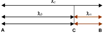
The vertices (A, B, C) are coincident with the three centres of diffusion in the interaction electron-proton. The structure is so because one high lights an “ au-rea” (golden) relation between the proton and Plank’s particle. Recall (see Fig-ure 3) the “aureus” (golden) segments:
By property of the “golden segment” one has:
2
γ β
γ α
φ φ
=
=
(2.6)
where (ϕ) is the “aureus” number. If we denote now with n(pl,p) the experimental
numerical ratio between the Compton’s wave length (pl) and (p),
experimen-tally it’s:
( )
(
)
(
(
)( )
)( )
8(
)( )
19, 27
2.176450 10
1.301220 10 1.672623 10
p pl
pl p
pl P
m n
m
−
−
= = = =
the power (10)(p) can be a representative scale factor (s). Remember that is:
(
) (
2)
2 1.618034 2.618034
DOI: 10.4236/jhepgc.2019.51001 5 Journal of High Energy Physics, Gravitation and Cosmology Figure 2. The geometric structure at quark of the proton.
Figure 3. “Aureus segments”.
We note that [n(pl,p)/(10)19] ~ [(φ)2/2] and [2n(pl,p) = (φ)2k].
Then by Equation (2.6), we note there is an “aurea” relation, less than a factor (10)p between the proton and the Planck particle. In universe where the
space-time is in expansion the spatial relations between some geometric struc-tures could “dilate” increasing in scale. So we assume that a particular spatial re-lation between particles could be invariant to any scale. Therefore, we could state that a proton is an “aurea” particle because it follows the relation (2.6a); in this way, we can consider the three quark which compose it as three “aureae” trian-gles [(u), (u), (d)]. The same, using the Hypothesis of Structure, a quark can be represented by three elastically coupled quantum oscillators. This hypothesis could allow us to represent [1] the (u, d) quarks as structures of coupled quan-tum oscillators, you see the Figure 2. The representative structure [1] is similar to one of three “spheres” placed at the vertices of an aureus triangle and con-nected by “springs” (“junction oscillators”). Nevertheless, these structure can be possible (see [2] [3]) only if we use particular quantum oscillators defined “IQuO” (acronym of Intrinsic Quantum Oscillator). Besides, we need adding that the three quantum oscillators need to constitute an individual physical ob-ject, i.e. a quark, and this says us that we cannot separately detect the IQuO, as shown in Figure 4.
DOI: 10.4236/jhepgc.2019.51001 6 Journal of High Energy Physics, Gravitation and Cosmology Figure 4. Quark sub-structure.
“structure” of components such as the “elastic” component and “absorptive” [3]. Therefore, this quantum oscillator with two components allows us to talk about a more elementary structure of it.
Another indication of a “composite structure” in quantum oscillator derives from its wave function (see Figure 5):
In fact, the quantum oscillator (with n the quantum number and n = 1) shows a wavefunction (Ψ) with a pair of peaks in the probability of detecting the energy quanta of the oscillation: we can describe therefore the quantum oscillator with two sub-units of oscillation or “sub-oscillators”. Into quantum oscillator with (n = 2) there are three peaks in wave function (Ψ) which denote three sub-oscillators (see the Figure 5).
Not only, but two components in an oscillator encourage us to believe that the energy of the “quanta” is distributed between the two oscillating components.
We think the presence of two components in an oscillator causes the splitting of its quanta of energy into two energetic components in each sub-oscillators: this introduces the idea of “semi-quanta” (or individually “semi-quantum”). A quantum oscillator with a sub-structure made of sub-units of oscillation, or “sub-oscillators” and “semi-quanta” is called “IQuO” [2].
3. The IQuO
3.1. The Quantum Oscillator at “
Semi-Quanta
”
We will explain the origin of the IQuO concept. The elastic couplings of field quantum oscillators transform each quantum field oscillator in a coupled oscil-lator. Therefore, each field oscillator acts as a “driven” oscillator, which, follow-ing oscillations theory, is described by two components: the absorptive ampli-tude (or “inertial” ampliampli-tude) and the elastic ampliampli-tude. By using ([2] [8]) oper-ators in phase plain (q, p) we derive the following equation:
( )
( )
( )
( ) ( )
ˆ ˆel 0 cos ˆabs 0 sin
q t =q ωt +q ωt
DOI: 10.4236/jhepgc.2019.51001 7 Journal of High Energy Physics, Gravitation and Cosmology Figure 5. Probability function of quantum oscillator.
Figure 6. Oscillator at two-components.
This hypothesis of field quantum oscillators may seem “extreme”; however, we observe that in the electromagnetic interactions a photon “forces” an elec-tron: at the point (P) of interaction the individual quantum oscillator of the electronic field is driven by the individual quantum oscillator of the electromag-netic field (photon). In this case the electronic field oscillator is described by two components. The same for the photon or electromagnetic field. All that leads us to build a two-component representation of the quantum oscillators of both in-teracting fields and free fields, when the latter represent particles which are structured by coupled oscillators (see i.e. the quark). Consequently, the two op-erators of oscillators annihilation (a) and creation (a+) which describe particles
have two components, an elastic component and the other inertial:
(
el, in)
;(
el, in)
a a a a+ a a+ +
→ →
In this way, the quantum oscillator with two components could have a “2-dim. representation”. This description cannot simply be a mere representa-tion because the existence of two components (el, in) in quantum operators (a,
a+) per se implies a 2-dimensional aspect. This concept introduces an internal
degree of freedom in the quantum oscillator. We could even say that this de-gree of freedom is highlighted in the interactions between particles (field coupl-ings): see the electric charge.
Only this quantum oscillator with two components allows us to talk about a more elementary structure of it. The quantum oscillator of the field no longer will be described by the pair of operators (a, a+) but by two pairs of operators
(
a ael, el+) (
, a ain, in+)
where the absorptive component becomes the inertial
DOI: 10.4236/jhepgc.2019.51001 8 Journal of High Energy Physics, Gravitation and Cosmology
( )
( )
( )
( )
( ) ( )( )
( ) ( ) ( )
π2
π2
ˆ ˆ e ˆ e
ˆ ˆ ˆ
ˆ ˆ ˆ ˆ ˆ e ˆ e
i t i t
t el in t elastic inertial
i t i t
t elastic inertial t el in
a a a
a a t a t
a a t a t a a a
ω ω
ω ω
− −
−
+ + + + + + −
= +
= +
⇔
= +
= +
(3.1)
This double structure of the operators (a, a+) splits the energy quanta of the
quantum oscillator, giving:
( ) ( ) ( )
( )
( )( )
( )(
2 1)
1(
2 1)
14 4
n n n n el n
el in
H U K U K
n ω n ω
= + = +
= + + +
(3.2)
A structure with two sub-oscillators involves that when the energy “quantum” is in one of two sub-oscillator the other sub-oscillator cannot be empty of energy but having the value of (ε = 1/2hν) defined “semi-quantum” (remember [ε(n=1) =
(1 + 1/2)hν)]). A structure with two components (elastic and “absorbing” or in-ertial) and two sub-oscillators would say that the “quantum” is composed by two (ε = 1/2hν) semi-quantum. Then we conjecture energy values of [(ε = 1/4hν)], indicated as “empty semi-quantum” and symbol (o), and another [ε = (1/4hν)], indicated as “full semi-quantum” and symbol (•). We will obtain the
probabilistic representation of the “semi-quantic” oscillator at a given instant (Figure 7).
An IQuO [εn = (n + 1/2)hν)] will be represented by empty semi-quantum
(ε(o) = 1/4hν), and full semi-quantum [ε(•) = (1/2hν)]; so [εn = (n + 1/2)hν) =
(n(1/2 + 1/2) + (1/4 + 1/4))hν]. We note that the semi-quantum flowing from a sub-oscillator to other.
We can represent the annihilation operator (a), and the creation operator (a+)
trough new operators built on the full semi-quantum (•) and empty semi-quantum
(o):
( )
( )
( )
( )
( )
( )
( )
( )
1 2
ˆ ˆ ˆ ˆ
ˆ ˆ o ˆ o ˆ
ˆ ˆ ˆ ˆ
ˆ o ˆ ˆ ˆ o
B -Matrix B -Matrix
el el in in el el in in el el in in el el in in
a a a a
a+ + a+ + a+ + a+ +
≡ • ≡ ≡ ≡ •
⇔
≡ ≡ • ≡ • ≡
(3.3)
The “commutation relation” of theoperators ((•), (o)) have been reported in
[2] and [3].
Here, there is a synthesis:
DOI: 10.4236/jhepgc.2019.51001 9 Journal of High Energy Physics, Gravitation and Cosmology
+
+
,o 0; ,o 0
o , 0; o , 0
,o ; o ,
2 2
,o ; o ,
2 2
el el in in el el in in
el in el in
in el in el
i i i i + + + + + + • = • = • = • = • = • = • = • = (3.4)
Then the Equation (3.1) in IQuO-representation will be:
( )
( )
( )
( )
( )
(
)
( )
(
(
)
)
( ) ( )
(
) ( )
(
(
)
)
( )
( ) ( )
(
( )
( )
)
(
( )
( )
)
+
ˆ ˆ
ˆ exp o exp π 2
ˆ
ˆ ˆ oˆ exp ˆ exp π 2
with
r el in
r
r r el in
el in el in
a t ir t i r t
a t t
a t a t ir t i r t
t a t a t a t a t a t a t
ω ω ω ω + + + ′ ′ ′ ′ + + + = • ′ + ′ −
Ψ ≡ =
= − ′ + • − ′ −
Ψ ≡ + = + + +
(3.5) where (r' = ±1) is connected to the direction of phase rotation.
For (r' = +1) the two equivalent representative ((2 rows) × (2 columns)) ma-trices (see Equation (3.1)) are:
[ ]
( )( )
( ) ( )( )
( )
( )( )
( )
( )( )( )
( )
( )( )( )
( )( )
( )( )
( )( )
( )( )
( )( )
( )( )
( )( )
( )( ) 2 2 2 2
1
+ +
2 2 2 2
( )
o o
o o
el cl in cl el cl in cl el cl in cl el cl in cl r
el cl in cl el cl in cl
el cl in cl el cl in cl
a a a a
a a a a
+ + + + × × ′=+ + + × × ≡
Ψ ≡
• • ≡ • • (3.6)
Omitting the time and the phase but highlighting the rotation direction (clockwise (cl)–anticlockwise (cl)). Besides, remember that inertial component is shifted to (π/2) by the elastic component. There are different configurations of IQuO in the pairs ((•), (o)) but all equivalents, as:
(
, +)
, o ,o(
)
(
o ,o ,+)
(
,)
in el el in in el el in
+ +
• • ⇔ • •
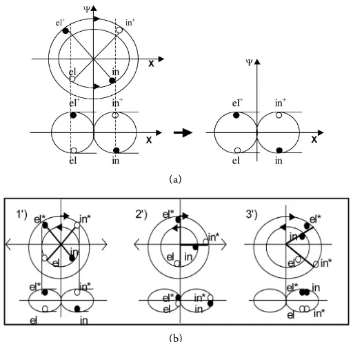
An IQuO (see Figure 8) can so have the following graphically representation into phase plain (q, ip), see [2] [3]:
Because two sub-oscillators compose the oscillator, going in the representa-tion of wave funcrepresenta-tion scalar (Ψ(x(t)) and highlighting the phase rotation, we will obtain a bi-dimensional representation of oscillators with
(
a ael, el+) (
, a ain, in+)
.It will be graphically (Figure 9(a)) and into instant: Note that the configuration is variable to the pass of time. The next configurations (Figure 9(b)) can be the following:
DOI: 10.4236/jhepgc.2019.51001 10 Journal of High Energy Physics, Gravitation and Cosmology (a)
[image:10.595.245.501.69.317.2](b)
Figure 9. (a) Graphic representation of an IQuO; (b) Next two configurations.
The 8-configuration will coincide with 1-configuration.
In the matrix representation, omitting the time and phase, this configuration is:
( )
(
(
5π5π44 7π74π)
4)
2 1 2 2
2 1
ˆ e ˆ e ˆ ˆ ˆ ˆ
ˆ
ˆ ˆ
ˆ ˆ
ˆ ˆ e
i i
el in el in el in i i
in in
el el
el in
o o o
o o
o
+ − + − + + + +
× ×
×
• + • + •
Ψ ≡ ≡ ≡
+ • •
+ •
(3.7)
where (oel, •in) is the couple with anti-clockwise phase rotation, while
(
o ,in+ •+el)
is the couple with clockwise phase rotation. Here we represent a matrix (2 × 1) as matrix (2 × 2) of components of Ψ. Note the energy exchange between full semi-quanta (•) with empty semi-quanta (o) (represented by [(•) (o)])
hap-pens in any point of axis x (see the equivalence between matrices in Equation (3.6). This because the operator
( )
+el →
•
creates a semi-quantum (•) on the
right, while
( )
oel → annihilates a semi-quantum (o) on the right: the same for( )
oin+ → and( )
•in →. Therefore, the two applications are equivalents becausethey indicate the propagation of a semi-quantum (•) the right.
Two IQuO (Ψ1, Ψ2) can be combined (Figure 10) in one zone of
superposi-tion (x):
Using the (⊕) combination operation [2]:
(
Ψ ⊕ Ψ = Ψ Ω Ψ1 2)
{
ˆ1 ˆ ˆ2}
(3.8)where the right side of Equation (3.8) contains the two representative matrices of the Ψ-IQuO and the Ω-operation defined as:
( )
(
)
( )
(
(
)
)
2 2
e 0
ˆ X ˆ ˆ X o
0 e
i i
ϕ
ϕ
ϕ − ∆
•⇔ ∆
×
Ω = ⋅ Σ ⋅ = ⋅ Σ • ⇔
DOI: 10.4236/jhepgc.2019.51001 11 Journal of High Energy Physics, Gravitation and Cosmology Figure 10. Two IQuO before of elastic coupling.
(X) is the operation representing the diagonal coupling of matrix elements
(Σ) is the operation representing the energy exchange between semi-quanta of different two IQuO, (exchange of full semi-quanta (•) of the first IQuO
with empty semi-quanta (o) of the other: [(•) (o)])
(φ) denotes the reduction of the wave function (Ψ) between phase shifts (∆φ)
(
)
( 0)e 0 ˆ 0 e 1 0 ˆ if 0 0 1 i i ϕ ϕ ϕ ϕ ϕ ϕ − ∆ ∆ ∆ = = ∆ = ⇒ = (3.10)
Then it is:
( ) ( )
( )
( )
( ) ( )
( ) ( )
( ) ( )
( ) ( )
( ) ( )
( )
( )
o
o o o
o o o o
el in el in el in el in
in el in
el el in el in
+ + + + + + + + • • • • ⊕ = + • • • • (3.11)
Note the X-operation is derived by associative property of addition (you see the Equation (3.5)):
(
)
{
( ) ( )
( ) ( )
}
( ) ( )
( ) ( )
{
}
( ) ( )
( ) ( )
{
}
( ) ( )
( )
( )
{
}
(
)
1 2 2 2 2 2
1 1
1 1
1 1 2 2
1 2 1 2 o o o o o o o o
el in el in
el in el in
el in el in
in el el in cl cl + + + + + + + +
Ψ ⊕ Ψ = • + + + •
+ • + + + • = • + + • + + + • + • +
= Φ + Φ
Graphically, the final result (Figure 11) is: With
( ) ( )
( )
( )
( ) ( )
( )
( )
( ) ( )
( ) ( )
( ) ( )
( ) ( )
+ + 1 2 1 21 2 2 2 1 2 2 1
+ +
el
1 2 1 2
1 2 2 2 1 2 2 1
o o o o o o o o in el in el cl el in el in
el in in
cl
el in el in
+ + × × + + × × • + •
Φ = ≡
• • + • + •
Φ = ≡
• • +
DOI: 10.4236/jhepgc.2019.51001 12 Journal of High Energy Physics, Gravitation and Cosmology Figure 11. Two IQuO whit phase rotation unidirectional.
where the numbers on the left indicate the two sub-oscillators. Note that the (Ψ1
⊕ Ψ2) coupling of two IQuO generates two particles-IQuO with opposite
direc-tion of the phase rotadirec-tion [(Φanti−cl) + (Φcl)]. Besides, note here the energy
ex-change [(•) (o)] between
(
ael+ ⇔ael) (
, ain+ ⇔ain)
not happens in anypoint (see Figure 11): the Ψ-IQuO is so essentially different from Φ-IQuO. We called Ψ-IQuO type as “Fermion” while Φ-IQuO as “Boson”. That is because we think that the IQuO are the fundamental quantum oscillators of all fields-particles.
3.2. The Electric Charge
An advantage in treating the field oscillators using the IQuO is that the “2-dimensional” representation (Figure 9) allows us” to distinguish the tion of rotation of the phase associated to oscillations having an only direc-tion of phase rotadirec-tion”. In fact, taking into account both the distribudirec-tion of semi-quanta inside the two sub-oscillators of an Φ-IQuO (I1) and both their
movement concerning the phase, another IQuO (I2) in coupling with first IQuO
(I1) it could detect the direction of rotation of the phase of (I1).
Note that IQuO I2(Ψ-type) could be the representative quantum of a particle
of interaction (i.e. photon). So, the direction of rotation of the phasedetermines a new degree of freedom in a quantum oscillator with semi-quanta. This degree of freedom admits two possibilities that would be interpreted as “the sign of the electric charge” of a particle. We conjecture that the IQuO [(Φanti−cl), (Φcl)] can
represent particles with opposite sign of electric charge [2]. This important result marks a turning point in the understanding of the physics of the interac-tions. We recall that the electric charge is in correlation with the generator of gauge transformation SU(2) which Pauli’s matrix is (σ3) [7] [8]; so, we can derive
the Q electric charge from the following equation, using the matrices (Φ) of the Equation (3.12):
( )
( )
( )
( )
3
3
ˆ d 1
ˆ d 1
cl cl cl
cl cl cl
Q V
Q V
σ
σ +
+
= Φ Φ = +
= Φ Φ = −
∫
∫
(3.13)commuta-DOI: 10.4236/jhepgc.2019.51001 13 Journal of High Energy Physics, Gravitation and Cosmology
tion relations with semi-quanta (see Equation (3.4) Appendix in [2]) it then fol-lows that: ( )
( )
(
)
(
( )
( ))
(
)
(
)
(
(
)
)
(
)
(
)
(
) (
)(
)
π2 π2
3 π 3π2 π 3π2
π2 π2 π 3π2 π 3π2
ˆ e ˆ ˆ e ˆ
ˆ ˆ ˆ d d
ˆ ˆ
ˆ e ˆ e e
ˆ e ˆ ˆ e ˆ ˆ e ˆ ˆ e ˆ e
ˆ ˆ ˆ
i i
el in el in
cl i i i i
el in el in
i i i i i i
el in el in el in el in
el in el
o o
Q V V
o o
o o o o
i o i
σ + + − + − − + − + − + + − + − + − + + • + • +
= Φ Φ =
+ − • + • = • + • + − + • + • = • − •
∫
∫
(
e πˆ3π2) (
ˆ ˆ e π2 ˆ e 3π2ˆ eπ)
ˆ ,ˆ ˆ ,ˆ ˆ ,ˆ ˆ ,ˆ 1
i i i i i
in in el in el el el in in el in el in
o o o
o o i o i o
− + − + − + + + + + • − • = • + • + • + • = − ( )
( )
(
)
(
( )
( ))
(
)
(
)
(
)(
) (
)(
)
π π2 π π2
3 π2 π2
π π2 π π2 π2 π2
ˆ ˆ
ˆ ˆ
( e e ) ( e e )
ˆ ˆ ˆ d d
ˆ e ˆ ˆ e ˆ
ˆ ˆ ˆ ˆ
ˆ e ˆ e e e e ˆ e ˆ
ˆ ˆ
ˆ ˆ
i i i i
el in el in
cl i i
el in el in
i i i i i i
el in el in el in el in el el el
o o
Q V V
o o
o o o o
o o σ − − + + + + + + + − − − + + + + − + + • + •
= Ψ Ψ =
• + • − +
= + • + • − • + • +
= • +
∫
∫
π2 π2
π2 π2
ˆ ˆ
ˆ ˆ
e e
ˆ ˆ ˆ ˆ e ˆ ˆ e ˆ ˆ
ˆ ˆ ˆ ˆ
ˆ , ˆ , ,ˆ ˆ , 1
i i
in in el in in
i i
el el el in in el in in el el in in in el in el
o o
o o o o
o o i o i o
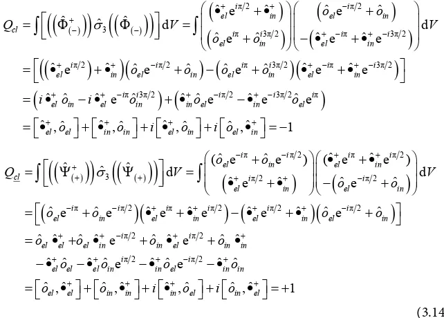
+ − + + + + + − + + + + + • + • + • − • − • − • − • = • + • + • + • = + (3.14) where [(Φ−) = (Φcl), (Φ+) = (Φcl)]and σ3 is a Pauli’s matrix.
Note, besides, the conjugation operation transforms the semi-quantum oper-ators:
( ) ( ) ( ) ( )
• → o , o → •
3.3. The IQuO
(n=0)The vacuum state of an “isolated” IQuO(n=0) will be graphically represented
(Figure 12):
Even here we can have some possible representations.
One of these (A-representation) can be the following (Figure 13): With representative matrices (2 × 1):
1 2 3 3
1 1 1 1
ˆ ˆ
o o
ˆ ˆ
o , o ; ,
ˆ ˆ
o o oˆ oˆ
a b
In El In El
El G In G El G In G
+ +
+ +
(3.15)
[image:13.595.213.534.107.337.2]The conjugate representation (Figure 14) is: And the conjugate matrices:
DOI: 10.4236/jhepgc.2019.51001 14 Journal of High Energy Physics, Gravitation and Cosmology Figure 13. Possible A-representations of isolated sub-oscillator.
Figure 14. Conjugate A-representation of sub-oscillator.
3 3
1 2
ˆ ˆ
ˆ ˆ o o
o o
, ; ,
ˆ ˆ
ˆ ˆ o o
o o
a b
El In
El In
In El
In G El G G G
+ + + +
(3.16)
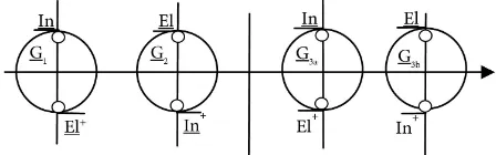
We note that the two possibilities (G3a, G3b) are indeed one only possibility
because (G3a)+ = (G3b); then we admit one only possibility → (G3)A. We obtain:
(Figure 15)
With representative matrices:
1 2 3
3
1 2
1 1 1
1
1 1
ˆo
ˆ ˆ
o , o ,
ˆ ˆ
o o ˆo
ˆ
ˆ ˆ o
o o
, ,
ˆ
ˆ ˆ o
o o
In
In El
El G In G El G
El
El In
In
In G El G G
+ + + + + + (3.17)
The other possible representation (B-representation) is: (Figure 16) Which becomes: (Figure 17)
Nevertheless note [(G1)B−rep = (G2)A−rep; (G2)B−rep = (G1)A−rep]; it follows that for
[(G1), (G2)] the two representation are coincident, instead for (G3) it’s not
possi-ble: [(G3)A−rep≠ (G3)B−rep].
Two are the possibilities: the combinations [Gi3, Gi3]B−rep have not physical
meaning or we can admit a combination between [(G3)A−rep, (G3)B−rep]. We opt
for the second:
3 3 3 3 3 3 1 1 1 1
ˆ ˆ ˆ
o ˆo o o
ˆ
ˆ o ˆ ˆ
o o o
ˆo ˆo oˆ oˆ
ˆ
ˆ o
o oˆ oˆ
B A
B A
In In In In
El El
El G G El G
El El El El
In
In G G In In G
+ + + + + + + + + ⊕ + ≡ + ⊕ + (3.17a)
Note that the two possibilities [(G3)A−rep, (G3)B−rep] indicates always a different
DOI: 10.4236/jhepgc.2019.51001 15 Journal of High Energy Physics, Gravitation and Cosmology Figure 15. The unique possible combination for (G1, G2, G3A).
Figure 16. B-representation.
Figure 17. B-representation of base.
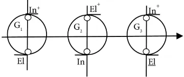
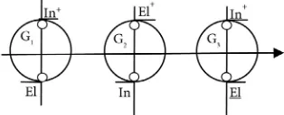
or a combination of them (see the 3.17a). We’ll have the following representa-tion (Figure 18 and Figure 19):
We call the IQuO(n=0) as IQuO-0.
If we call the three internal degrees of freedom (Gi) as “color charge” then we
will define three colors [(G1≡ GRed), (G2≡GBlu), (G3≡ GYellow] with
representa-tions (Figure 20): And matrices
ˆ ˆ
o 0 o
ˆ ˆ
o o 0
ˆ ˆ
o o 0
ˆ ˆ
o 0 o
ˆ ˆ
o 0 o
ˆ ˆ
o o 0
In In
R
El R El R
El El
B
In B In B
In In
Y
El Y El Y
G
G
G
+ +
+ +
+ +
= ≡
= ≡
= ≡
(3.18)
3.4. The Electric Charge of Quarks
As we know the abstract space to describe the hadrons, requires the transforma-tion group SU(3). The generators of the group are the Gell-Mann matrices asso-ciated with three variables (Y, T3, Q). Remember that the multiplets existing in
the hadrons are described by three physical quantities: hypercharge (Y), the isospin (T3) and the electrical charge Q. We focus on the matrices λ3 and λ8, two
DOI: 10.4236/jhepgc.2019.51001 16 Journal of High Energy Physics, Gravitation and Cosmology Figure 18. The unique possible combination.
Figure 19. Conjugate representation of sub-oscillator.
Figure 20. Sub-oscillators with color.
3 8
1 0 0 1 0 0
1
ˆ 0 1 0 ; ˆ 0 1 0
3
0 0 0 0 0 2
λ λ
= − =
−
(3.19)
The λ3 matrix is the projection in SU(3) of Pauli’s matrix σ3, giving [2] the
values of Q in the representation of the eigenvectors basic (Φ+, Φ−). We recall (in
Gell-Mann theory) the correlation between Y and the matrix λ8:
8
1 0 0
1 ˆ 1
ˆ ˆ 0 1 0
3
3 0 0 2
Y λ Y
= ⇒ =
−
(3.20)
Giving the correlation between the charge Q and the isospin T3 and Y, we can
consider the matrix product [3 = (λ3)(Y)]
( )
( )
3 3
1 0 0 1 0 0 1
ˆ ˆ ˆ 0 1 0 0 1 0
3
0 0 0 0 0 2
1 0 0 1 3 0 0
1 0 1 0 0 1 3 0
3
0 0 0 0 0 0
Y
λ
= = −
−
= − = −
[image:16.595.285.459.271.417.2]DOI: 10.4236/jhepgc.2019.51001 17 Journal of High Energy Physics, Gravitation and Cosmology
In conclusion, the matrix (3) can tell what values are allowed to charge Q of a
quark.
Then we think the IQuO of quark is expressed by matrix (1 × 3). In fact, if we recall the form of the wave function (see Figure 5) of the quantum oscillator with (n = 2) where there are three probability peak, then we can think that a IQuOI(n=2) is made with three sub-oscillators. The superposition of two IQuO
I(n=1) or (I1(n=1)⊕I2(n=1)) builds an IQuO(n=2) with three sub-oscillator but with the
pairs [(•, o)1; ((•, o)2, (•, o))2; (•, o)3] where the index numbers indicate the
sub-oscillators. This coupling can produce: 1) Two different IQuO (see the Equation (3.11)) 2) An excited and unstable IQuO I(n=2)
The b-possibility could be unstable because the central sub-oscillator is over-populated in full semi-quanta (•). For have a stable IQuO in eigenstate I(n=2) we
need of overlapping an IQuOI(n=1) with I(n=0): but this is possible only if we use
quantum oscillators at semi-quanta and if the I(n=0) is excited (I(n=0*)), that is we
have an IQuOI(n=0) composed by the pair [(•, o)]. Note that to make couplings
between sub-oscillators of two IQuO different it needs the exchange a full semi-quantum between the two respective component oscillators: this is allowed by a reciprocal intersection between the two IQuO (see Figure 21):
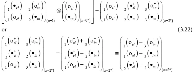
So, we need to define an operation (⊗) stating an appropriate combination of
two matrices [(2 × 2) and (2 × 1)] generating one matrix (2 × 3). Using the ma-trix representation:
( ) ( )
( ) ( )
( )( )
( )
( )( )
( )
( )
( )
( )
( )
( )( ) ( )
( )
( )
( ) ( )
( )( ) ( )
( )
( )
( ) ( )
( ) 31 2 1 2
1 2 1 0* 1 2 3 2*
1 3 1 3 1
2 2
2 2
1 3 1 3
2* 2*
o
o o o
o o
or
o o o o o
o o
in
el in el el el
el in n in n el in in n
el in el in el
el in el in
el in el in
n n + + + + + + = = = + + + + + + = = • • ⊗ = • • • • + • • = • + • ≡ • + •
( ) ( )
( ) ( )
( )
( )
( ) 3 1 3 2 2 2* o o in el in el in n + + + = + + • • + • (3.22)where the index numbers indicate the sub-oscillators and where it is happened the change (• o) between different sub-oscillators. The ⊗-operation thus
[image:17.595.228.542.405.522.2]im-plies an “elastic” attachment of sub-oscillators: [(2)sub + 1sub = 3sub].
DOI: 10.4236/jhepgc.2019.51001 18 Journal of High Energy Physics, Gravitation and Cosmology
Note that the result of the overlap between IQuO depends on the coupling of different modes.
We can reorganize the semi-quanta and elements of matrix obtaining the fol-lowing (3 × 1) column matrix (whit the relative phases):
( )
( )
(
)
(
)
(
)
ˆˆ e e
ˆ
ˆ e e
ˆ e ˆ e
i i el in i i el in cl i i el in c o o o ρ ρ σ σ α α − − ° + − + − ° + − − ° + •
Φ = + •
• +
(3.23)
[image:18.595.216.539.256.345.2]where index c indicates the couple of semi-quanta of the central sub-oscillator in Figure 21 and where [(α˚ = α + π/2), (ρ˚ = ρ − π/2), (σ˚ = σ ± π/2)].
It follows [2] the electric charge of IQuO(n=2*):
( )
( )
( )
( )
(
)
(
)
(
)
(
)
(
)
(
)
3 ˆ ˆˆ e e 1 3 0 0 ˆ e e
1
ˆ ˆ
ˆ e e 0 1 3 0 ˆ e e
3
0 0 0
ˆ e ˆ e ˆ e ˆ e
cl cl cl
i i i i
el in el in
i i i i
el in el in
i i i i
el in el in
c c
Q
o o
o o
o o
ρ ρ ρ ρ
σ σ σ σ
α α α α
+
+ − + − ° − − °
− − ° + − + − °
− + − ° + − − °
= Φ Φ
+ • + • = + • − + • = − • + • + (3.24)
Considering the ((Δ3)) as difference matrix of the matrices [((3)), ((Q) ≡λ3)]
we obtain the other value (Q = −2/3).
Note that the last pair of operators
(
o ,el+ •in c)
is not involved in the calculusof the electric charge; this meaning that there is inside the quark another freedom degree.
As mentioned this couple is representing the color charge.
3.5. The Isospin
Taking up the idea of “internal” rotation of the phase [2] into IQuO, further “internal” rotations into a “composed” particle (as is a hadron) could be identi-fied [1].
Remembering the electric charge connected to rotation of the phase of an IQuO (as “internal” rotation), we could connect the isospin (since it has similar structure to that of the “spin”) to an “internal rotation” of “something” existing “inside” the hadrons.
DOI: 10.4236/jhepgc.2019.51001 19 Journal of High Energy Physics, Gravitation and Cosmology
Remember that matrix σ3 is also used to represent the projection (T3) of
isos-pin T in the complex space Q (2). In fact, it’s:
3 3
1 0 0
1 ˆ 1
ˆ 0 1 0
2 2 0 0 0
T λ
= = −
(3.25)
This formal analogy between σi e (Ti), as between σ3 and (T3), cannot be
ran-dom.
Also, note that the formal analogy between (T3) and the spin of a composite
particle induces assign a value of (T3) also to the quarks.
It is recalled in fact the summative character of the isospin, then it follows that the isospin of a hadron is the sum of the values of isospin assigned to each indi-vidual quark.
Furthermore, the correlation between T3 and Q, leads us to admit the
exis-tence of a correlation between the direction of rotation of the phase and the one of the isospin current.
This clearly happens in individual quarks, because there are the following as-sociations:
1) Quark (u): Q (>0) ←→ (T3)' = (+1/2)
2) Quark (d): Q (<0) ←→ (T3)' = (−1/2)
Note that Q and T3 have the same sign
Thus, ultimately, we can assign three intrinsic “rotations” to IQuO-quark: 1) Internal phase rotation (Q sign)
2) Internal Isospin rotation (T3 sign)
3) External Spatial rotation of spin (σ sign)
This may seem at odds with the “spatially local” aspect assigned to the ele-mentary particle (like quarks and leptons), in perfect agreement with the relati-vistic quantum theory. However, considering what already talked about the rota-tions inside to hadron and taking into account the phenomenology of the inte-ractions between hadron, it can become acceptable assume the following hypo-thesis of Structure: even if an elementary particle proves to be a “local unit” in space for an external observer, it may instead show the existence of an “internal” space because described by variations of physical quantities that can be identi-fied as “internal” rotations showing an “internal structure” of couplings of IQuO.
If the isospin (Th) assigned to a hadron identifies an internal current
(semi-quanta current or “gluonic” current) then the isospin (Tq) assigned to a
quark identically detects a semi-quanta current that identify a “path” between elementary “internal points of oscillation”, though always considering a quark as an “oscillating” unique physical system.
DOI: 10.4236/jhepgc.2019.51001 20 Journal of High Energy Physics, Gravitation and Cosmology
being introduced to differentiate the hadron multiplets, is assigned to an indi-vidual quark, reinforcing the idea of its sub-structure related to different confi-gurations of coupling of sub-IQuO that make it.
3.6. The Hypercharge
Y
Another support for this hypothesis of Structure is identifiable in the correla-tions between the “internal” rotacorrela-tions (those of phase and isospin) during the hadron interactions (you see Clebsch-Gordon coefficients).
It was noted that Q and T3 have the same algebraic sign; this implies that the
isospin current between “Sub-IQuO” constituents of a quark follows the same “direction” of rotation of the phase of each Sub-IQuO. It’s evident that the structure of sub-IQuO (you see Y hypercharge) has to be compatible with the correlation (Q ←→ T3). It follows that has to exist a connection (Q ←→ T3 ←→
Y).
The relation of Gell-Mann expresses this connection: [Y = 2(Q − T3)]
The correlation (Q ←→ T3 ←→ Y) made manifest both in the correlation
be-tween the matrices λ3 e λ8, as we shall see later, both in the combination of the
respective generators during interactions.
Underlining the correlation of the sign of Q (direction of phase rotation) with the sign of T (direction of current rotation) and with a value of Y (structure by couplings), one derives that the electric charge values are connected with the structure of quarks. It’s evident that this connection determines in hadron inte-ractions the various probabilities of the combination of isospin couplings as the probabilities of the electric charge values of the quarks. This also suggests that the non-integer value of the charge of a quark is an expression of probabilistic aspects associated with the structure of couplings of the sub-IQuO which com-pose the quark. If the direction of phase rotation of a particle-IQuO gives to us the sign of the electric charge, its value can instead be placed in relation with the probability that a photon detects the quanta of the charged particle which has a particular structure of sub-IQuO. If into electron this probability has a value equal to one, the probability in quarks has not an integer value be-cause the triangular structure of a quark has a number of quanta minor that the number of sides. If inside a quark there are more sub-IQuO, the photon in coupling with one of sub-IQuO components cannot find the representative quantum of the quark. For the definition of statistical probability, if a quark may be no seen by a single photon, then it will be not seen by an infinite number of photons. How to say that a quark would be invisible to single photon.
However, if the single quark cannot be seen, a hadron composed by more quarks can be detected only if the sum of the probability of finding the quantum has a value of a unit or the sum of the electric charges of the quarks of a hadron reaches the value of a unit. This is because two or three quarks bound to become a single unit (or a single center diffuser) for couplings with photons.
DOI: 10.4236/jhepgc.2019.51001 21 Journal of High Energy Physics, Gravitation and Cosmology
also be found in the Gell-Mann matrix λ8, which is an expression of the
connec-tion (Q ←→ Y). In fact, (see the equation 3.19) it is no random coincidence that the matrix λ8 precisely commutes with the λ3 (you see σ3). In [1] so note that the
eigenvalues of Y are related to the values of electric charge Q. Obviously, every-thing is perfectly in accord with the relation: [Y = 2(Q − T3)]).
Therefore, we think that the quark is given by one “triangular” structure of three “sub-IQuO” (see IQuO-vertices) coupled to each other through IQuO chains (sides) in which flows a current of semi-quanta. The variable descriptive of the semi-quanta current is the Isospin (T) whose projection (T3) is connected
to the rotation direction of the current, we have the following correspondence:
Clockwise T3 = −1/2
Anticlockwise T3 = +1/2
The variable descriptive of the phase rotation in IQuO-vertices is electric charge Q:
Clockwise (−Q) Anticlockwise (+Q)
By triangular structure of the couplings, it follows that the direction of rota-tion of the semi-quanta current along the sides shall be concordant with the di-rection of rotation of the phase of IQuO-vertices. This expresses the correlation (Q T3). Also to its structure, it shall be associated with descriptive variable
that we believe it is the Y (hypercharge). It is evident that the probability of finding the quantum of a particle inside of a structure depends on this latter. As the value of the electric charge Q has been associated with the probability of de-tecting the representative quantum of the quark, it follows the (QY)
correla-tion. The correlation (QYT3) is now: Clockwise Q = [(−1/3, −2/3)]
Anticlockwise Q [(+1/3, +2/3)]
We ask in what way the Y is related to the structure. A triangular structure of IQuO-V coupled suggests that get involved more chains of IQuO and therefore it should exist the possibility to realize a coupling “transverse” between separate chains. Chains involved in the triangular closure defining a quark can be in a number of two or three at the most (you see the Figure 7 and Figure 8).
For everything that we affirmed up to now, we can say that the hypercharge
Y is the indicating physical variable the triangular structure of coupling of Sub-IQuO vertices to which we associate the value 1/3 as to say that there is one particle-quantum on three vertices. Also, noting that a triangle in the mirror (P) undergoes inversion right - left, we assign the value of the hypercharge Y = −1/3 to the antimatter. We note that the direction of rotation of any rotating object reflected in the mirror is reversed, thus both the isospin both the electrical charge changing the sign: [(±T3 → T3)]. It obvious then that you must also have
a reversal of the value of hypercharge (±Y → Y). We have thus explained the physical meaning about what we describe with electric charge Q, with isospin T
DOI: 10.4236/jhepgc.2019.51001 22 Journal of High Energy Physics, Gravitation and Cosmology
4. The Structure of Coupled Oscillators
4.1. The Coupling of Chains
If to an only oscillator (quantum and classic) we assign an elastic component (see ael in quantum oscillator) which represents the elastic tension (k) acting on
the “mass” (M) of oscillator (see ain), to the chain of coupled oscillators we
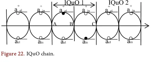
as-sign [1] the same elastic tension (k) between oscillators (see Figure 1). The same aspect is in the two sub-oscillators which component the IQuO. In summary: so as two sub-oscillators couple for making an only IQuO, then it is possible that more IQuO couple for making up a “chain” of coupled quantum oscillators. To chain (see Figure 1) is assigned an elastic tension T: [k∆l]. We think that can be possible the following representation of chain (Figure 22):
Note (see Figure 8 and Figure 9(a)) that the semi-quanta oscillate (•) inside
each IQuO: the couple ((•), (•)) would oscillate always only between the points
(A, C) in IQuO 1. Nevertheless, it is necessary even that the couple ((•), (•))
propagates along the X-axis: the propagation from IQuO-1 to the next (IQuO-2) needs so to oscillate with variable frequency (ω). To have both propagation and oscillation of couple ((•), (•)) it needs a superposition with another chain, but
shifted (of π/2): this could allow an oscillation of the full semi-quantum couple ((•), (•)) inside a sub-oscillator of IQuO and after the propagation along axis X.
In first we report the figure of two IQuO (you see Figure 23) in a particular overlap:
We note that two IQuO overlap and sharing the sub-oscillator central. Two IQuO can exchange energy only in the point C of the central sub-oscillator. The operation of superposition is indicated by (⊕): (⊕) is the overlap of two IQuO
involving an only sub-oscillator of two IQuO (see Figure 23).
We note the exchange [(ain)(•) → (Ain)(o)] happens in point C of the
configu-ration; these exchanges make oscillate the couple ((•), (•)) inside central
oscilla-tor just once because after it happens the passing to first sub-oscillaoscilla-tor of the 2-IQuO.
In this way, the quantum ((•), (•)) can propagate with oscillations along the
chain and so to constitute a “field chain”. It follows any field can be represented by a set of “field chains”. In the case of closed chains (see the sides of a triangular structure) then the superposition of two chains in each side is the fundamental condition for having the oscillating propagation of couple ((•), (•)) along the
[image:22.595.249.524.629.732.2]sides. It is evident that this determines even the “isospincurrent” inside the tri-angular structure of quark.
![Figure 21 where index c indicates the couple of semi-quanta of the central sub-oscillator in and where [(α˚ = α + π/2), (ρ˚ = ρ − π/2), (σ˚ = σ ± π/2)]](https://thumb-us.123doks.com/thumbv2/123dok_us/9251452.413531/18.595.216.539.256.345/figure-index-indicates-couple-semi-quanta-central-oscillator.webp)