The Volatilization of Pollutants from Soil and Groundwater: Its Importance in Assessing Risk for Human Health for a Real Contaminated Site

The Volatilization of Pollutants from Soil and

Groundwater: Its Importance in Assessing Risk for

Human Health for a Real Contaminated Site

Pamela Morra, Laura Leonardelli, Gigliola Spadoni

Department of Chemical, Mining & Environmental Engineering, Alma Mater Studiorum, University of Bologna, Bologna, Italy. Email: pamela.morra@unibo.it

Received July 25th_{, 2011; revised August 29}th_{, 2011; accepted October 4}th_{, 2011.}

ABSTRACT

Pollution of different elements (air, water, soil and subsoil) resulting both from accidental events and from ordinary industrial and civil activities causes negative effects on the human health and on the environment. The present paper examines the analysis of a contaminated site, focusing the attention on the negative effects for receptors exposed to soil and groundwater contamination caused by industrial activities. The case study investigated is a contaminated area lo- cated in the industrial district of Trento North once occupied by the Italian Carbochimica plant. Pollution in that area is mainly due to contamination of soil and groundwater with polycyclic aromatic hydrocarbons. The methodology ap- plied is the risk evaluation for human health, in terms of individual cancer risk and hazard index. In particular the at- tention has been focused on a specific migration way: if pollutants in the soil or in the groundwater undergo a phase change, they spread and get to the soil surface, causing a dispersion of vapors in the atmosphere. In this case risk as- sessment calls for the evaluation of volatilization factor. Among the different models dealing with the estimation of volatilization factor, those mostly known and used in the national and international field of Human Health Risk As- sessment were chosen: Jury’s and Farmer’s models. A sensitivity analysis of models was performed, in order to identify the most significant parameters to estimate the volatilization factors among the wide range of input parameters for the application of models. Performing an accurate selection and data processing of the contaminated site, models for the volatilization factors calculation are applied, thus evaluating air concentrations and Human Health Risk. The analysis of the resulting estimates is an excellent aid to draw interesting conclusions and to verify if the soil and groundwater pollutants volatilization affects the human health considerably.

Keywords:Human Health Risk Assessment, Volatilization Models, Soil Contamination, Groundwater Contamination,

Cancer Risk, Hazard Index

1. Introduction

Pollution of different elements (air, water, soil and sub- soil) resulting both from accidental events and from daily industrial and civil activities, implies effects on the hu- man health and on the environment. Through the appli- cation of the Human Health Risk Assessment methodo- logy in a specific contaminated site, it is possible to eva- luate the magnitude and probability of negative effects posed to human beings caused by exposure to contami- nation in various media [1]. The consolidated procedure concerning the risk analysis applies the RBCA approach [2], which refers to a step method based on three levels of assessment. In the following we refer to a tier 2 risk assessment, involving site-specific data collection and

analytical modeling of the fate and transport of contami- nants across the environmental media involved (in par- ticular unsaturated soil, groundwater and outdoor air).

final individual cancer risk and hazard index for a recep- tors group.

In the present paper the attention has been focused on the pathway of volatilization of hazardous vapors coming from contaminated soil and groundwater into open air and consequent exposure of receptors to COCs. The aims of this study are to: 1) identify the parameters that more affect the estimate of the volatilization factors and their uncertainty, 2) evaluate the importance of volatilization of pollutants from soil and groundwater in the risk as- sessment for human health through the application of the models to a real contaminated site case-study.

In order to reach the first objective, a selection of sim- ple and diffusely used models for the estimation of vola- tilization factor in risk analysis was performed thus op- erating a sensitivity analysis on input parameters for the application of models; the second objective has been approached through the investigation of a case-study concerning a contaminated area located in northern Italy, where contamination of soil and groundwater is mainly due to polycyclic aromatic hydrocarbons deriving from the productive cycles in remote industrial activities.

2. Vapors Migration modeling

In the assessment of human health risk, the estimation of transport factors is necessary, thus considering the mi- gration of pollutants from the contamination source to the targets. When the volatilization is regarded, the trans- port factor is called volatilization factor (VF) and con- siders the attenuation phenomena occurring during mi-

gration. VF represents the ratio between the pollutants

concentration in the exposure site (cpoe, expressed for

example in mg/m3_{) and the concentration at the contami-}

nation source (cs expressed for example in mg/kg), as

resulting from soil samples or calculated applying mo- dels:

poe s

c VF c (1)

Detailed models of contaminant transport in soil and groundwater include processes such as diffusion, disper- sion and convection phenomena for each of the phases present in the soil. Obviously, such models include a large number of contaminated site parameters and soil- specific parameters that are often not available or not very accurate. Therefore, in most volatilization pheno- mena estimates, predictive models are simplified in order to allow the application of models even in situations where a few site specific parameters are available [4]. For every soil layer a different volatilization factor is

identified: VFss (volatilization of outdoor vapors from

surface soil), VFds (volatilization factor of outdoor vapors

from deep soil), VFgw (volatilization factor of outdoor

vapors from groundwater). These factors are used to es-timate outdoor air concentration of volatiles by using the known chemical concentration in the groundwater and soil.

Among the volatilization models from subsurface sou- rces into outdoor air available in literature, two models were selected, widely applied in the Risk Assessment for Human Health and Environment and suggested by EPA [1,5,6], ISPRA [7] and ASTM standard [2,8].

In detail the volatilization models selected are:

- Jury’s model [9,10], assuming a contamination source with semi-infinite dimensions and time-varying concen- trations (estimation of VFss,J1 and VFss,J2 for surface soil

and VFds,J for deep soil),

- Farmer’s model [11], with steady-state assumption (estimation of VFss,F for surface soil, VFds,F1, VFds,F2 for

deep soil and VFgw for groundwater).

These models make the following common assump- tions when calculating volatilization factors: uniform and isotropic soil (fissuring-porous soil is not considered); the chemicals do not biodegrade in soil, in water solu- tions or in vapor phase; no transport within water, no absorption or production of the gases; the partitioning between the chemicals in the groundwater/soil matrix and vapors is linear; chemical losses by biodegradation do not occur between the groundwater/soil and the sur- face; for outdoor emissions, steady-state atmospheric dis- persion of vapors occurs within the breathing zone.

The calculation of VF, hence the concentration of vo- latiles outdoors, is based on the movement of volatiles from the soil and groundwater up through the capillary zone, through the unsaturated zone, and emission into the breathing zone in outdoor air (Figure 1).

The models relationships are derived from simple one- dimensional or integral mass balances, based on the dif-

Groundwater Contaminated

groundwater

Capillary zone Deep soil

Surface soil

Vadose zone Contaminated

sub-soil

Contaminated surface-soil Air Mixing Height

Wind direction

ferent hypothesis of the considered volatilization models. In particular VFss,J1 derives from Jury’s model, based

on the one-dimensional application of Fick’s laws con- sidering the following assumptions and conditions: ab- sence of boundary layer at the interface soil-air, thus assuming a perfect mixing situation in air; no water flow is considered through the soil (the pollutant’s loss due to its transport into the groundwater is thus not considered and lisciviation is therefore considered apart from vola- tilization); the soil contaminated column of semi-infinite depth has homogeneous physical characteristics; finally a boundary condition considers that the soil concentration at the ground level must be zero.

It’s worth noting that the condition of equilibrium par- titioning is very rarely accomplished in the subsurface, therefore calculated soil vapor values from soil-phase data may clearly overestimate or underestimate actual soil vapor concentration.

VFss,J2 and VFds,J are the upper limit of Jury’s model

and as a result are a conservative evaluation. Briefly, they consider a mass balance in which the total value of mass that can enter into the mixing volume (correspond- ing to the total mass of pollutants in the surface soil) is equal to the mass coming out of the mixing volume be- cause of the aeolian transport during exposure time. Therefore the applications of these relations do not take into account the specific contaminant properties.

VFss,F, VFds,F1, VFds,F2, VFgw are obtained in Farmer’s

model. This model considers an initial uncontaminated layer of soil (depth Ls) between the contamination source top and the ground level. Vapors flux is calculated ap- plying the Fick’s laws in steady-state conditions, so any time reductions in source contamination due to the vola- tilizing phenomena are not included. The equation VFss,F

is not considered since the outcome values of outdoor volatilizing factors from surface soil result extremely conservative for volatile compounds and not really con- servative for the less volatile ones, when compared to the results of the equation VFss,J1. Despite the fact that they

come from the same model, VFds,F1 is different from

VFds,F2, since they apply different hypothesis: the second

one considers the air flow from soil, while the first one counts it as negligible. VFgw uses this last hypothesis, but

it is applied to the groundwater’s characteristics.

It’s worth noting that these models, though widely used in risk assessment analysis, are based on simplify- ing hypothesis that make them not always fitting the re- ality of the case-studies. As an example, weaknesses and critical aspects of the models are related to water soluble compounds, contaminated source with non-homogenous properties and time-variant volatilization quantities.

Equations of volatilization factors according to Jury

and Farmer are reported in the following (see Figure 2

for conceptual model used and Table 1 for parameters

included in the equations):

, 1 3

2

π s ss J

air air

W DA kg

VF U m        _{ }

   (2)

, 2 3

s ss J

air air

A d kg

VF

U L m



 

   

 _{ }

     (3)

, 3

s s ds J

air air

W d kg

VF U m        _     

 (4)

, , 3

1

s

ss F A ds F air air s

kg

VF D A VF

U L L m

 

 

  _{ }

  1  (5)

, 2 3

s A ds F

eff s air air s

D kg

VF

L m

U L D

A       _{ }  _{   }        (6) 3 1 1 gw

air air GW eff ws H VF

U L m

D W     _{ }    (7)

where the following parameters are included: 2

eff A s

w s s a

H m

D D

k H s

  

 

  _{ }

  _{ } (8)

3.33 3.33 2

2 2

eff a w w s a e e D m D D H s         _     _{  }

  (9)





cap

eff v

ws cap v eff eff

cap s

h h m

D h h

s D D   _{  }   _  _{  }   

  (10)

3.33 3.33 ₂

, ,

2 2

a cap w cap

eff w cap a e e D m D D H s           _{ }

  (11) In order to apply models for the volatilization factors assessment a wide set of input parameters has to be con-

Wind direction

Groundwater

δair

Deep soil Surface soil

LGW hv

hcap Uair A L W d ds LS

Table 1. List of parameters in volatilization factors models.

d Thickness of contamination source in the surface soil m

ds Thickness of contamination source in the deep soil m

hcap Height of capillary zone m

hv Height of unsaturated zone m

Ls Depth to subsurface soil contamination source m

LGW Depth to groundwater (= hcap + hv) m

L Extension of contamination source in across-wind direction m

W Width of contamination source area parallel to wind direction or groundwater flow direction m

A Contamination source area m2

ρs Soil bulk density kg/m3

θe Effective terrain porosity in unsaturated zone dimensionless

θw Volumetric water content dimensionless

θa Volumetric air content dimensionless

θw,cap Volumetric water content in the capillary zone dimensionless

θa,cap Volumetric air content in the capillary zone dimensionless

kS Soil-water sorption coefficient m3 H2O/kg soil

Dseff Effective diffusion coefficient in soil based on vapor-phase concentration m2/s Dwseff Effective diffusion coefficient between the groundwater and soil surface m2/s Dcapeff Effective diffusion coefficient through capillary zone m2/s

Da Diffusion coefficient of the substance in air m2/s

Dw Diffusion coefficient of the substance in water m2/s

H Henry’s Law constant dimensionless

δair Ambient air mixing zone height m

Uair Wind speed above the ground surface in the ambient mixing zone m/s

τ Average duration time of vapor flux s

sidered, characterizing geometry of contamination, the contaminated soil’s and the above air’s characteristics, and the physicochemical pollutants properties.

An analysis of the volatilization factors was carried out in the open literature in order to establish the most suitable transport factor for every environment section. Both for the surface soil and the deep soil, the approach proposed by standards ASTM 1739/95 [2], PS 104/98 [8] and by Handbook Unichim 196/01 [12] was adopted. Between the two evaluations VFss,J1 and VFss,J2, in

par-ticular the first equation is suggested for the less volatile compounds while the second one is used for very volatile compounds. The same choice is suggested also by the software RBCA Tool Kit [13], BP-RISC [14] and GIU- DITTA [15].

As regards the deep soil both the equation VFds,F1 and

the equation VFds,F2 gave nearly the same results.

Fol-lowing the approach suggested by Unichim Handbook 196/01 [12], the equations VFds,F2 and VFds,J were

con-sidered. In particular VFds,F2 was adopted for the less

volatile compounds while VFds,J for those very volatile. As

a matter of fact the values supplied by the equation VFds,F2

were too high and thus too conservative if applied to very volatile compounds. This kind of approach is adopted by software GIUDITTA [15] and RBCA Tool Kit [13].

It’s worth noting that the models analysis evidenced that the incongruous situation may occur in which the VF for surface soil value is lower than the VF value for deep soil, but the reason of this lays obviously on the different hypothesis at the basis of the two different model ty-pologies.

Regarding saturated soil only a volatilizing factor VFgw

was considered. This equation is suggested by standards ASTM 1739/95 [2], PS 104/98 [8], by Unichim Hand-book 196/01 [12] and by all the software examined (BP- RISC ver. 4.0, RBCA Toolkit ver. 1.2., GIUDITTA ver. 3.1 and ROME ver. 2.1).

the modeling issue to assess the effect of variability and uncertainty of parameters on the results obtained from the application of a specific mathematical model [16]. In particular, in this section the aim is the sensitivity analy- sis of the transport factors previously described, thus identifying the variables that mostly affect these factors and therefore the human health.

As explained in the previous section the selected vola- tilization factors are: VFss,J1 and VFss,J2 for surface soil,

VFds,J and VFds,F2 for deep soil, VFgw for groundwater. In

the analysis, a typical volatile substance (benzene) and a less volatile one (benzo(a)pyrene) are taken into account, in order to consider both the expressions for surface soil and deep soil. In particular VFss,J1 and VFds,F2 are applied

for benzo(a)pyrene, while VFss,J2 and VFds,J are applied for benzene. VFgw is suitable for both compounds. A

pre-liminary analysis of which parameters are involved in the various volatilization factors is specified in Table 2.

In the list, some parameters are not reported because they are not independent, but are correlated as follows: A

and L (A/L = W); θa (θa = θe – θw); θacap (θacap = θe – θwcap);

hv (hv = LGW – hcap).

A brief remark has to be noted for the soil-water sorp- tion coefficient ks: this parameter defines the substance

partitioning property between the solid phase (soil) and the water phase. It is evaluated as the partition soil-water coefficient (kd) that corresponds to (kOC·foc) for organic

compounds, where kOC is the carbon-water partition co-

efficient and foc represents the organic carbon fraction in

unsaturated soil. In this case, only foc is considered in the

variability analysis, whereas the carbon-water partition coefficient is examined as a fixed parameter, as the other specific compounds properties Da, Dw and H. Table 3

shows all the specific compound properties utilized in the present sensitivity analysis (bold font) and in the case study after described.

The application of the sensitivity analysis to the vola- tilization factors attempts to provide a ranking of the mo- del inputs based on their relative contributions to model output variability and uncertainty. As sensitivity indica- tors the Sensitivity Ratio (SR), also called elasticity and the Sensitivity Score (SS) are taken into account [16].

The Sensitivity Ratio (SR) is the change in model out- put per unit change in an input variable, as shown in the following equation.

2 2

SR ref ref

ref ref

Y Y X X

Y X

    

 _  _{ }

  

 

 (12) where Xrefand Yref are the reference estimate for an input

variable and the corresponding value of the output vari-

able, while X2 and Y2 represent the value of the input

variable after changing and the corresponding value of

the output variable. The sensitivity ratio assumes diffe- rent values if different reference values are taken into account: for this reason estimation with minimum, maxi- mum and mean values has been performed.

The Sensitivity Score (SS) is a variation of the sensi- tivity ratio approach; it may provide more information, but it requires additional information for the input vari- ables.

This score is the SR weighted by a normalized meas-ure of the variability in the input variable, as shown in the following equation.









max min

SS SR

mean

X X

X



  (13)

where Xmax and Xmin are the maximum and minimum

values respectively, of an input variable, while Xmean is the mean or reference value of an input variable.

The VF estimates are considered most sensitive to in- put variables that yield the highest absolute value for SR and SS.

In order to evaluate these preliminary sensitivity indi- cators, the possible minimum, maximum and mean va- lues assumed by the involved parameters have been ex-

amined and reported in Table 4. In particular the range

of values taken into consideration derives from an analy- sis of all possible terrain typologies and environment conditions and the less and most probable values as- sumed by the parameters are the minimum and maxi- mum values. For those parameters for which were not possible the evaluation of a maximum value, the sensi- tivity score has not been calculated.

The Sensitivity Ratio (SR, with a change of 10% in the input parameters) and the Sensitivity Score (SS) near the minimum value, mean value and maximum value has been calculated for benzene and benzo(a)pyrene.

The evaluated SR and SS are utilized to rank the in- volved parameter, according to ranking criteria derived from national guidelines [7]. The sensitivity score is the preferred indicator; for parameters without SS, the sensi- tivity ratio is taken into account. Table 5 shows the level of sensitivity of volatilization factor for each parameter, considering an average situation among the sensitivity ratio and score estimated near minimum, mean and maxi- mum parameters values. Obviously for SR estimations the same form of dependency of some parameters for di- fferent volatilization factors, results in a similar behavior of the sensitivity ranking.

It results that among the soil and groundwater para-

meters, volumetric water content (θw), volumetric water

content in the capillary zone (θw,cap) and organic carbon

fraction foc are relevant for the sensitivity of volatilize-

Table 2. Dependency of parameters in the volatilization factors.

Source and site

specific parameters Soil specific parameters

Outdoor parameters

Compound specific parameters

d ds Ls Lgw W ρs hca θe θw θw,ca foc δai Uair τ D Dw H kd/koc

VFss,J1            

VFss,J2      

VFds,J      

VFds,F2            

VFgw           

Table 3. Compound-specific parameters [1].

Compound Da (cm2/s) Dw (cm2/s) H KOC (cm3/g) Carcinogenic/Toxic _properties Volatility

Acenaphthene 1 × 10–2 _{1 × 10}–5 _{6.34 × 10}–3 _{4.9 × 10}3 _{T +/-}

Anthracene 1 × 10–2 _{1 × 10}–5 _{2.6 × 10}–3 _{2.35 × 10}4 _{T +/-}

Benzene 8.8 × 10–2 _{9.8 × 10}–6 _{2.28 × 10}–1 _{62 C/T +}

Benz(a)anthracene 5.1 × 10–2 _{9 × 10}–6 _{1.37 × 10}–4 _{3.58 × 10}5 _{C/T -}

Benzo(a)pyrene 4.3 × 10–2 _{9 × 10}–6 _{4.63 × 10}–5 _{9.69 × 10}5 _{C/T -}

Benzo(b)fluoranthene 2.3 × 10–2 _{5.56 × 10}–6 _{4.55 × 10}–3 _{1.23 × 10}6 _{C/T +/-}

Benzo(g,h,i)perylene 4.9 × 10–2 _{5.65 × 10}–5 _{3 × 10}–5 _{1.6 × 10}6 _{T -}

Benzo(k)fluoranthene 2.62 × 10–2 _{5.56 × 10}–6 _{3.45 × 10}–5 _{1.23 × 10}6 _{C/T -}

Chrysene 2.48 × 10–2 _{6.21 × 10}–6 _{3.88 × 10}–3 _{3.98 × 10}5 _{C/T +/-}

Dibenz(a,h)anthracene 2.02 × 10–2 _{5.18 × 10}–6 _{6.03 × 10}–7 _{1.79 × 10}6 _{C -}

Ethylbenzene 7.5 × 10–2 _{7.8 × 10}–6 _{3.23 × 10}–1 _{204 T +}

Fluoranthene 1 × 10–2 _{1 × 10}–5 _{6.58 × 10}–4 _{4.91 × 10}4 _{T -}

Fluorene 1 × 10–2 _{1 × 10}–5 _{2.6 × 10}–3 _{7.71 × 10}3 _{T +/-}

Indeno(1,2,3–c,d)pyrene 1.9 × 10–2 _{5.66 × 10}–6 _{6.56 × 10}–5 _{3.47 × 10}6 _{C/T -}

Naphthalene 5.9 × 10–2 _{7.5 × 10}–6 _{1.97 × 10}–2 _{1.19 × 10}3 _{C/T +}

Pyrene 2.72 × 10–2 _{7.2 × 10}–6 _{4.51 × 10}–4 _{6.8 × 10}4 _{T -}

Toluene 8.7 × 10–2 _{8.6 × 10}–6 _{2.72 × 10}–1 _{140 T +}

Xylenes 8.7 × 10–2 _{7.8 × 10}–6 _{3.14 × 10}–1 _{196 T +}

Table 4. Range of values for parameters taken into account in the sensitivity analysis.

Minimum value Maximum value Mean/Default value Measure unit

d 0 1 0.5 m

ds 0 n.a. (LGW-1) 2 m

hcap 0.1 1.92 1 m

Ls 1 n.a. (LGW - ds) 2 m

LGW 1 n.a. 3 m

W 0 n.a. 30 m

ρs 1600 1750 1700 kg/m3

θe 0.28 0.426 0.353 dimensionless

θw 0.04 0.38 0.21 dimensionless

θw,cap 0.248 0.383 0.31 dimensionless

foc 0.001 0.03 0.01 dimensionless

δair 1 5 2 m

Uair 0.5 4 2.25 m/s

Table 5. Sensitivity ranking of parameters for the volatilization from soil and groundwater of benzene and benzo(a)pyrene. Volatilization factors as described in 2.1.

VFss,J1 VFss,J2 VFds,J VFds,F2 VFgw

Sost. B Sost. A Sost. A Sost. B Sost. A Sost. B

d M/H

ds H

hcap M/H M/L

Ls H

LGW L H

W H H H H H H

ρs L L L L

θe L M/L M M

θw H H M/L M

θw,cap H L

foc M H

δair M/H M/H M/H M/H M/H M/H

Uair M M M M M M

τ L M/L M/L

Substance A: benzene; Substance B: benzo(a)pyrene; SS sensitivity criteria:

0 < |SS| ≤ 0.5 Low (L); 0.5 < |SS| ≤1 Middle/Low (M/L); 1 < |SS| ≤ 1.5 Middle (M); 1.5 < |SS| ≤ 2 Middle/High (M/H); |SS|> 2 High (H) SR sensitivity criteria:

0 < |SR| ≤0.33 Low (L); 0.33 <|SR| ≤0.66 Middle (M); |SR| > 0.66 High (H).

priori as the contamination source geometry (W, d, ds, Ls)

and the ambient air mixing zone heigth (δair).

As a final step of the sensitivity analysis, a Monte Carlo Simulation has been performed, assuming a Gaus- sian probability distribution for the variability of input parameters to derive a probability distribution of out- comes. This approach allows multiple input variables to vary simultaneously in order to rank ordering the input variables contribution to variability in the outcome esti-

mate. The graphs (Figure 3) extracted by the application

of the Crystal Ball software [17] show both the relative magnitude and direction of influence (positive or nega- tive) for each variable in the calculation of Volatilization Factors (Contribution to Variance). The simulation was performed with 100,000 trails and correlated assump-tions have been applied. The Gaussian probability dis-tributions of each input parameters are set up fitting minimum, mean and maximum values or fitting values for different soil typologies [18-21]. In particular in order to build the Gaussian distribution, it has been assumed the mean of the distribution as the mean/default values as indentified before and the standard deviation as about one third of the distance between the mean and the minimum or the maximum value.

The software Crystal Ball calculates sensitivity by computing Spearman’s rank correlation coefficients [22],

which measure the strength and direction of association between input variables and output estimates while the simulation is running. Correlation coefficients provide a meaningful measure of the degree to which outputs and inputs change together.

If an input and an output have a high correlation coef-ficient, it means that the input has a significant impact on the output; positive coefficients indicate that an increase in the input is associated with an increase in the output while negative coefficients imply the opposite situation. The larger the absolute value of the correlation coeffi- cient, the stronger the relationship. In addition, to help interpret the rank correlations, Crystal Ball computes the Contribution to Variance (as represented in the above cited graphs) that designates what percentage of the vari- ance in the target output is due to the specific input; it is calculated by squaring the rank correlation coefficients and normalizing them to 100%.

The analysis of contribution to variance in sensitivity charts almost confirms the results obtained in the estima- tion of the simplified analysis with SR and SS estimation: in the case of less volatile compounds, the volumetric

water content (θw) has a predominant role among pa-

rameters in volatilization factors from soil and ground- water, followed by foc in the volatilization from soil and

Figure 3. Sensitivity charts for Volatilization Factors resulting from Monte Carlo Simulation (Contribution to Variance).

of very volatile compounds as benzene, thickness of contamination source is the prevailing parameter in vola-

tilization from soil, while hcap in volatilization from

groundwater. In both cases the dimension of the conta- mination source W has a medium weight in the contribu- tion of variance differently from the high sensitivity ranking evaluated by the SR and SS evaluation; other- wise the wind velocity, which the SR and SS estimation evaluated in all cases with a medium ranking, has in the Monte Carlo analysis a medium contribute to variance for volatilization of very volatile compounds and a lower contribute for volatilization of less volatile compounds.

3. Case Study: “North Trento”

A case study, regarding a contaminated area in Trentino Alto Adige, is hereby analyzed. The area in exam is in the self-governing province of Trento, in the abandoned

industrial area of north Trento, once occupied by the

“Carbochimica Italiana” plant (42,700 m2_{) which has}

been the last owner of the site.

The plant activity was initially tar distillation for road works and waterproofing and was then extended to the production of naphthalene, oils for wood, pitch for elec- trodes, phthalic anhydride and fumaric acid. In 1983, after a declining of activity and the economic inability to invest in process water depuration, the plant was closed. In the middle of the 80s plants of Carbochimica Italiana were demolished and the industrial site was dismissed.

The site is in the list of priority of the contaminated sites of national interest.

, of the chemical oxidation by means of ozone technology

[23].

The area is still characterized by soil and groundwater pollution as a consequence of the productive activity that took place in the area without a proper control of produc- tive cycles. The site has been analyzed with a monitoring campaign in which a large amount of data samples have been produced: 219 surveys, 879 samples and 23,738 chemical analyses for about a hundred of chemical com- pounds. Among these, eighteen substances have been analyzed, extracting the ones with higher concentration, worse toxicity properties and more extensive detection.

The list of site contamination substances is reported in the Table 3, in which compound-specific parameters are reported. For each analyzed substance carcinogenic and/ or toxic classification and volatility characteristics are reported.

Most of the analyzed compounds exceed the limit values of the contaminated sites established by national regulation for soil and for some substances groundwater limits, too.

3.2. Conceptual Model: Contaminated Site, Soil and Groundwater Characterization

The stratigraphy of subsoil in the north Trento area is characterized by a surface soil 1 meter depth of filling terrain (SS in VF calculation), the beneath deep soil of sandy loam texture and, at about 2.5 m (hv) from terrain

level, the saturated area. The piezometric oscillation of groundwater level can be considered ± 1.5 m. The moni- tored data samples have been set apart as contamination in surface soil and in deep soil. The surface soil and the deep soil have been considered conservatively as fully contaminated (d = 1 m, ds = 1.5 m). Capillary height for

sandy loam texture is assumed as 0.25 m [24]. The con- taminated area is schematized to a rectangle of dimen-

sions 140 m × 300 m (W parallel and L orthogonal to

wind direction). The groundwater direction is the same as the wind one since both groundwater and wind direc- tion follow the Adige Valley direction (from north-west to south-east). Wind velocity Uair and direction are ob-

tained from the meteorological station of Trento-Ron- cafort (194 m a.s.l.). A value of 1.37 m/s has been calcu- lated as the mean wind velocity, measuring data of a re- cent year with an anemometer localized at 10 m of height, so for conservative approximation a mean value of about 1 m/s has been assumed at the ambient air mixing zone height (2 m). Soil properties are assumed as those typical of sandy loam texture. As suggested in the national gui- delines [7], the mean duration time of vapor flux is posed coinciding with the exposure duration of receptors. For industrial/commercial areas the considered value is 25

years.

The contamination distribution mapping has been re- alized arranging a georeferenced database with the con- centration mean values of the different pollutants in the surface soil and in the deep soil in 171 sampling points. As regards the groundwater concentration values, a ho- mogeneous mean distribution has been considered, tak- ing into account a few available monitoring points in proximity of the industrial area.

The analyzed site has been subdivided in a number of cells with sides parallel and orthogonal to the wind di- rection, which coincides with the groundwater flux di- rection; the dimensions of the cells are W = 16 m parallel

and L = 15 m orthogonal to wind direction. An estima-

tion of surface soil, deep soil and groundwater contami- nation has been possible for each identified cell of the site, in this way allowing the calculation of the volatili- zation factors in the entire area. Since the soil properties are considered uniform in the analyzed contaminated site, as described above, the calculation of the volatilization factor results in a constant VF for each substance, evalu- ated for each cell of the site.

3.3. Volatilization and Human Health Risk Results

Volatilization factors for surface soil, deep soil and ground- water have been calculated from the conceptual model built up on the basis of the available information about the contaminated site.

The concentration of each contaminant i in air cair,i is

conservatively calculated by summing the contribution of the volatilization from surface soil, deep soil and groundwater:

, , , , , ,

air i ss i ss i ds i ds i gw i gw i

c VF c VF c VF c (14)

where css,i, cds,i and cgw,i are respectively the concen-

tration of the compound i in the surface soil, deep soil and groundwater, while VFss,i, VFds,i, VFgw,i are the

corresponding volatilization factors.

Among the VF relations, as explained before, the sele- ction is as follows: VFss,J1 for the less volatile com-

pounds and VFss,J2 for very volatile compounds about the

surface soil, VFds,F2 for the less volatile compounds and

VFds,J for those very volatile as regards the deep soil,

VFgw for groundwater. The application of Jury and Far-

mer’s models results in VFss that ranges from 1.06 × 10–8

kg/m3 _{(calculated for indeno(1,2,3-c,d)pyrene) to 1.73 ×}

10–5 _kg/m3 _{for very volatile compounds; VF}

ds ranges from

5.10 × 10–12 _kg/m3 _{(calculated for indeno(1,2,3-c,d)pyrene)}

to the maximum value of 2.59 × 10–5 _kg/m3 _{for very vo-}

latile compounds; finally VFgw ranges from 5.77 × 10–8

l/m3 _{estimated for xylenes. The transfer factors for less} volatile compounds result several orders of magnitude lower than those for very volatile ones, but the relative concentrations in air obviously depend also by the conta- mination levels in soil and groundwater.

As the distribution of pollutants in groundwater is con- sidered uniform in the contaminated site, the term related to the groundwater, i.e. concentration in air due to vola- tilization from groundwater, is constant. The contribute of the polluted groundwater to the total value of air con- centration is null or limited (up to 3%) for a dozen of substances, medium-level for acenapthene and pyrene (up to 11%) and naphthalene (up to 41%), and high/ prevailing for those substances for which the cont- mination of surface and deep soil is localized in only a few monitoring points (benzene, benzo(k)fluoranthene, ethylbenzene, toluene and xylenes). Using the poten- tiality of the map calculation in Gis systems, the total concentration in air is calculated and mapped for each of the eighteen considered substances.

As an example in Figure 4 Benzo(a)pyrene concen-

tration (in µg/m3_{) distribution in air due to the contri-} bution of surface soil, deep soil and groundwater volati- lization is represented, as calculated from the available data in monitored points samples.

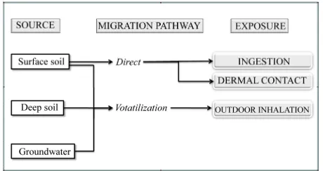
In order to calculate the human health risk caused by the analyzed contaminated site, among all the possible exposure scenarios, the ingestion, dermal contact and outdoor inhalation scenarios are taken into account, as

schematized in the conceptual model in Figure 5. In

performing the human health risk analysis, the receptors

considered as potential targets of the contamination are industrial workers localized on the dismissed area. This choice was dictated by considerations about the actual utilization of the site: since the dismissing of the plant, the ex-industrial area was abandoned, but periodically supervised and subjected to maintenance and numerous monitoring campaigns.

In order to calculate the exposure intakes for the iden- tified receptors, the standard procedures in human

health risk assessment have been utilized [5,16]. The exposure intakes are expressed as mass of substance in contact with the organism, normalized by time unit and body weight (mg/(kg·d)); a summary of the relations used in the procedure can be found in [25].

Human health risk assessment consists in the quanti- fication of Individual Cancer Risk and Hazard Quotient

for the exposed population, i.e. the computation of the

upperbound excess lifetime cancer risk and noncarci- nogenic hazards for each of the pathways and receptors identified in the area of interest. Cancer risk is defined as the probability that a receptor will develop cancer in his lifetime, assuming a unique set of exposure, model, and toxicity properties. In contrast, hazard is quantified as the potential for developing noncarcinogenic health effects as a result of exposure to COCs, averaged over an expo- sure period. It is worth noting that hazard is not a proba- bility but, more exactly, a measure of the magnitude of a receptor’s potential exposure relative to a standard ex- posure level.

The individual cancer risk of a receptor j set by ex-

posure to multiple carcinogenic chemicals i, can be cal-

Figure 4. Benzo(a)pyrene concentration (in µg/m3_{) distribution in air due to the contribution of surface soil, deep soil and}

Figure 5. Conceptual model of the human health risk as-sessment: exposure scenarios.

culated, for low doses exposition hypothesis, through the following equation:

,

_ j i j i

i

Individual CancerRisk 



where:

LADDij is Lifetime Average Daily Dose for a lifetime

exposure of 70 years (mg/kg day) through multiple ex- posure pathways

CSFi is the Cancer Slope Factor for COC i (mg/kg

day)–1_{. Comparing an exposure estimate to a Reference}

Dose (RfD), the potential for noncarcinogenic health effects resulting from exposure to a chemical is evalu- ated. A RfD is defined as a daily intake rate that is esti- mated to cause no appreciable risk of adverse health effe- cts, even to sensitive populations, over a specific expo- sure duration [5]. Generally, the more the Hazard Quo- tient value exceeds 1, the greater is the level of concern. Based on similar COCs toxicological characteristics and additive health effects, the Hazard Quotient (HQ) for receptor j exposed to multiple chemicals i, is calculated as:

,

i j j

i i

ADD HQ

RfD





where ADDijis the Average Daily Dose averaged for the

exposure duration relative to the toxic i for the receptor j

(mg/kg day) through multiple exposure pathways RfDi is

the COC i Reference Dose (mg/kg day) below which

there are no adverse effects. The parameter values adopted for the estimation of the exposure intakes are those typi- cally utilized for the human health risk assessment in the case of workers receptors [26]. The estimation of the exposure time and exposure frequency results from the consideration that the area is dismissed since years and that maintenance works are not requested every day. As a reasonable hypothesis, it has been considered a total number of 1500 hours of exposure for workers receptors.

Table 6 shows the carcinogenicity and toxicity values

of the considered substances utilized for the estimation of Individual Cancer Risk and Hazard Quotient, ex- tracted from U.S. EPA IRIS Database. Summing the con- tribution of all the carcinogenic substances and all the toxic substances, the distribution of total individual can- cer risk and total hazard quotient, respectively, has been

estimated on the considered zone, as represented in Fi-

gure 6(a) and Figure 7(a). As expected, for receptors located and directly exposed on contaminated site, total individual cancer risk has quite high values, especially in the north side of the area. The hazard quotient appro- aches the value of 1 only in a very limited spot of the area.

It’s worth noting that the calculated cancer risk and hazard quotient values don’t take into account any pro- tection of the receptors, thus resulting excessively con- servative and unrealistic. It is evident that workers us- ually use Personal Protective Equipment (PPE) conform- ing to the regulations in force for safety subject during maintenance and monitoring activities in contaminated sites. The use of PPE as gloves and masks can be taken into account in the estimation of risks by considering a reduction factor. As regards the inhalation exposure, if a mask giving protection from dust and gas with mean assigned protection factor is considered, a reduction fac- tor of 1/30 can be supposed (EN 133, EN 529 standards). For dermal contact exposure wearing gloves (EN 374 - 2004 standard) and for ingestion exposure wearing a safety mask, a reduction factor of 1/100 can be conser- vatively hypothesized.

The results consequently obtained adopting the pro-

tection reduction factors are represented in Figure 6(b)

and Figure 7(b), where it is evident an average decrease of risks of about 2 orders of magnitude.

In particular for total individual cancer risk, values above the limit typically considered as threshold accept-

ability, 10–5_{, are almost disappeared, while for hazard}

quotient, values are all reduced under 0.01 estimates. The analysis of the contribution of pathways to both cancer risk and hazard quotient put in evidence that total cancer risk is mainly due to the dermal contribution This assessment can be used as a significant criterion to select the more appropriate PPE in order to reduce risks of exposed workers. In this specific case the inhalation pathway contribution due to volatilization of COCs from soil and groundwater does not constitute the prevailing concern of the contaminated site, but a particular regard has to be posed to dermal contact and therefore to a good choice of safety gloves during maintenance and moni- toring activities on the polluted area.

Table 6. Carcinogenicity and toxicity values for the considered substances.

inhalation ingestion dermal inhalation ingestion dermal CSF

(mg/kg-d)–1 _(mg/kg-d)CSF –1 _(mg/kg-d)CSF –1 _(mg/kg-d) RfD _(mg/kg-d) RfD _(mg/kg-d) RfD

Acenaphtene n.a. n.a. n.a. 0 0.06 0.06

Anthracene n.a. n.a. n.a. 0 0.3 0.3

Benzene 0.0273 0.055 0.055 0.00855 0.004 0.004

Benz(a)anthracene 0.6 0.73 0.73 0.285 0 0

Benzo(a)pyrene 7.32 7.3 7.3 3.135 0 0

Benzo(b)fluoranthene 0.31 0.73 0.73 0.285 0 0

Benzo(g,h,i)perylene n.a. n.a. n.a. 0.03 0.03 0.03

Benzo(k)fluoranthene 0.031 0.073 0.073 0.0285 0 0

Chrysene 0.0031 0.007 0.007 0.03 0.03 0.03

Dibenz(a,h)anthracene 3.1 7.3 7.3 n.a. n.a. n.a.

Ethylbenzene n.a. n.a. n.a. 0.285 0.1 0.1

Fluoranthene n.a. n.a. n.a. 0 0.04 0.04

Indeno(1,2,3-c,d)pyrene 0.31 0.73 0.73 3.14 0.03 0.03

Naphthalene 0.00012 0 0 0.02 0.02 0.02

Pyrene n.a. n.a. n.a. 0.03 0.03 0.03

Toluene n.a. n.a. n.a. 1.43 0.08 0.08

Xylenes n.a. n.a. n.a. 0.2 0.2 0.2

Figure 7. Total Hazard Quotient for workers localized directly on the contaminated dismissed area, without PPE (a) and with PPE (b).

risk benzo(a)pyrene is the main cause, while the hazard quotient is mainly originated by naphthalene, followed by pyrene and chrysene.

4. Conclusions

To quantify the negative effects to receptors exposed to soil and groundwater contamination, human health risk assessment methodology is usually applied, to evaluate individual cancer risk and hazard index. The paper ex- amined in particular the dispersion of contaminant va- pors through volatilization from soil and groundwater in the atmosphere. Volatilization factors have been esti- mated applying Jury’s and Farmer’s models. The sensiti- vity analysis of models, performed with the Sensitivity Ratio, Sensitivity Score and Monte Carlo Simulation, identified the most significant parameters: volumetric water content, thickness of the contamination source and height of capillary zone among the wide range of input parameters for the application of models. Finally a case study regarding a contaminated area located in the indus- trial district of Trento North was investigated. A con- ceptual model of the site was built up, processing the available monitored data; the concentrations of several contaminants in air were evaluated through the estima- tion of volatilization factors. Individual Cancer Risk and Hazard Quotient have been calculated for workers re- ceptors localized on the contaminated site, analyzing the inhalation, ingestion and dermal pathways. In the consi-

dered contaminated site, the volatilization of compounds from contaminated soil and groundwater does not con- stitute the main concern: the dermal contribution results the prevailing pathway for risks and the obtained results can advise the appropriate use of PPE that enable the considerable decrease of the risks for the exposed recep- tors. Adopting conservative reductive factors accounting for the protection of PPE, the resulting individual cancer risks and hazard quotients are clearly below the accept- ability limits.

5. Acknowledgements

We would like to acknowledge the autonomous province of Trento for the support during this study and for pro- viding the monitoring data relative to the contaminated site of Trento North.

REFERENCES

[1] U.S. EPA, “Soil Screening Guidance: Technical Back- ground Document and User’s Guide,” Office of Solid Waste and Emergency Response, Washington D.C., EPA/540/R-95/128, 1996.

[2] ASTM, “American Society for Testing and Materials Standard Guide for Risk-Based Corrective Action Ap-plied at Petroleum Release Sites, E1739-95,” West Con-shohocken, PA, 1995.

[4] J. Grifoll and Y. Cohen, “Chemical Volatilization from the Soil Matrix: Transport through the Air and Water Phases,” Journal of Hazardous Materials, Vol. 37, No. 3, 1994, pp. 445-457. doi:10.1016/0304-3894(93)E0100-G [5] U.S. EPA, “Risk Assessment Guidance for Superfund,

Volume I: Human Health Evaluation Manual. Interim Final,” Office of Emergency and Remedial Response, Washington D.C., OSWER Directive 9285.7-0/a, 1989. [6] U.S. EPA, “Soil Screening Guidance: Technical Back-

ground Document,” 1994.

[7] APAT, “Criteri Metodologici per l’Applicazione Dell’ Analisi Assoluta di Rischio ai Siti Contaminati. rev.2,” Roma, 2008 (in Italian).

[8] ASTM, “American Society for Testing and Materials Standard Provisional Guide for Risk-Based Corrective Action,” Report PS104-98, 1998.

[9] W. A. Jury, W. F. Spencer and W. J. Farmer, “Behaviour Assessment Model for Trace Organics in Soil: I. Model Description,” Journal of Environmental Quality, Vol. 12, No. 4, 1983, pp. 558-564.

doi:10.2134/jeq1983.00472425001200040025x

[10] W. A. Jury, D. Russo, G. Streile and H. E. Abd, “Evalua-tion of Volatiliza“Evalua-tion by Organic Chemicals Residing be-low the Soil Surface,” Water Resources Research, Vol. 26, No. 1, 1990, pp. 13-20.

doi:10.1029/WR026i001p00013

[11] W. J. Farmer, M. S. Yang, J. Letey and W. F. Spencer, “Hexachlorobenzene: Its Vapor Pressure and Vapor Phase Diffusion in Soil,” Proceedings of Soil Science So-ciety of America, Vol. 44, 1980, pp. 676-680.

doi:10.2136/sssaj1980.03615995004400040002x [12] Unichim, “Manuale n.196/01 Suoli e Falde Contaminati,

Analisi di Rischio Sito-Specifica, Criteri e Parametri,” 2002 (in Italian).

[13] RBCA Tool Kit 1.2, “RBCA Tool Kit for Chemical Re-leases,” Groundwater Services Inc., Texas, 1999.

[14] RISC 4.0, “Risk-Integrated Software for Clean-up – User’s manual,” BP-Amoco Oil, Sunbury UK, 2001. [15] GIUDITTA 3.1, “Manuale d’uso/Allegati,” Provincia di

Milano-URS Dames and Moore, 2006 (in Italian). [16] U.S. EPA, “Risk Assessment Guidance for Superfund:

Volume III—Part A, Process for Conducting Probabilistic Risk Assessment,” OSWER 9285, EPA 540-R-02-002, 2001, pp. 7-45.

[17] Decisioneering, Inc., “Crystal Ball ® User Manual,” 2005 [18] R. F. Carsel and R. S. Parrish, “Developing Joint

Prob-ability Distributions of Soil Water Retention Characteris-tics,” Water Resources Research, Vol. 24, No. 5, 1988, pp. 755-769. doi:10.1029/WR024i005p00755

[19] J. A. Connor, C. J. Newell and M. W. Malander, “Pa-rameter Estimation Guidelines for Risk-Based Corrective Action (RBCA) Modeling,” NGWA Petroleum Hydro-carbons Conference, Houston, November 1996.

[20] M. Th. Van Genuchten and P. J. Wierenga, “Mass Trans-fer Studies in Sorbing Porous Media: I. Analytical Solu-tion,” Soil Science Society of America Journal, Vol. 40, No. 4, 1976, pp. 473-480.

doi:10.2136/sssaj1976.03615995004000040011x [21] M. Th. Van Genuchten, “A Closed-Form Equation for

Predicting the Hydraulic Conductivity of Unsaturated Soils,” Soil Science Society of America Journal, Vol. 44, No. 5, 1980, pp. 892-898.

doi:10.2136/sssaj1980.03615995004400050002x [22] E. L. Lehmann, “Nonparametrics: Statistical Methods

Based on Ranks,” New York, Springer, 2006.

[23] G. Andreottola and C. Simonini, “Test di Ozonizzazione in situ di Terreni Contaminati da IPA. Risultati Preliminary,” Proceedings of Conference in “Nuovi Indirizzi Nella Bonifica dei siti Contaminati - La Prassi, la Normativa, le Nuove Tecnologie,” Provincia di Milano, 2004 (in Italian).

[24] C. W. Fetter, “Applied Hydrogeology,” 3rd Edition, Prentice Hall, Engelwood Cliffs, 1994.

[25] P. Morra, S. Bagli and G. Spadoni, “The Analysis of Human Health Risk with a Detailed Procedure Operating in a Gis Environment,” Environment International, Vol. 32, No. 4, 2006, pp. 444-454.

doi:10.1016/j.envint.2005.10.003

Notation

δair ambient air mixing zone height

ρs soil bulk density

θa volumetric air content

θa,cap volumetric air content in the capillary zone

θe effective terrain porosity in unsaturated zone

θw volumetric water content

θw,cap volumetric water content in the capillary zone

τ average duration time of vapor flux A contamination source area

ADD Average Daily Dose averaged for the exposure duration cpoe pollutant concentration in point of exposure

cs pollutant concentration at the contamination source

COC Chemical of Concern CSF Cancer Slope Factor

d thickness of contamination source in the surface soil ds thickness of contamination source in the deep soil DA diffusivity

Dadiffusion coefficient of the substance in air

Dcapeff effective diffusion coefficient through capillary zone

Dw diffusion coefficient of the substance in water

Dseff effective diffusion coefficient in soil based on vapor-phase

concentration

Dwseff effective diffusion coefficient between the groundwater

and soil surface

foc organic carbon fraction H Henry’s law constant hcap height of capillary zone

hv height of unsaturated zone

kd partition soil-water coefficient

kOC carbon-water partition coefficient

kssoil-water sorption coefficient

L extension of contamination source in across-wind direction LGW depth to groundwater

Ls depth to subsurface soil contamination source

LADD Lifetime Average Daily Dose for a lifetime exposure of 70 years

RfD Reference Dose

Uair wind speed above the ground surface in the ambient

mix-ing zone

VFss volatilization factor of outdoor vapors from surface soil

VFds volatilization factor of outdoor vapors from deep soil

VFgw volatilization factor of outdoor vapors from groundwater