Modelling of High Frequency Roughness Scattering from Various Rough Surfaces through the Small Slope Approximation of First Order

Modelling of High-Frequency Roughness Scattering from

Various Rough Surfaces through the Small Slope

Approximation of First Order

Virginie Jaud1_{, Cedric Gervaise}2_{, Yann Stephan}3_{, Ali Khenchaf}1 1_{Passive Acoustics, Superior National School of Advanced Techniques of Brittany, Brest, France}

2_{GIPSA-LAB, SIGMAPHY, French National Centre for Scientific Research, Grenoble, France} 3_{The Naval Hydrographic and Oceanographic Service, Brest, France}

Email: [email protected]

Received November 22,2011; revised December 24, 2011; accepted January 10, 2012

ABSTRACT

The first-order small slope approximation is applied to model the scattering strength from a rough surface in underwater acoustics to account for seafloor for high frequencies from 10 kHz to hundreds of kilohertz. Emphasis is placed on simulating the response from two-dimensional anisotropic rough surfaces. Several rough surfaces are described based on structure functions such as the particular sandy ripples shape. The scattering strength is predicted by the small slope approximation and is first compared to a well known bistatic method, interpolating the Kirchhoff approximation and the small perturbations model, assuming that the rough interface is isotropic. Results obtained from the two different mod-els are similar and show a higher level in the specular direction than in the other directions. For an isotropic surface, changing the propagation plane gives similar results. Then, SSA, which lets us adapt the structure function of the roughness straight away, is tested trough several anisotropic surfaces. In a longitudinal direction of ripples, the scatter-ing strength is mostly in the specular direction, whereas in the transversal direction of ripples, the scatterscatter-ing strength prediction shows high values for different angular directions. Thus the scattering strength is spread in a very different way strictly related to the particular features of the ripples. Combine our results, indicates the importance of taking into account the anisotropy of a surface in a scattering prediction process, taking into account the positions of the emitter and of the receiver which are naturally significant when predicting scattering strength.

Keywords: Anisotropy; Roughness; Scattering; Small Slope Approximation

1. Introduction

Acoustics scattering from the ocean bottom is a subject of interest for many remote sensing acoustic sensing ma- rine activities, such as classification of seabed, or map- ping of ecosystem habitat [1,2]. To these purposes, high frequency tools, as single beam or multibeam echosound- ers or side scan sonars, are used to assess the bottom rou- ghness and improve the knowledge of the environment [3,4]. However if such systems can generally provide a detailed image of the bottom, the relationship between the acoustic measurements and the physical parameters of the bottom is strongly dependent on the type of envi- ronment, and in particular the type of bottom roughness. To gain more insights into scattering phenomena, it is needed to develop and use pertinent scattering models considering the roughness of seabeds. The investigation of the interest and efficiency of one of these models, the so-called Small Slope Approximation (SSA) is addressed in this paper. This choice has been made based on the

possibility of taking into account different types of rough surface as well as due to the direct link between rough- ness and scattering which of importance in a perspective of roughness inversion, thus for predicting roughness trough scattering data.

for monostatic cases and isotropic rough seafloors. Jack- son and coworkers [10-12] have modified the monostatic method to obtain a bistatic model which only works for isotropic surfaces. This model can be seen as the inter- polation between to other models, the Kirchhoff ap- proximation (KA) and the small perturbations method (SPM). KA predicts scattering in the specular direction whereas SPM is used for predicting in the other direc- tions. This model was used by Choi et al. [13,14] for com- paring theory with real data obtained from their meas- urements above ripple field. Nevertheless their compare- sons showed that the orientation of the measurement pla- ne compared to the direction of the ripples has a great ef- fect on the scattering. Thus they conclude on the need of considering the anisotropic state of a surface into the scat- tering process.

To take into account the anisotropy of the seabed, which is the basic motivation of this paper, the small slope approximation, originally developed by Vorono- vich [15], is interesting since it allows to consider vari-ous anisotropic rough interfaces via the two-dimensional structure function. This method has been elaborated as a unifying method able to reconcile small perturbations method and Kirchhoff approximation [16]. Theoretical expressions have been developed at different orders by Thorsos and Broschat in [17,18] without taking into ac- count quasi-periodic seafloors and further studied by Gragg et al. and Jackson et al. [19,20] in the case of iso- tropic interfaces.

The main concern is to better understand how a sandy sediment with directional features can impact the acous- tic propagation and scattering by using the SSA and by modifying the roughness structure of the seafloor. For instance, ripples, which are close to a periodic surface, are a complicated type of rough interface. They are not always perfectly periodic, They may be dependent on particular parameters like currents and/or waves, their shape changes with time, and so on. Experiments have already been done to measure such surfaces under certain conditions [21], whereas theoretical descriptions of rip- ples are not global and are different from one type of ripples to another. For modelling the seafloor, a random process is assumed and depends on a height covariance which takes into acount particular features of the wanted rough surface. Characteristics of the rough surface are, for instance, related to rms-height, to the correlation len- gths in different direction, to the wavelength of the sine shape function, and so on, depending on the height co- variance of interest.

This paper is organized as follows. Section 2 describes the configuration of the scattering problem, shows in details how the roughness of a relief is taken into account in the scattering process and the main expressions of the small slope approximation are described. The structure

function is directly related to the scattering method. In Section 3, different rough surfaces are evaluated. The small slope approximation is used with different types of reliefs, from the simplest case to a more complicated ca- se: first an isotropic surface is tested, based on sediment parameters, often used for dealing with isotropic sedi- ment, that is why the method is compared to another one, chosen as a reference. The results validate the use of the small slope approximation in this isotropic test case. Then results are obtained from different anisotropic cases, one from a surface based on a Gaussian distribution, second from a rough surface interface with a quasi-periodic shape we developed. We finally discuss the effects of the relief on the predictions of the roughness scattering strength.

2. Modelling of Scattering Strength from a

Rough Surface

2.1. Context and Geometry

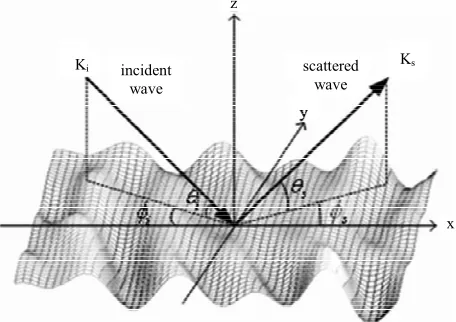
The geometry of the scattering model is depicted in Fig-ure 1 in terms of incident and scattered waves.

ki and ks are respectively the incident and scattered

wave vectors.



, kzi



 

i i

k K (1)



, kzs



 

s s

k K (2)

where Ki and Ks are the transverse components of the

incident and scattered waves in the (x, y)-directions, so





i xi yi

K  k , k and Ks



k , kxs y





s . These wave

com-ponents depend on the acoustic wavenumber, k, on the grazing incident angle _i 0 ,90 



and on the grazing scattered angle s



0 ,180 



. The azimuth angles are

incident wave

scattered wave z

Ki Ks

[image:2.595.308.536.505.666.2]

x

Figure 1. Configuration of the scattering problem with the incident wave vector i, the scattered wave vector ks, the

grazing incident angle θi, the azimuth incident angle i

k

, the grazing scattered angle θs and the azimuth scattered angle

s

where C

 

r and C

 

0 are respectively the height co- also taken into account and change with positive

anti-clockwise angles



 i, s







0 ,180 



in our simulations.

The vertical component in the z-direction, kzi and kzs,

variance at the position r and at zero lag. The two-di- mensional covariance is defined as follows.

respect 2



2 2



z x

k  k  k k_{y . These terms are used to} C

 

r h



r r

  

h r (5) with the mean and r the lag. One should notice that for a zero lag the autocorrelation is equal to 1 for

 

C r divided by its variance. solve the scattering problem from a rough surface which

statistical descriptions follow. Figure 2 shows examples of various angular configurations of interest for the dif-

ferent simulations presented in Section 3. One of the most typical isotropic structure functions is based on the grain sediment [9-12]. It is parameterized by a power-law spectrum and is defined by the following expression

2.2. Modelling of the Isotropic and Anisotropic Surfaces via the Structure Function

 

 

2π Γ

_

2



2

_{ }



2 2

_

2

1 Γ 1

i i

w

D D r r

 



  

 

 

 

r (6)

The water and the seafloor are separated by a rough in-terface. In our context, this surface is considered plane on the average and is defined as

where r is the distance, w2 the spectral strength,



2 2 2



   with 2 the spectral exponent Γ is the

gamma function. Nevertheless, to be able to change the roughness by modifying the correlation lengths, Lx and Ly

respectively in the x- and y-directions, and the rms-

height of the surface directly, two main structures func-tions are of interest in this study. One of the structure function, Dg is based on a Gaussian distribution. This type

of distribution is well known when simulating scattering strength from a rough surface [6,8].

 

z h r (3)

where r

 

x y, is the position on the



x y,



-plane, h

is the deviation of the interface relative to its means plane , z is usually considered as a random process. To take into account the relief, its isotropic or anisotropic feature, when simulating scattering strength by a rough surface, the structure function is defined by Equation (4).

0

z

 

 



D r C 0 C r



(4)

(y,z)-plane

φi= 90°

φs= 90°

(x,z)-plane

φi= 0°

φs= 0°

z

x z

2 1.5 1 0.5 0 –0.5 –1 –1.5 –2 –2 –1.5 –1 –0.5 1 0.5

0 1.5 2 –0.02 –0.01 0 0.01 0.02

0 0.05

1

0.5

0

–0.5

–1 –1

–0.5 0

0.5 1 2 1.5 1 0.5 0 –0.5 –1 –1.5 –2 –2 –1.5 –1 –0.5 1 0.5

0 1.5 2 –0.010 0.01

2 1.5 1 0.5 0 –0.5 –1 –1.5 –2 –2 –1.5 –1 –0.5 1 0.5

0 1.5 2 –0.02 –0.01 0 0.01

0.02

[image:3.595.124.475.387.666.2]

–0.02

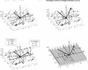
Figure 2. Angular configurations for different cases of interest: (top left) configuration for an isotropic surface as a function of the scattered angle s; (top right) configuration for an isotropic surface as a function of the scattered azimuth angle s;

(bottom left) configuration for an isotropic surface as a function of the scattered angle s into two different planes, the (x,

z)-plane for  i= s=0and the (y, z)-plane for  i= s=90; (bottom right) configuration for an anisotropic surface as a

 

2 2 2 2 2

2 1 e x y

x y

L L

g rms

D h

 

 



 _ 

 

 

r _ (7)

The structure function Dg is used either to model an

isotropic surface or an anisotropic surface, depending on the values applied to the correlation lengths, Lx and Ly,

respectively in the x and y directions. To deal with a part of periodicity and directionality of an interface, such as sandy ripples, we suggested another structure function,

Dp which is based on a sine function.

 

 

 





2 2

2 2π

2 1 cos cos sin e x y

p

x y

L L

rms p p

p

D

h  x  y



 

 _

 

   _ 

 _

 r

 

 

 _

(8) The structure function Dp is used to model a rough

surface with periodic features, thus the surface is anisot- ropic and respect few statistical properties but mandatory such as the second-order stationary of the surface and that the surface is ergodic. In case of ripples, we assume that they do not change due to a particular event. Sur- faces based on this structure function are in the following of this paper called ripples. The termspandpare

re-spectively the angle for the direction of the periodic sine shape and the wavelength of the sine function. The cor-relation lengths Lx and Ly allow to get a rough surface

with periodic features more or less disordered.

Combining the three different structure functions al- low us to simulate particular rough seafloors for predict- ing scattering strength. is appropriate for a ran- dom rough surface made of a sediment which roughness properties have been estimated [10,12]. is ap- propriate either for testing isotropic or anisotropic rough surfaces but without any feature about directionality or periodicity. Thus Dp which takes into account a quasi-

periodic rough surface, is of interest since the effect on an acoustic wave is expected to be different from other types of anisotropic surfaces, and would give relevant information concerning the approach used to analyze the effect of sandy ripples.

 

i

D r

 

g

D r

To get one realization of a surface based on one of the previous structure functions, thus on one of the height covariances, first a Gaussian white surface is produced. Then its Fourier transform is weighted by the square root of the spectrum based on a chosen height covariance. Finally, the inverse Fourier transform gives one realiza- tion of the rough surface. The process to get a relief is summarized by Equation (9)

 

_{r F}1 _F

 

_{F B}

 

h _   _C _ 

 

 

 r  

where F is the Fourier transform, F–1 _{the inverse Fourier}

3 shows one realization of an isotropic surface ba

sotropic sur-fa

ation of an anisotropic sur-fa

(9)

[image:4.595.120.223.87.130.2] [image:4.595.335.510.349.486.2] [image:4.595.334.510.545.687.2]

transform and B a Gaussian white noise. As an illustra- tion, we present in the following three examples of rough surfaces.

Figure

sed on a Gaussian distribution which features are similar for all (x, y)-directions. Thus for such a surface, scattering model can be simplified from a two dimen-sional problem to one dimendimen-sional case.

Figure 4 shows one realization of an ani

ce based on a Gaussian distribution, but with different features depending on the direction. In the y-direction, the correlation length is longer, thus the surface has got a smoother shape compared to the x-direction where the correlation length is smaller.

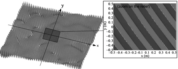
Figure 5 shows one realiz

ce based on the structure function Dp

 

r . Other hei-

ght fluctuations are observed. They ar to the expo-nential part of the structure function and they are related to the choice of very long correlation lengths versus

e due

p



in this case. The direction and the periodicity of the relief depend on p and p respectively.

Figure 3. One realization of an isotropic surface, 5 m 5 m, × based on a Gaussian distribution (i.e. height covariance re- lated to the structure function Dg(r)), with Lx = Ly = 20 cm,

hrms = 5 cm.

Figure 4. One realization of an anisotropic surface, 5 × 5

rms

m m, based on a Gaussian distribution (i.e. height covariance related to the structure function Dg (r)), with Lx = 20 cm, Ly

[image:5.595.114.484.85.229.2]

Figure 5. One realization of an anisotropic surface, 5 m × 5 m, based on a sine function (i.e. height covarianc elated to the structure function D(r)), with L = L = 300 cm, h = 5 cm, λ = 20 cm, φ = 30˚.

n

odelling of Scattering Strength with SSA-1

e r

p x y rms p p

In the following simulations with such a type of relief, lo ger correlation lengths i.e. Lx Ly 100 m will be used to get a large surface mostly dependent on the sine shape.

2.3. M

The scattering problem is analyzed trough the scattering strength, SS, which is defined in decibel (dB) as:







_

_











10

10

,

, , , 10 log Is s s

SS         

,

10 log , , ,

i i s s

i i i

i i s s

I m

     

 

 



(10)

where I_i is the incident intensity, I_s is the scattered intensity and m is the dimensionless scattering coefficient. The latter parameter represents how the acoustic wave is scattered from the rough surface (ref. at 1 m-distance over a 1 m2 _{surface). In this study, m is evaluated by}

us-ing the first-order small slope approximation [12, 15,17,19] and is written as :













   2    2 _{ }

2 4

2 2

1 1

·

2 2

, , ,

i i s s

m   

, , , 4π

e e d d

zs zi zs zi

spm i i s s

zs zi

k k D k k D _i

k A

k k

e x y

   

   

  _{     }



   

 





 

   

 

 



r K r

(11) whereK





kxskxi



, k



yskyi





is the wavevector difference, r

 

x y, is the position on the

 

x y, -plane

and D

 

r is the structure function defined in the pre-viou (see Equation (4)). In this study, scattering from sediment volume and multiple scattering are not considered, whereas losses of energy due to trans- mission into the sediment (from homogeneous or strati-

s section

fied seafloor) are considered through Aspm



   i, , ,i s s



.

Assuming that the sediment is fluid, this parameter de- pends on the plane wave reflection coefficients and on the incident and scattered waves as Equation (12) [12,22]. where  is the density ratio between sediment and wa-ter,  is the wavenumber ratio between sediment and water, R is the plane-wave reflection coefficient depend-ing either on the grazdepend-ing incident angle i or on the

grazing scattered angle s. One should note that the

first-order small slope approximation coefficient could be shared into two major parts. Before the integral in Equation (11), sediment characteristics are defined, thus losses due to sediment are taken into account. Then the integral is related to the roughness of the seafloor which is the cause of the surface scattering phenomenon.

Concerning the choice of the roughness into the scat- tering model, our interest is to change easily the type of roughness when predicting scattering. The small slope approximation allows us to modify directly the height statistics, either by using true measurements of a rough surface or by using theoretical model to describe the ap-proximation of first order is compared to a well-known bistatic method based on an isotropic surface, thus the effect of the isotropic roughness are shown. Then, SSA-1 is analyzed based on an anisotropic rough surface ob- tained by a Gaussian distribution. Finally, the model is used with another anisotropic roughness we suggested in





 

 

   

2

2 2

2 2

2

, , ,

· 1 ( ) 1

1 1

1 1 1 1 sin sin

4 1

spm i i s s

s i

s i s i

s i

A

R R

R R

R R

k    

 



    

   

 _{( )} 

( ) 1 ( )

     

 

   

         _  _ _K Ks i _{ }  _{  } __

roughness. This modelling approach differs from many computations where anisotropy is directly implemented in the scattered field. The advantage of providing the roughness straightaway is also related to the unique limi- tation of SSA of first order: the elevation slopes have to e small enough. This is an asset compared to other

the scattering strength obtained with

r structure function described by Equa- atic SA

and analyzed

Then b

tering models where limitations are more numerous. To avoid shadow at very small grazing angles, higher orders of the SSA method could be considered [17,18]. Never- theless the model of first order is relevant because the scattering coefficient is directly related to the roughness statistics and makes a roughness inversion process possi- ble. In order to keep this ability and to take into account the limitation, the validity area compared to the type of roughness should always be kept in mind when analyzing the scattering data.

3. Simulations: A Parametric Study

This section is organized as follows: first the small slope this paper. The anisotropy of a rough surface is first ex- amined, then the complexity of the anisotropic roughness is enhanced through

SSA-1.

3.1. Study 1: Analysis of SSA-1 Compared to Jackson et al. Model (Case of Di(r))

The small slope approximation is used to predict rough- ness scattering from an isotropic surface based on the particula Di

 

r

tion (6) and always used in prediction by the bist model developed by Jackson et al. [11,12]. Both S

Jackson et al. models are first compared to

the efficiency of SSA-1 assuming a basic environment made of sediment (fine sand or coarse sand) and based on an isotropic rough surface. scattering predictions are performed into different propagation planes, through a change of the scattered azimuth angle, to examine the properties of isotropy on scattering strength.

Two types of sediment, fine sand and coarse sand, are used as examples. The properties of these sediments are given in the following Table 1.

Figure 6 shows the prediction of the scattering stren- gth, SS, as a function of the scattered angle _s in one plane such as  i s0, for two kinds of sedi

s) and ments, fin

ith symbol com- pa

e sand (lines with circles) and coarse sand (line with squares). The predictions of the roughness scattering are made with SSA (dashed line w

red to the bistatic model developed by Jackson et al. (full line with symbols) [11]. First of all, for two types of sediment and fo ifferent models, the scattering strength is higher in the specular direction for s i

r the two d

 

[image:6.595.305.539.98.389.2]

and decreases to a minimum value at grazing scattered angles. Then, apart from the specular direction and due to the particularity of each sediment (roughness dimensions

Table 1. Sediment parameters.

Parameters Fine sand Coarse _sand

density ratio ρ 1.451 2.231

compressional sound speed cp[m/s] 1660 1876

loss parameter δp 0.01602 0.01638

roughness spectral exponent γ2 3.25 3.25

roughness spectral strength w2 m42 8.6 × 10–5 2.2 × 10–4

Figure 6. Predictions and comparisons (SSA-1 versus the bistatic Jackon’s model) of scattering strength, SS, as a function of the scattered angle θs for coarse sand (lines with

squares) and for fine sand (lines with circles) for f = 30 kHz,

θi = 30˚, φi = φs = 0˚.

and losses), the scattering strength is mainly higher for a coarse sand than for a fine sand. For both types of sedi- ment, predictions are very close between SSA and the other bistatic model for most of the scattered angles. The small differences, about less than 2 dB, appear at par-ticular scattered angles around  s 20 and around

s 60

   for these test cases. One should notice that the bistatic model developed by Jackson et al. is based on the interpolation of both the Kirchhoff approximation and the small perturbations method (KA being used in the specular direction and SPM in the other directions). The change from KA to SPM appear, in these simulated pre-dicttions at scattered angles approximately around  s 20

and around  _s 60, which match the angles where differ-ences were found. The small slope approximation being a unified method, small variations may be observed at the particular angles of interpolation of the other method.

Figure 7 shows the predictions of scat ering strength as a function of azimuth angle s

t

Figure 7. Predictions and comparisons (SSA-1 versus the bistatic Jackon’s model) of scattering strength, SS, as a function of the scattered azimuth angle φs for coarse sand

(lines with squares) and for fine sand (lines with circles) for f = 30 kHz, θi = θs = 30˚, φi = 0˚.

sand and fine sand, and for the two different models, the scattering strength is higher at very low azimuth angles, with a maximum value for  s 0

en th nd than fo

from a

wavel r than th

ic mod

which match with the specular direction. Th e scattering strength is mainly higher for a coarse sa r a fine sand, par- ticularly in a direction away the specular direction and this feature has to be rel ted to the roughness char

ength, the sediment ade of fine sand is smoothe e coarse sand, thus - acteristics of each sediment (coarse sand rougher than fine sand) as well as to the losses parameters (fine sand at- tenuates acoustic waves more than coarse sand). For one given frequency, i.e. one given

m

the energy is spread in more directions for the coarse sand case. Finally, both predictions from SSA and pre- dictions from the other bistat el are very similar, especially at angles equal to the specular angle (around

s 0

  ) and at scattered azimuth angles higher than 60˚. Small differences, less than 2 dB, appear at azimuth scat- tered angles around  _s 30. These angle area match the ones corresponding to the interpolation between KA and SPM.

Similarities of the simulations and very small differ- ences of the same kind have been observed for other si-mulated cases where the type of sediment, or the fre- quency, and so on, were modified. Contrary to the bista- tic model developed by Jackson et al., the small slope approximation is a unified method of the KA and SPM characteristics, that is why comparisons between SSA other bistatic model were first of interest. Then one advantage of the small slope approximation, through the expression given tion (11), is that different structure functions can be implemented directly with this model. Com

and the

by Equa

bine these primary results, based on an

iso-tropic surface, allows to implement more complicated seafloors in the scattering process through the other structure functions Dg

 

r and Dp

 

r .

3.2. Study 2: Analysis of SSA-1 with an Anisotropic Surface

3.2.1. Case of a 2-D Gaussian Structure FunctionDg(r)

A Gaussian distribution through the structure function Dg

is first used to model roughness (see the corresponding relief in Figure 4). The correlation length in the x-direc- tion varied from the one in the y-direction such as

kLx 12 and kLy 20. The variations of the height

are taken into account in kh = 1.5 with k the wavenumber. For a fixed value of kh, Lx and

ing as a function of the scattered angle

k kLy respect the limita-

[image:7.595.58.287.84.264.2] [image:7.595.307.538.504.675.2]

pes [18]. s scatter- tion of SSA, that is assuming small surface slo

Figure 8 shows the prediction of the roughnes

s

 ,  i 70, i s

into two different planes, in the (x, z)-plane with   0,

th

and in the (y, z)-plane wi  _i _s 90 (see Figure 2

for the angular configurations of the planes). For predic-tions into the two different planes, the maximum value is obtained in the specular direction for  _s _i 70. Then the scattering strength decreases to a minimum values

at graz s. In the (y, z)-plane of Figure 8, the scattering strength covers a narrow band around 70˚, such as an scattered angle area about 30˚ at –10 dB. In the (x, z)-plane, the energy is spread in more directions, such as the scattered angle area is equal to 80˚ at –10 dB. This phenomenon follows the expected b ha in the direction where the surface is smoother, the scattered energy is distributed around the specular direction whereas for rougher surfaces, the energy is spread in more direc- tions.

obtained ing angle

e viour:

Figure 8. Prediction of scattering strength, SS, as a function of the scattered angle θs, for θi = 70˚; (line with circles) φi =

φs = 0˚ thus for a plane where the correlation length is

smaller kLx = 12; (line with squares) φi = φs = 90˚ thus for a

[image:8.595.58.286.489.674.2]

Figure 9 shows the scattering predictions, SS, as a function of the azimuth angle s , and depend on

i s 70

    and  i 0

ation lengt

. Two sim lations are compa- red. One is based on the anisotropic surface used previous-

rel hs are 2 and 0

u

x

L

ly which cor k 1 kLy2 .

ropic surface, both the

12 The second

such as co

x-direction a

simu sed

rrel hs ilar in

nd t -direction, with lation is ba

ation lengt he y

on an are sim

isot

kL_xkL_y . For d in the

a ximum

the isotropic c specular direct

se, the ma ion for s

value is obtaine 0

   and decreases with higher values of s. The scattering e

180

str ngth shows a minimum values for  s

obtained in



case, the m , thus in the

axim

backward value

direction. For scattering

s 0

the anisotropic strength is

um

the specular direction of the

for   , then it decreases to a minimum around  _s 100 and finally increases in the backward direction for  s 180.

Nevertheless, the value in the backward direction (–22 dB at  s 180) is much lower than the value in the specu-

lar direction (about –5 dB fort  _s 0). The scattering strength is spread differently between simulations with an isotropic surface and with an anisotropic surface. The scattering strength is slightly higher in the specular direc-tion, between  s 0 and  s 25, of the anisotropic

case, as well as for azimuth angles between  _s 150

and  s 180. On the contrary, between  s 25 and s 150

  , scattering strength from the anisotropic case is lower than from the isotropic case, with 10 dB differ-ence at  _s 90.

In the isotropic case, the scattering problem could be simplified to one direction which is not suitable in the anisotropic case since the entire surface induces an effect on the roughness scattering phenomenon.

Figure 9. Prediction of the scattering strength, SS, as a function of the scattered azimuth angle φs, with θ = θ = 70˚,

= 0˚; (line with circles) different correlation lengths i s Lx≠ y, (kLx = 12 and kLy = 20); (line with squares) Lx = Ly, (kLx

= kLy = 12).

3.2.2. Case of a 2-D Quasi-Periodic Structure Function Dg(r)

The third type of structure function is now used for si-mulating the small slope approximation (see the corre-sponding relief in Figure 5) in the case of a quasi-perio dic relief such as a sandy bottom made of ripples. Scat- tering predictions are based on the structure function D

defined by Equation (8), with a wavelength of

φi

L

p

p 20 cm

  , a rms height of 5 cm, a zero deviation angle of _p0 m. The inci-and large correlation lengths

dent wave is defined by

100

x y

L L 

60

i  

pre of the

tw ), with

 and a frequency dictions of th scattered angle o planes, in th

i s 0

of 50 e scattering

s

θ . Scatter- e (x, z)-plane kHz. Figure 10 shows

strength as a function ing strength is given into

(dashed line in Figure 10    Figu

, and in the

re 10) with (y, z)-plane (line with squares in

i s 90

   . One should note that, in this test case, the (x, z)-plane in the transversal direction of the ripples (the acoustic waves propagate perpendicularly to the ripples directions) whereas the (y, z)-plane is in the longitudinal direction of the ripples (the acoustic waves pr

parallel to the ripples directions). Configurations o gation planes are

opagate f these propa depicted in Figure 2.

The scattering strength shown in Figure 10 and de-pending on the (y, z)-plane, is spread in a narrow band around 60˚ (about 5˚ at –10 dB), which is the specular direction. In this direction, the surface is much smoother and mainly depend on the correlation length Ly100 m.

Such a scattering behaviour, most of the acoustic spread in the specular direction, is expected for a smooth surface. Then in the (x, z)-pla , the scattering strength varies strongly as a function of the scattered angle _s

energy

ne

[image:8.595.307.538.496.674.2]

 , with eleven maximum values around 10 dB down to –40 dB in this test case. The variation from one maximum

Figure 10. Prediction of the scattering strength, SS, as a function of the scattered angle θs, θi = 60˚; (dashed line) φ =

φs = 0˚ thus propagation plane in the transversal direction

to the ripples; (line with squares) φi = φs = 90˚ thus

propa-gation plane in the longitudinal direction to the ripples.

value to one minimum one is very fast, about 5˚ of dif-ference to go from one extreme value to the other. Fur-thermore, the angular lag between two maximum scat-tering strengths is approximately 10˚, particularly for scattered angles between  s 50 and  s 150

ned for . It in-creases a bit for scattering strengths obtai  _s 50

and  s 150. These

[image:9.595.57.287.499.685.2]

shape of the roughness and thus through its structure function since the acoustics wavelength (3 cm for 50 Hz) is of order of the ripples dimensions (rms height of 5 cm and wavelength of 20 cm).

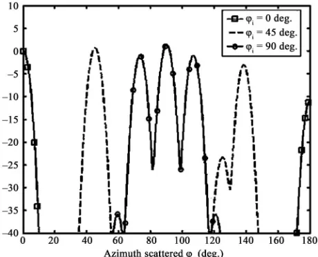
Figure 11 shows scattering strength, SS, as a function of the azimuth scattered angle

variations can be related to the

s

 for three different azimuth incident angles i0,  i 45 and  i 90

θs =θi =

r the angu-. The incident and scattere d by

60˚ with a 50 kHz-freque fo d an

ncy (see

gles are define

Figure 2

lar configuration). The rough surface is similar to the quasi-periodic sandy ripple relief used in the previous simulation, based on the structure function Dp defined by

Equation (8), with a wavelength of p 20 cm, a rms

height of 5 cm, a zero deviation angle of p0 and

large correlation lengths L_xL_y100 m.

For i 0, most of the energy is spread in the

for-ward direction (around the specular direction for s 0)

and in the backscattering direction (i 180 For an

incident wave at i 45, maxima are around

and

).

s 45   

s 135

  , which are respectively the forward and the backward directions. For i90 a maximum stren-

gth appears at _s90 which is the forward direction, and also at 70˚ and 110˚. They correspond to positions of the scattered wave between the transversal and the lon- gitudinal directions of the quasi-periodic relief. In this simulated case, the scattering strength is still higher if

Figure 11. Prediction of the scattering strength, SS, as a function of the scattered azimuth angle φs, θs = θi = 60˚; (line

with squares) φi = 0˚; (dashed line) φi = 45˚; (line with circles)

φi = 90˚.

incident and scattered waves are in a same plane, the amount of energy spread in the backward direction is also important and scattering strength appear also in di- rections which are out from the forward and backward ones. Compared to the previous anisotropic case, the dis- tribution of energy is different and is closely related to the structure function which has been modified from a Gaussian case to a quasi-periodic case. Thus directional- ity and periodicity of a seabed seem to be relevant on the scattering strength distribution.

4. Discussion

The first order small slope approximation is used to pre-dict sound scattering by an anisotropic rough surface. With this model, we address the effects of seabed rough- ness with particular attention being given to simulation

y to change the roughness structure, either by

smoother direction of the surface, the scattering strength obtained considering one would be spread around the specular

he scattering strength is predicted differently fr

of the two-dimensional height structure function. The model is restricted by the usual small slopes assumptions, e.g., no sharp edges. The interest of this model is the possibilit

using measured heights or theoretical heights. The re- placement of such a surface by the one used in this study with a directional feature enhances the complexity of the numerical integral of SSA but expands the field of appli- cations.

Predictions of the scattering strength from an anisot- ropic surface based on Gaussian distribution have shown that the choice of the positions of a source and a receiver compared to the rough isotropic surface is important and give different information. In a

propagation plane

direction. On the contrary, for a propagation plane placed in a rougher direction, the scattering strength is spread in more directions. For an anisotropic surface, the entire two-dimensionnal statistics of the surface should be kept instead of simplifying the model, to avoid inaccurate es- timation of the scattering strength. Furthermore, assume- ing an unknown surface, the differences obtained in the different propagation planes may be of interest for analy- zing the seafloor from the scattering strength data. Then, combine results obtained from the anisotropic surface based on a quasi-periodic structure function, indicate as well the importance of taking into account the anisotropy in a model used for estimating the scattering energy dis-tribution. T

the same level and thus for different scattered angles. In this case, for a propagation plane in the transversal direc- tion of the ripples, the specular direction is not the direc- tion of interest. On the contrary, this direction is of im- portance for the simulations made in the propagation plane in the longitudinal direction of the quasi-periodic shape. Again, the results show the effect of choosing the position of the emitter and receiver compared to the rou- ghness of the surface. Nevertheless, these very high-chang- ing values, predicted by SSA-1 should be minimized in practice, since sonars or transducers depend on their own directivity, thus give an average value of the scattering strength.

Simulations and literature have shown the requirement of combining directionality of the anisotropy in the scat- tering model to correctly predict scattering strength in all directions. To better analyze these conclusions, tank ex- periments are required in order to model the appropriate structure function and validate the scattering process de- scribed in this paper, since data obtained from a control- led environment are always of interest to better under- stand a physical problem. It would be word worth also predicting roughness instead of roughness scattering via

the structure function by extraction of this component.

5. Acknowledgements

This work was partly funded by the French Defence Pro-curation Agency (DGA) under research program ERATO (contract 09CR0001).

REFERENCES

[1] J. T. Anderson, D. Van Holliday, R. Kloser, D. G. Reid and Y. Simard, “Acoustic Seabed Classification: Current Practice and Future Directions,” ICES Journal of Marine

Science, Vol. 65, No. 6, 2008, pp. 1004-1011.

doi:10.1093/icesjms/fsn061

[2] A. J. Kenny, I. Cato, M. Desprez, G. Fader, R. T. E. Schüt-tenhelm and J. Side, “An Overview of Seabed-Mapping Technologies in the Context of Marine Habitat Classifica-tion,” ICES Journal of Marine Science, Vol. 60, No. 2, 2003, pp. 411-418.doi:10.1016/S1054-3139(03)00006-7 [3] K. Siemes, M. Snellen, D. G. Simons, J.-P. Hermand, M.

Meyer and J.-C. Le Gac, “High Frequency Multibeam Echosounder Classification for Rapid Assessment,” Acous-tics’08, Paris, 29 June-4 July 2008, pp. 4259-4264. [4] L. Hellequin, J.-M. Bouch

of High-Frequency Multi

er and X. Lurton, “Processing beam Echo Sounder Data for Seafloor Characterization,” IEEE Journal of Oceanic En- gineering, Vol. 28, No. 1, 2003, pp. 78-89.

doi:10.1109/JOE.2002.808205

[5] C. Eckart, “The Scattering of Sound from the Sea Surface,”

Journal of the erica, Vol. 25, No.

3, 1953, pp. 56 07123

Acoustical Society of Am

6-570. doi:10.1121/1.19

1.396188

[6] E. I. Thorsos, “The Validity of Kirchhoff Approximation

for Rough Surface Scattering Using a Gaussian Rough-ness Spectrum,” Journal of the Acoustical Society of Amer-ica, Vol. 83, No. 1, 1988, pp. 78-92.doi:10.1121/

Wave Scattering from Statis-[7] F. G. Bass and I. M. Fuks, “

tically Rough Surfaces,” Pergamon Press, New York, 1979.

[8] E. I. Thorsos and D. R. Jackson, “The Validity of Pertur-bation Approximation for Rough Surface Scattering Us-ing a Gaussian Roughness Spectrum,” Journal of the

Acoustical Society of America, Vol. 86, No. 1, 1989, pp.

261-277. doi:10.1121/1.398342

[9] D. R. Jackson, D. P. Winebrenner and A. Ishimaru, “Applica-tion of the Composite Roughness Model to High-Frequency Bottom Backscattering,” Journal of the Acoustical Society

of America, Vol. 79, No. 5, 1986, pp. 1410-1422.

doi:10.1121/1.393669

[10] D. R. Jackson, “APL-UW High-Frequency Oc mental Acoustic Model Handboo

ean Environ-k,” Technical Report,

Se-mparison,” attle, 1994.

[11] K. W. Williams and D. R. Jackson, “Bistatic Bottom Scat-tering: Model, Experiments, and Model/Data Co

Journal of the Acoustical Society of America, Vol. 103, No.

1, 1998, pp. 169-181. doi:10.1121/1.421109

[12] D. R. Jackson and M. D. Richardson, “High Frequency Sea- floor Acoustics, the Underwater Acoustics Series,”Springer, New York, 2007.

[13] J. W. Choi, J. Na and W. Seong, “240-kHz Bistatic Bot-tom Scattering Measurements in Shallow Water,” IEEE

Journal of Oceanic Engineering, Vol. 26, No. 1, 2001, pp.

54-62. doi:10.1109/48.917926

[14] J. W. Choi, J. Na and K.-S. Yoon, “High-Frequency Bistatic Seafloor Scattering from Sandy Ripple Bottom,” IEEE

Journal of Oceanic Engineering, Vol. 28, No. 4, 2008,pp.

711-719.doi:10.1109/JOE.2003.819151

[15] A. G. Voronovich, “Wave Scattering from Rough Surfaces,” Springer, New York, 1999.

[16] T. M. Elfouhaily and C.-A. Guerin, “A Critical Sur Approximate Scattering Theories from Random Roughvey of Surfaces,” Wave Random Complex Media, Vol. 14, No. 4, pp. 1-40, 2004. doi:10.1088/0959-7174/14/4/R01 [17] E. I. Thorsos and S. L. Broschat, “An Investigation of the

Small Slope Approximation for Scattering from Rough Surfaces. Part I. Theories,” Journal of the Acoustical

Soci-ety of America, Vol. 97, No. 4, pp. 2082-2092, 1995.

doi:10.1121/1.412001

[18] S. L. Broschat and E. I. Thorsos, “An Investigation of the Small Slope Approximation for Scattering from Rough Surfaces. Part II. Numerical Studies,” Journal of the

Acous-tical Society of America, Vol. 101, No. 5, 1996, pp. 2615-

2625. doi:10.1121/1.418502

[19] R. F. Gragg, D. Wurmser and R. C. Gauss, “Small Slope Scattering from Rough Elastic Ocean Floors: General Theories and Computational Algorithm,” Journal of the

Acoustical Society of America, Vol. 110, No. 6, 2001, pp.

2878-2901. doi:10.1121/1.1412444

[20] S. L. Broschat and E. I. Thorsos, “An Investigation of the

Surfaces. Part II. Numerical Studies,” Journal of the

. 101, No. 5, 1996, pp.

2615-tical Society of America, Vol

2625. doi:10.1121/1.418502

[21] P. Traykovski, “Observations of Wave Orbital Scale Rip-ples and a Nonequilibrium Time-Dependent Model,”

Jour-nal of Geophysical Research, Vol. 120, 2007, pp. 1-19.

doi:10.1029/2006JC003811

[22] J. E. Moe and D. R. Jackson, “First-Order Perturbation Solution for Rough Surface Scattering Cross Section In-cluding the Effects of Gradients,” Journal of the

Acousti-cal Society of America, Vol. 96, No. 3, 1994, pp. 1748-1754.