Homotopy Perturbation Method for Solving Moving Boundary and Isoperimetric Problems

Homotopy Perturbation Method for Solving Moving

Boundary and Isoperimetric Problems

Sara Ghaderi

Kavian University, Mashhad, Iran Email: [email protected]

Received January 3,2012; revised March 19, 2012; accepted March 26, 2012

ABSTRACT

In this paper, homotopy perturbation method is applied to solve moving boundary and isoperimetric problems. This method does not depend upon a small parameter in the equation, homotopy is constructed with an imbedding parameter

p, which is considered as a “small parameter”. Finally, we use combined homotopy perturbation method and Green’s function method for solving second order problems. Some examples are given to illustrate the effectiveness of methods. The results show that these methods provides a powerful mathematical tools for solving problems.

Keywords: Homotopy Perturbation Method; Moving Boundaries; Isoperimetric Problems

1. Introduction

In the modeling of a large class of problems which comes up in science, engineering and economics, it is necessary to minimize amounts of a certain functional. Because of the key role of this subject, it has been con- siderable attention has been devoted to these kinds of problems. Such problems are called variational problems (see [1,2]).

Consider the simplest form of a variational problem as:

 

1



   

0

, ,



d ,

x x

v y x_ _

_

F x y x y x x (1) where v is the functional that its extremum must be achieved. There are two kinds of boundary conditions that functional v can be considered by. In the case of fixed boundary problems, the admissible function y x

 

must satisfy the boundary conditions

 

0 0,

 

1 1

y x y y x y (2) In moving boundary problems at least one of the boundary points of the admissible function is movable along a boundary curve. As a matter of fact, many appli- cations of the calculus of variations lead to problems in which not only boundary conditions, but also conditions of quite a different type, known as constraints are im- posed on the admissible function. The necessary condi- tion for the admissible solutions at this problems is to satisfy the Euler-Lagrange equation which is mainly consider as nonlinear.

In this work we consider Homotopy perturbation me- thod, which is an effective and applicable mathematical

tool for linear and nonlinear equations. It yields a rapid convergence of the solution, and doesn’t have previous perturbation method limits (see [3-12]).

Author of [13] solved variational problems with mov- ing boundaries with Adomian decomposition method.

In [14] Homotopy perturbation method applied to solve variational problems with fixed boundaries. In this paper solution of variational problems with moving boundaries problems can be obtained by Homotopy per- turbation method first. Then we obtain solution of them by using combined homotopy perturbation method and Green’s function method. This algorithm is offered for the solution of second-order boundary value problems with two-point boundary conditions. To transform the or- dinary differential equation into an equivalent integral one, which has already satisfied the boundary conditions, we apply the Green’s function method first. Then, the homotopy perturbation method is used to the resulting equation to construct the numerical solution for such problems. To illustrate a clear overview of the procedure several illustrative examples are involved.

2. Statement of the Problem

2.1. Moving Boundary Problems

The essential condition for the solution of problem (1) has been fulfilled the Euler-Lagrange equation

d

0, d

F F

y x y

 

 







1



0

1, 2, , , 1, 2, , , , , n d , x

n _x n

v y y  y 

_

F x y y  y y₁ y



x (4) Here the necessary conditionfor the extremum of the functional (4) is satisfying the system of second-order differential equations below

d

0, 1, 2, ,

d _i

i

F F _i

y x y

 _  _{ } 

   n (5)

In the fixed boundary problems, Euler-Lagrange equa- tion must be considered by the boundary conditions, but for the problems with variable boundaries, Euler-La- grange equation has to satisfy natural boundary condi- tions or transversality conditions that has been discussed in the following theorems.

Type 1: Firstly, we consider problems for which at least one of the boundary points move freely along a line parallel to the y-axis, actually at this point y x

 

is not specified. In this case all admissible functions have the same domain of definition



x x0, 1



and satisfy the Euler-

Lagrange equation in this interval. Furthermore such functions must satisfy conditions called natural boundary conditions prescribed in the following theorem.

Theorem 2.1. Suppose the function yy x

 

in





1 0, 1

C x x , yields a relative minimum of the functional (1) for which y x

 

0 y0 is given, y x

 

1 y1



is arbi-

trary (free right endpoint) or y x

 

0 ,y x



1 are arbitrary

(free endpoints).

Then y x0

 

satisfies, respectively, the following

natural boundary conditions:

   



1, 0 1 , 0 1

F _{x y x y x}

y

 _{ }







0, (6)

Or

   





   





0 0 0 0

1 0 1 1

0

0

, ,

, ,

F

x y x y x

y F

x y x y x

y  _    _     0 (7)

Type 2: Secondly, we ought to turn to the beginning and end points (or only one of them) that move freely on given curves y

 

x y, 

 

x .

 

In this case, we look

for a function y x , which emanates at some x x 0

from the curve y

 

x and terminates for some

1

x x on the curve y

 

x and minimizes the func-tional (1). In this problem the points x x0, 1 are unknown,

they must satisfy the necessary conditions called trans-versality conditions, prescribed in the following theorem. Theorem 2.2. If the function yy x0

 

C x x1



0, 1



,

which emanates at some x x 0 from the curve

and terminates for some 1

 

1





,

y x C   x x

on the curve yields a relative minimum for functional (1), where

 

y x



,



,

 

1 , 1 C 

F C R R being a domain in the



x y y, , 



space that contains all lineal

elements of yy x0

 

, then it is necessary that

 

0

yy x must satisfy the Euler-Lagrange equation in the interval



x x0, 1



and that at the point of departure

and the point of arrival, the transversality conditions:

 

 

0 0 0

0 0 0 0

, , , ,

 







 

 



 





0 0 0

0

0 0

0,

F _{x y x}

x y x

y x x y x

y

F y x

 _{   }      (8)

 

 

1 0 1

1 0 1

, , , ,

 







 

 



 





1

0 1 0 1

0 1 0,

F _{x y x}

y x y

y x x y x

y

F x x

  _{   }      (9)

are satisfied. In such a state that one of the points is fixed, then the transversality condition has to hold at the other point. One can consider transversality conditions for the problems with more than one unknown functions. For example, in the two dimensional case we seek a vector function y x

 





y x1

   

,y x2







1

0

1 2

x x

y 

_

F

as minimizes



1 2 1 2

, , , , ,

v y x y y y y 



d ,x (10) in which

 

,

 

0 0

1 0 1,x 2 0 2,x and the endpoint

lies on a two-dimensional surface that is given by

y x y y x y



₁, ₂



. x u y

1

y Here the transversality conditions at x x are:

 

0 0

1 2 1

2 1

1 u y u F x 0,

y y  _{ }     1 1 u u F y y y  _{ } _    _{  } 

      (11)

 

0 0

1 2 1

2 1

u u

y y

 

2 2

1 u u 0,

F y y F x

y y

 _{ }

 _{ }    _

 

 _{  } 

      (12)

In which



   

,y x02



0

1

y x is an admissible vector function.

For more information on transversality conditions, specially for the proofs of Theorems 2.1 and 2.2 and conditions (11), (12) (see [15]).

2.2. Isoperimetric Problems

Assume that two functions G x y y



, , 



and F x y y



, , 



are given. From among all curves yy x

 

C x x1



0, 1



along which the functional

 

1





0

, , d x

x

K y 

_

G x y y x

assumes a given value l, determine the one for which the functional

 

1





0

, , d x

x

J y 

_

F x y y x

assumes an extremal value. We assume that F and G have continuous first and second partial derivatives for

0 1

x  x x y

and for arbitrary values of the variables y and

.

functional

 

1





0

, , d x

x

J y 

_

F x y y x subject to the condi-tions

 

1





 

 

0 0 0 1

, , d , ,

x

x 1

K y 

_

G x y y x l y x  y y x y

and if yy x

 

 

is not an extremal of the functional K, then there exists a constant λ, such that the curve

y y x

x

 is an extremal of the functional









1

0

, , , , d

x

L

_

_F x y y G x y y_ x

The vital condition for the solution of this problem is to satisfy the Euler-Lagrange equation

d

0 d

H H

y x y

   

  

with given boundary conditions in which H F G, see [15] for further information.

3. Homotopy Perturbation Method

We consider the following nonlinear differential equation

 

 

0,

A y  f r  r (13) with natural boundary conditions or transversality condi-tions

, y 0,

B y r

n



 _{  }  _ 

  (14)

where A is a general differential operator, B is a bound-ary operator, f r

 

is a known analytic function and  is the boundary of the domain .

The operator A can, generally, be divided into two parts L and N, where L is Linear, while N is nonlinear, so that we can write

 

 

 

0.

L y N y  f r  (15) By Homotopy perturbation technique [3] and [4], we create a homotopy which satis-fies



,



: [0,1]

v r p  R



 

    

 

 

 

0

, 1

0, 0,1 , .

H v p p L v L y p A v f r p r

 

  _ 

 _  _ 



 (16) Or





   



 

 

0

,

0.



0

H v p L v L y pL y

p N v f r

  

 _  _ (17)

where p

 

0,1 is an embeding parameter, and 0 is

an initial approximation of Equation (13). Obviously from Equation (16):

y

 

, 0

 

 

0 0,

H v L v L y  (18)

 

,1

 

 

0,

H v A v  f r  (19)



,



v r p have to change from y r0( ) to y r

 

 

due to the changing process of p from zero to unity. In topology, this is named deformation, and L v

 

L y0 ,A v

 

f r

 

are called homotopic.

In this method, using the homotopy parameter p, we have the following power series in p

2

0 1 2

v v pv p v  (20) Setting p1 results in the approximate solution of Equation (13)

1 0 1 2

limp

y  v v   v v  (21)

Numerical Examples

Example 3.1.1. Consider the following problems:

 



 

 



2

0 * d

T

J y 

_

a by t y t c t

0

(22) In which a b, 0, *c  and y t

 

is the amount of a capital at time t. Here, the capital stock y

 

0 at the initial time t0, of the planning period is pretended to be known: y

 

0 y0, on the other hand, the planner

will not want to prescribe how large the capital will be at time t T . Hence, there exists a variational problem with free right endpoint. Here we let a b c  * 1,

1,

T and y02 which has the analytical solution

 

y t  1 et.

The Euler-Lagrange equation for this problem is:

   

1 0.

y t y t   (23) We know the natural boundary condition at t1 is

   



1, 1 , 1



2(

 

 

1)t1 0

f _{y y y t y t}

y 

 _{      }



 .

Therefore, we have the following boundary conditions for (3.1.2):

 

0 2,

 

1

 

1 1 0

y  y y   . (24) We can readily construct a homotopy which satisfies

   

 

 



 

0 0 0

0 0

v t v t y t y t py t py t p



     

  



(25) With initial approximation , Suppose that the solution of Equation (25) has the (20).

 

0

t

y t ae

Substituting (20) into (25), and equating the terms with the identical powers of p:

 

 

 

 

0 0 0 0

v t v t y t y t  ,

 

 

 

 

1 1 0 1 0

v t v t y t y t   ,

 

 

2 2 0

v t v t  . assuming v t0

 

y t0

 

ae

t

, we have ,

and

 

1

t

v t  b ce

 

2

v t _det





0 1 2

t

y v  v v   b a c d e  . (26) Imposing (24) at (26), we have: y t

 

 1 et.

Now we solve this problem with Adomian decomposi-tion method. Using the operator form of (23), we have:

1 Ly y ,

 

1

 

1



 



2 1

y x  Ax L  L y x . Applying the Adomian decomposition:

 

2 1



 



0 2

2

n n

n

x

y x Ax L y x

  

    





n0 .

So, we use the reccursive relations

 

2

0 2

2

x y x  Ax ,

 

1



 



1

n n

y x L y x

  .

Now we use g xn( ) 3

 as the approximation of y(x), for example, for n we have:

 

2 3 4

3

5 6 7 8

2

2 6 24

120 720 5040 40320

x Ax x

g x Ax

Ax x Ax x

    

   

.

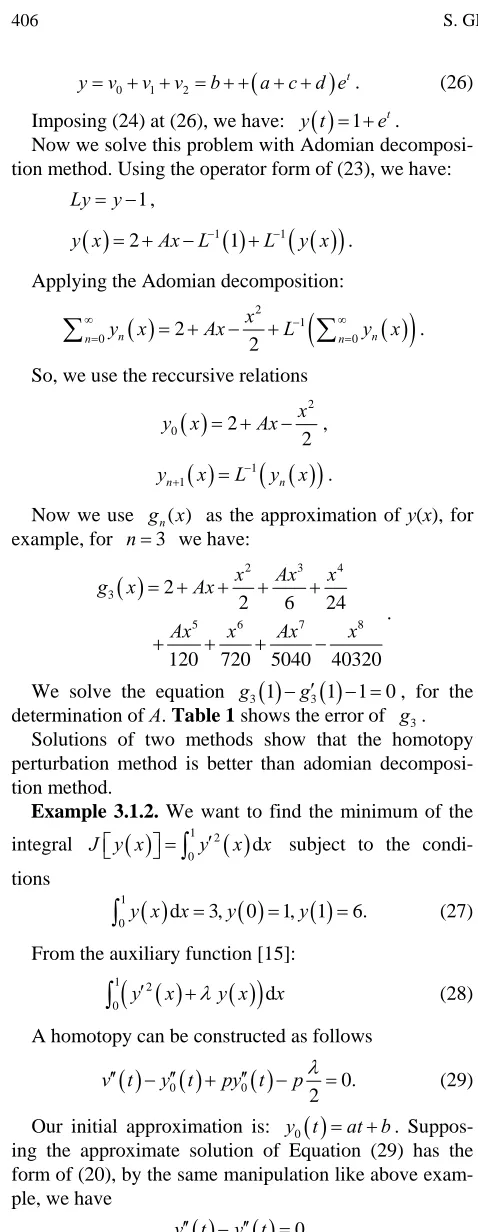
We solve the equation g3

 

1 g3

 

1  1 0, for the

determination of A. Table 1 shows the error of g3.

Solutions of two methods show that the homotopy perturbation method is better than adomian decomposi-tion method.

Example 3.1.2. We want to find the minimum of the integral

 

1 2

 

0 d

J y x_ _

_

y x x subject to the condi-tions

 

 

 

1

0y x xd 3,y 0 1,y 1 6



. (27) From the auxiliary function [15]:

 

 



1 ₂

0 y x  y x dx





(28) A homotopy can be constructed as follows

 

0

 

0

 

0.

2

v t y t py t p  (29) Our initial approximation is: y t0

 

atb.

Suppos-ing the approximate solution of Equation (29) has the form of (20), by the same manipulation like above exam-ple, we have

 

 

0 0 0

[image:4.595.51.290.52.668.2]

v t y t  ,

Table 1. Shows the error of g3.

x 0 0.2 0.4 0.6 0.8 1

e 0 0.203617e–3 0.415371e–3 0.643003e–3 0.889442e–3 0.113584e–2

 

 

1 0 0

2 v t y t   ,

 

2 0

v t  .

We suppose that v x0

 

y t0

 

ax b .

So

 

2

 

1 , 2 ,

4

v t t  ct d v t  et f 

Therefore we find the following equation

 

2



 

4

v x t  a c e t    b d f



(30) Imposing

 

 

1

 

0

0 1, 1 6, d 3

y  y 

_

y x x on (30) we

have:

 

2

12,y x 3x 2x 1

   

4. Combined Homotopy Perturbation

Method and Green’s Function Method for

Solving Second-Order Moving Boundary

Problems

Assume that [16]

 

2

 

   

 

, , 0

y x  y x f y x y x_  _F x  x l (32) with boundary conditions that obtained from transversal-ity conditions. Where  is a real constant number,



,



f y y is a nonlinear function, and F x

 

is a non-homogeneous term.

We can write Equation (32) to an equivalent integral equation;

 

1



 

   



 

0 , ,

y x  



F   f y_  y  _ G x d , (33) By adding a nonhomogeneous term, in moving boun- dary problems, the above equation is modified because boundary conditions are nonhomogeneous. Here, the function G x

 

, the function G x



,



that called Green’s function, is adjusted as below:

 

 









 









,

sin sin , 0

1

sin( ) sin sin , .

G x

l x x

l x l x l



  

     

  



 _

 



 

(34)

In Equation (33), if 0, then Green’s function amended as below:

 

1 ( ), 0

,

( ),

l x x

G x

.

x l x

l l

 



 

   

  _{  }

 (35)

We construct the homotopy form of Equation (33), which satisfies:



  

   

     

 

1 0 1

0

, , d

, , d 0,

H v p v x F G x

p f v v G x p

  

   

  

 _ _ 





 0,1 .

(36)

[image:4.595.55.282.78.297.2]

d power series of p as expressed in Equation (20) and

sub-stituting Equation (20) into (36) and equating the term with identical powers of p, The following equations can

be obtained:

 

1

   

0

0 ₀

: ,

p v x  

_

F  G x ,

 

1

 

 

 

 

 

   





1 2 0 1 2 0

0

: , , , , , , , , d ,

i

i i i i i

p v x  



f v   v   v  v  v   v  G x   i1, 2, 3,



We obtain the approximate solution from Equation (20) by solving these integral equation. If we construct the homotopy as:

 

1

  



1

0 , d , 4, 5, 6,

i i

v x  



v G x   i  . Assume that r x1

 

v x0

 

v x1





  

   





 

 

   





 

 

1 0 1 0

, , d

1 , ,

, d 0, 0,1 . exa exa

H v p v x F G x

p f y y pf v v

G x p

               _ _ _   





(37)



and by imposing boundary condition on that, we have:

1, 2, a b

so:

 

2 3 4

1

1 1 1

2 .

2 4 4

r x   x x x  x where yexa

 

x is the exact solution of (32), then we

have: And assuming r x2

 

v x0

 

v x1

 

v x2





and im-

posing boundary condition on that, we have:

 

   

 

   

1 0 ₀ 1 0 , d , , exa exa

v x F G x

f y y G x

   d        _ _





1, 2, a b

 (38) _so:

 

2 3 4 5

2

1 1 3 5 5 1

2

2 4 8 8 8 8

r x   x x  x  x  x  x

Equation (38) will give the exact solution. 6

.

Numerical Examples _{Also we can write:}

Example 4.1.1. Considering Ramsey growth model, we

have: 3

 

2 3 4

6 7 8

1 1 1 1 1

2

2 4 8 16 2

5 3 1

8 16 .

8

r x x x x x x

x x x

         5 d .

 

 

   

1 0 1 1 0 , d

, d 0

i

i

y x ax b G x

y G x

          





(39) _{But from (37) we have:}

Also we have:

 

1

 

0 2

0 ₀

1 1

: , d

2 2

p v x ax b 

_

G x ax b  x  x,

 

 





 





 

1 0 1 0

2 , d

1 ,

v x x G x

e pv G x

          





 

1

 

1

1 ₀ 0

2 3

1

: , d

2

,

1 1 1 1 1 1

2 2 4 2 2 4

p v x v G x bx

b a x a x x

          _   _ _  _     



So:

4

 

 





 

1 0 ₀ 1 0 2 ,

1 , d

1 2 x .

v x x G x

e G x x e xe

 d             





.

 

1

 

2

2 ₀ 1

2 3

4 5

: , d

1 1 1 1

4 2 4 8

1 1 3 1 3 1

4 2 8 4 8 8 ,

p v x v G x

bx b a x

b a x a x x

        _   _       _   _ _  _     



 

 

That is approach to exact solution. And also we obtain:

 

0, 1, 2, i

v x  i .

6

1 3

3 ₀ 2

4 5

6 7

1

: , d

8

3 1 1 3 3 1

8 4 16 8 8 4

1 3 3 1 1 1

8 8 8 8 4 16 ,

p v x v G x bx

b a x b a x

b a x a x x

         _   _  _          _   _ _  _     



The plot of v x r x r x r x0

       

,1 , 2 , 3 has been shown 3

8

  

in Figure 1.

Example 4.1.2. We want to solve Example 3.1.2 with this method. The Euler-Lagrange equation is:

0 2

y   .

0 0.2 0.4 0.6 0.5 1 r1 r2 r3

x 3

2.8

2.6

2.4

2.2

2

[image:6.595.117.487.83.321.2]

v0 (exact solution)

Figure 1. The plot of v0(x), r1(x), r2(x), r3(x) of Example 4.1.1.

 



_



_









1 ,

0

1 1

1 0

x l x

G x

l x x

l

x x

l

x x

 



 

 

 

 



  _{  }





  



  _{  }

 and

 

   

     

 

1 0 1 0

1 0

, d

, ,

, d , 2

y x ax b F G x

p f y y G x

ax b G x

  

d

  

 _{ }

  



 _ _

  









So

 

1

 

0

0 ₀

2

: ,

2 1

,

4 4

p v x ax b G x

x a x b



d  

 

  

 

 _  _ 

 



 

1

 

 

 

 

 

   





1 2 0 1 2 0

0

: , , , , , , , , d 0, 1, 2, 3,

i

i i i i i

p v x  



f v   v   v  v  v   v  G x    i 

by imposing boundary condition on that, we have:

 

2

5, 1, 12, 3 2 1

a b  y x  x  x .

5. Conclusion

In this paper, we solve the moving boundary and iso-perimetric problems by using Homotopy perturbation method. Embedding parameter p

 

0,1 can be taken into account as a perturbation parameter. By the applica-tion of Green’s funcapplica-tion, the problem concerned is trans-formed into an equivalent integral equation, which is solved using the homotopy perturbation method. Nu-merical examples show that these proposed methods were valid and effective for solving problems.

REFERENCES

[1] U. Brechtken-Manderschied, “Introduction to the Cal- culus of Variations,” Chapman Hall, London, 1991. [2] H. Sagan, “Introduction to the Calculus of Variations,”

Dover Publications, New York, 1992.

[3] J.-H. He, “A Coupling Method for a Homotopy Tech-nique and a Perturbation TechTech-nique for Nonlinear Prob-lems,” International Journal of Non-Linear Mechanics, Vol. 35, 2000, pp. 37-43.

[4] U. Ascher, M. Robert, M. M. Mattheij and R. D. Russell, “Numerical Solution of Boundary Value Problems for Ordinary Differential Equations,” SIAM, Philadelphia, 1995.

[5] G. Engstrom and U. Brechtken-Manderschied, “Introdu-

ction to the Calculus of Variations,” Chapman and Hall/CRC, London, 1991.

[6] D. D. Ganji, H. Tari and M. Bakhshi, “Variational Itera-tion Method and Homotopy PerturbaItera-tion Method for Nonlinear Evalution Equations,” Computers &

Mathe-matics with Applications, Vol. 54, No. 7-8, 2007, pp. 1018-1024.

[7] J. H. He, “Perturbation Method: A New Nonlinear Ana-lytical Technique,” Applied Mathematics and Computa-tion, Vol. 135, No. 1, 2003, pp. 73-79.

doi:10.1016/S0096-3003(01)00312-5

[8] M. Inokuti, H. Sekine and T. Mura, “General Use of the Lagrange Multiplier in Non-Linear Mathematical Phys-ics,” In: S. Nemat-Nassed, Ed., Variational Methods in the Mechanics of Solids, Pergamon Press, New York, 1978, pp. 156-162.

[9] S. J. Liao, “An Approximate Solution Technique Not De- pending on Small Parameters: A Special Example,”

In-ternational Journal of Non-Linear Mechanics, Vol. 30, No. 3, 1995, pp. 371-380.

doi:10.1016/0020-7462(94)00054-E

[10] S. J. Liao, “Boundary Element Method for General Non- linear Differential Operators,” Engineering Analysis with

Boundary Element, Vol. 20, No. 2, 1997, pp. 91-99.

doi:10.1016/S0955-7997(97)00043-X

[11] J. H. He, “Asymptotology by Homotopy Perturbation Method,” Applied Mathematics and Computation, Vol. 156, No. 3, 2004, pp. 591-596.

doi:10.1016/j.amc.2003.08.011

[13] R. Memarbashi, “Variational Problems with Moving Boundaries Using Decomposition Method,” Mathemati-cal Problems in Engineering, Vol. 2007, 2007, Article ID 10120. doi:10.1155/2007/10120

[14] J. H. He, “Homotopy Perturbation Method for Solving Boundary Value Problems,” Physics Letters A, Vol. 350, No. 1-2, 2006, pp. 87-88.

[15] M. L. Krasnov, G. I. Makarenko and A. L. Kiselev,

“Problems and Exercises in the Calculus of Variations,” George Yankovsky, Moscow, 1975.

[16] Y.-G. Wang, H.-F. Song and D. Li, “Solving Two-Point Boundary Value Problems Using Combined Homotopy Perturbation Method and Green’s Function Method,”