Gliding flight: speed and acceleration of ideal falcons during diving and pull out

Many birds of prey attack from a high-speed dive: a fixed-wing glide along a steep, straight path. This behavior is particularly characteristic of peregrines (Falco peregrinus), falcons that strike other birds in the air, often after a spectacular dive that begins hundreds of meters above the prey (Cade, 1982). Prior to a dive, a peregrine typically accelerates by beating its wings, and then begins the dive by folding its wings and steepening its flight path to an angle that ranges from approximately 15 ° from horizontal to near vertical. The bird accelerates during the dive at the expense of potential energy and may reach what are thought to be the highest speeds attained by animals – estimates of top speeds range up to 157 m s−1 (351 miles h−1) (Brown, 1976; Clark, 1995; Dement’ev, 1951; Hantge, 1968; Lawson, 1930; Mebs, 1975; Orton, 1975; Savage, 1992; Tucker and Parrott, 1970).

While these estimates may be correct, their accuracy is unknown because the speed of a diving falcon is difficult to measure. The required instrumentation is complex, and the dive is a brief, rare event that takes place at unpredictable places and times, usually at a long distance from the observer. Alerstam (1987) used radar to overcome these difficulties, and he measured diving speeds of no more than 39 m s−1 in a peregrine. Clark (1995) doubts that diving speeds exceed 41 m s−1.

The speeds reached in a dive are constrained by the aerodynamic properties of the bird, the angle of the dive, the acceleration of gravity and the space and time available for acceleration; and an analysis of these variables can set the limits of which falcons are capable. Several mathematical models for gliding flight are available (Pennycuick, 1971a, Printed in Great Britain © The Company of Biologists Limited 1998

JEB1074

Some falcons, such as peregrines (Falco peregrinus), attack their prey in the air at the end of high-speed dives and are thought to be the fastest of animals. Estimates of their top speed in a dive range up to 157 m s−1, although speeds this high have never been accurately measured. This study investigates the aerodynamic and gravitational forces on ‘ideal falcons’ and uses a mathematical model to calculate speed and acceleration during diving. Ideal falcons have body masses of 0.5–2.0 kg and morphological and aerodynamic properties based on those measured for real falcons.

The top speeds reached during a dive depend on the mass of the bird and the angle and duration of the dive. Given enough time, ideal falcons can reach top speeds of 89–112 m s−1 in a vertical dive, the higher speed for the heaviest bird, when the parasite drag coefficient has a value of 0.18. This value was measured for low-speed flight, and it could plausibly decline to 0.07 at high speeds. Top speeds then would be 138–174 m s−1.

An ideal falcon diving at angles between 15 and 90 ° with a mass of 1 kg reaches 95 % of top speed after travelling approximately 1200 m. The time and altitude loss to reach 95 % of top speed range from 38 s and 322 m at 15 ° to 16 s and 1140 m at 90 °, respectively.

During pull out at top speed from a vertical dive, the 1 kg ideal falcon can generate a lift force 18 times its own weight by reducing its wing span, compared with a lift force of 1.7 times its weight at full wing span. The falcon loses 60 m of altitude while pulling out of the dive, and lift and loss of altitude both decrease as the angle of the dive decreases.

The 1 kg falcon can slow down in a dive by increasing its parasite drag and the angle of attack of its wings. Both lift and drag increase with angle of attack, but the falcon can cancel the increased lift by holding its wings in a cupped position so that part of the lift is directed laterally. The increased drag of wings producing maximum lift is great enough to decelerate the falcon at −1.5 times the acceleration of gravity at a dive angle of 45 ° and a speed of 41 m s−1(0.5 times top speed).

Real falcons can control their speeds in a dive by changing their drag and by choosing the length of the dive. They would encounter both advantages and disadvantages by diving at the top speeds of ideal falcons, and whether they achieve those speeds remains to be investigated.

Key words: peregrine falcon, Falco peregrinus, bird, flight, diving, mathematical modelling, acceleration, speed.

Summary

Introduction

GLIDING FLIGHT: SPEED AND ACCELERATION OF IDEAL FALCONS DURING

DIVING AND PULL OUT

VANCE A. TUCKER

Department of Zoology, Duke University, Durham, NC 27708, USA

1975, 1989; Tucker, 1987), and Alerstam (1987) modified one of them for diving flight. None of the models, however, accounts for acceleration during the dive or during the subsequent pull out.

This paper introduces a mathematical model for the diving performance of mathematically defined ‘ideal falcons’, named after the useful ‘ideal gas’ of physical chemistry. Ideal falcons have a range of body masses, morphological characteristics and aerodynamic properties that are similar to those of their real counterparts, and the model answers the following questions about them. How fast can they go in a dive? How much time and altitude do they need to accelerate? What effects does the angle of the dive have on acceleration? How much aerodynamic force can they produce to pull out of a dive, and how much altitude do they lose in the pull out? How much can they control their speed in a dive?

The answers to these questions provide a framework for evaluating the diving performance of real falcons in nature, but they do not necessarily describe real falcons. The aerodynamic forces on ideal falcons are extrapolations based on measurements at speeds less than one-fifth of those that ideal falcons can achieve, and ideal falcons may assume shapes for which no measurements on a real bird exist. Ideal falcons have the over-riding virtue that they are products of mathematical relationships that can be examined, tested and modified as new experimental data accumulate.

Types of gliding

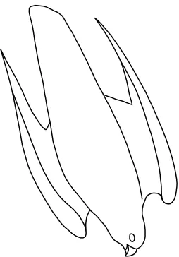
Gliding birds hold their wings at a range of spans, depending on speed. At low speeds, they spread their wings fully and they progressively reduce their wing span as speed increases. In steep, high-speed dives, they may hold their wings almost as close to the body as they do while perched (Fig. 1). The present study uses wing span to distinguish diving from two other types of gliding: soaring and flex gliding.

‘Soaring’ is often defined as a process in which a bird maintains or gains altitude by flying in air that is moving upwards or accelerating although, in the ornithological literature, the term describes a bird with near-maximum wing span and a spread tail. For example, gliding birds often gain altitude in a thermal by circling slowly with their wings at 90 % or more of full span. To achieve these spans, they swing their wings forwards and spread their tails to counteract the resulting pitching moment. This behavior can be seen in birds gliding in nature, and Tucker (1992) investigated it in a Harris’ hawk (Parabuteo unicinctus) trained to glide in a wind tunnel.

At speeds higher than those for soaring (in the ornithological sense), the tail folds and, over a range of speeds, a bird can glide along a path inclined at a minimum angle to the horizontal. The wings flex and wing span decreases to approximately 70 % of maximum at the high-speed end of this range (Tucker and Parrott, 1970; Tucker and Heine, 1990), where the bird is ‘flex gliding.’ Birds of prey typically flex glide when they glide off at high speed in a constant direction after gaining altitude by circling in thermals while soaring.

Birds can glide faster still by steepening the glide path and flexing their wings even more until, at some point, they are diving. For want of a convention that identifies the onset of diving, I shall describe a bird as diving when its wing span is less than 70 % of maximum and its glide path is straight. A bird pulling out of a dive is not diving, even though its wing span may be less than 70 % of maximum, because it does not follow a straight glide path.

Morphology and aerodynamic characteristics of ideal falcons

Morphological characteristics and the glide path

Ideal falcons (or simply ‘falcons’ to distinguish them from real falcons) have mass m and are bilaterally symmetrical. They have a long axis that extends from the tip of the beak to the tip of the tail in the plane of symmetry, and planes perpendicular to the long axis cut a falcon’s body into cross sections that vary in area and width along the long axis. The area of the cross section with the maximum area (exclusive of the wings) is Sb, and the width of the cross section with the

maximum width (including the wings) is the wing span b. A falcon with a given mass has a fixed value of Sbbut can adjust

its wing span between maximum and minimum values (bmax

and bmin).

As the wing span varies, the surface area of the wings (Sw)

also varies between maximum and minimum values (Sw,max

and Sw,min). Swis the projected area of the wings on the plane

that is perpendicular to the plane of symmetry and contains the long axis. Wing area includes the projected area of the bird’s body between the wings.

With one exception, the wings of falcons have no dihedral; i.e. the chord lines of the wings intersect the plane for the projected area of the wings. A chord line is the line between the leading and trailing edges of a wing section cut by a plane parallel to the plane of symmetry. The lengths of the chord lines vary along the wing span, and the mean length is the chord (c):

c = Sw,max/bmax. (1)

The exception is that ideal falcons, like real falcons (Fig. 1), may cup their wings around the body (see Fig. 6). The bottom surfaces of the cupped wings face the sides of the body, as when perched, but with a space between the wings and the body. The present paper refers to cupped wings only in the discussion of the control of diving speeds.

As a falcon glides, a position vector (P) traces out its glide path through space as time (t) passes. A position in space is a point on orthogonal x,y coordinates, since space is two-dimensional in this study. The falcon moves along the glide path at velocity dP/dt=V, a vector with components Vxand Vy,

and the glide path while diving is a straight line inclined at an angle (θ) to the horizontal x axis.

There is no wind, so a diving falcon glides in an inertial frame of reference at air speed V and may accelerate by changing speed but not direction. During the pull out from a dive, the falcon accelerates by changing direction but not speed.

The present paper uses the common convention of defining

y as a loss in altitude, and orienting the x and y axes with values

on the y axis increasing in a downward direction. x values increase towards the right, and θincreases as the glide path rotates in a clockwise direction (Fig. 2).

Aerodynamic and gravitational forces and shape

A gliding falcon experiences two types of force: a constant gravitational force (weight) and a variable aerodynamic force generated by the air flowing over the body and wings. Weight is directed vertically downwards and has magnitude W equal to mg, where m is body mass and g is the magnitude of gravitational acceleration (9.81 m s−2_{in this study). Weight has}

components that are parallel and perpendicular to the glide path: Wsinθand Wcosθ, respectively (Fig. 2).

The aerodynamic force has a magnitude and direction that varies with V and the shape of the bird’s body – in particular, with the angle of attack of the wing. The angle of attack is the angle between a chord line and the projection of the glide path on the vertical plane that contains the chord line.

Since a diving falcon follows a straight glide path, it has no acceleration in a direction perpendicular to the glide path, and the perpendicular component of the aerodynamic force must sum to zero with the perpendicular component of the gravitational force. In contrast, the parallel components of the aerodynamic and gravitational forces may not sum to zero, in which case the falcon accelerates along the glide path.

The perpendicular and parallel aerodynamic components multiplied by −1 are lift (L) and drag (D), respectively. Therefore, during diving:

L = Wcosθ, (2)

dV/dt = gsinθ −D/m . (3) When drag equals the parallel weight component, the falcon is at equilibrium and moves along the glide path at constant speed

Ve. Otherwise, it is not at equilibrium and accelerates.

The term ‘shape’ refers to any dimension or orientation of the falcon that influences the aerodynamic force at a given

speed. For example, birds can change their drag by changing the angle of attack of the wings, the wing span and the position of the feet (Pennycuick, 1971b; Tucker, 1987, 1988). They may also change drag by cupping their wings or by changing the orientation of their long axis relative to the glide path. A ‘shape factor’ is a shape feature that has been defined as a quantity, such as wing span or angle of attack.

Performance and velocity polar diagrams

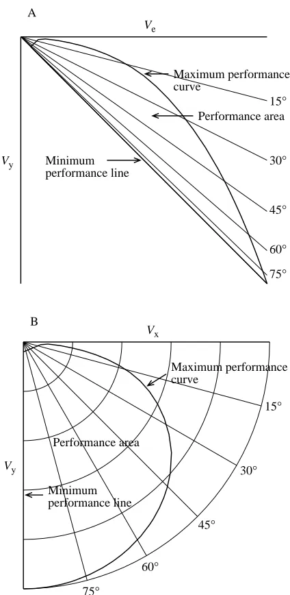
The performance diagram (Fig. 3A) shows Vy plotted

against Ve, and is the conventional way of describing the

equilibrium gliding performance of birds. This study uses a transformation of the performance diagram – the velocity polar diagram – to describe both equilibrium and non-equilibrium diving in falcons, and I shall summarize the features of the performance diagram (see Tucker, 1987, 1988, for a complete analysis) as an introduction to the velocity polar diagram.

The relationship between Vyand Vedepends on drag since,

at equilibrium:

D = Wsinθ, (4)

and

sinθ= Vy/Ve. (5)

Therefore,

Vy= DVe/W . (6)

For many manufactured gliders, drag is a single-valued

Fig. 2. Gravitational and aerodynamic force vectors (bold lines) and their components for a bird gliding to the right on a glide path inclined

at angle θto the horizontal. The gravitational vector has magnitude

W and a component Wcosθthat is balanced by the lift component (L) of the aerodynamic force, which has magnitude F and a direction

given by angle ϕ. The drag component (D) of the aerodynamic force

does not balance the gravitational component Wsinθ, so the bird

accelerates to the right.

Glide path

ϕ

θ

Wsinθ

Wcosθ

y

x

W

L F

D

function of Ve in normal, straight-line flight, and the

performance diagram is simply a curved line, also known as the ‘glide polar’ (Pennycuick, 1989). Gliding birds, however, can have a range of drag (and θ) values for a given Ve, because

they can change their shape – particularly their wing span. As a result, their performance diagrams are areas bounded by two curves: the maximum performance curve (or ‘superpolar’; Pennycuick, 1989) and the minimum performance line, the area enclosed by these lines being the performance area. A bird gliding at a given Ve has minimum drag when θ is at a

minimum, in which case the bird has equilibrium speed at

maximum performance, and Ve=VE. The maximum

performance curve shows Vy plotted against VE, and the

minimum performance line describes birds in vertical dives; i.e. Vy=Ve, drag is maximum for each Ve and drag equals

weight. The straight lines through the origin in Fig. 3A indicate different directions of the glide path.

The velocity polar diagram (Fig. 3B) contains the same information as the performance diagram, but shows Vyplotted

against Vx, rather than Ve. Vxand Vyare the components of the

velocity vector V, which can be visualized on the polar diagram as the resultant of the two components. VEfrom θ =

some minimum glide angle to 90 ° describes the maximum performance curve, and the minimum performance line lies along the Vyaxis. The performance area between the maximum

performance curve and the Vyaxis is greatly expanded at large

values of θ, compared with the performance diagram (Fig. 3A). Straight lines through the origin in Fig. 3B indicate different directions of the glide path, and constant values of V appear as circular arcs when Vxand Vyhave the same scale.

In this study, the velocity polar diagram describes both equilibrium and non-equilibrium gliding. At given values of θ and t, the bird may be accelerating at speed V or may be at equilibrium if drag equals Wsinθ. At equilibrium, the bird’s speed is either Ve, if less than the maximum for that value of

θ, or VE, if at the maximum.

One can envision a bird on the polar diagram moving slowly at the beginning of its dive along a glide path that has the same direction as the vector V. As the bird accelerates, its drag increases until drag is equal to Wsinθ, and then speed is constant at either Veor VE, depending on body shape.

The mathematical model

The mathematical model describes equilibrium gliding and two types of non-equilibrium gliding: diving, during which θ is constant and speed varies, and the pull out from a dive, during which speed is constant and θvaries. The part of the model for equilibrium gliding is taken from Tucker (1987), and the parts for non-equilibrium gliding are new. The next section summarizes the model for equilibrium gliding at maximum performance and establishes the relationships used in the analysis of non-equilibrium diving and the pull out from the dive.

Equilibrium gliding at maximum performance

For a bird to glide at maximum performance (and speed VE),

it must shape itself to meet two constraints: the wings must produce lift equal to Wcosθ, and the body and wings must have minimum drag at VE. Tucker (1987, 1988) analyzed the

variables that influence shape, lift and drag at VEvalues of less

than 30 m s−1_{, and this paper extends that analysis to higher and}

non-equilibrium speeds. The summary below introduces the variables and the relationships between them that are relevant to this study.

Dynamic pressure (q) appears repeatedly in the equations for lift and drag:

V_e

Vy

Maximum performance curve

Performance area

Minimum performance line

15°

30°

45°

60°

75°

A

V_x

Vy

Maximum performance curve

Performance area

Minimum performance line

15°

30°

45°

60°

75°

B

Fig. 3. A performance diagram (A) and a velocity polar diagram (B) for a gliding bird. Both diagrams show the same information, but plot different quantities on the horizontal axes. The thin lines show the

direction of the glide path for different glide path angles θ. See text

for an explanation of the maximum performance curve, the minimum

performance line and the performance area. Ve, equilibrium speed; Vx,

horizontal component of velocity through the air; Vy, vertical

q = 0.5ρV2_{, (7)}

where the density of air (ρ) is equal to 1.23 kg m−3 _{in this}

study – the value for the standard atmosphere at sea level at a temperature of 15 °C (von Mises, 1959).

Reynolds number (Re) influences the drag coefficients (defined below) on which drag depends:

Re =ρdV/µ, (8)

where d is a specified distance dimension on the falcon and µ is the viscosity of air. In the standard atmosphere described above for ρ, µ=17.8×10−6_{kg m}−1_s−1. ρ, d, µ_{and the turbulence}

of the air are all constant for a falcon in this study, and drag coefficients are functions only of V and a falcon’s shape.

The lift component L, together with Swand q, define the lift

coefficient CL:

CL= L/(qSw) , (9)

which, in turn, determines the profile drag coefficient (discussed below). In a dive at a given angle, the only shape factor that influences CLis the wing span, since L is constant

(equation 2) and Swvaries with wing span.

Drag is the sum of three terms: induced drag, which results from lift production; profile drag, which is the drag of the wings minus the induced drag; and parasite drag, which results from the body exclusive of the wings.

The shape factor for induced drag (Di) is wing span:

Di= 1.1L2/(πqb2) . (10)

The shape factor for profile drag (Dpr) is also wing span:

Dpr= qSwCD,pr, (11)

because the profile drag coefficient (CD,pr) is a function of CL

and, therefore, of b. CD,pr is also a function of Re when the

distance variable for Re is the chord, c (Tucker, 1987). The shape factor for parasite drag (Dpar) is the

cross-sectional area (Sb) of the body:

Dpar= qSbCD,par, (12)

and Sband the parasite drag coefficient CD,parare constants for

a falcon of a given mass. CD,pardepends on the position of the

feet and tail and the alignment of the long axis of the body with the glide path. Ideal falcons control their shapes to minimize

CD,parwhen gliding at maximum performance.

CD,paralso depends on Re. It declines with increasing Re in

various manufactured bodies and probably does so in real birds. For example, Prandtl and Tietjens (1957, p. 101) report a decline in CD,parof more than half for a birdlike body over

a range of Re that applies to falcons. Although the model keeps

CD,parconstant as Re changes, this study gives some examples

of the effects of low CD,parvalues on diving performance.

Drag D is the sum of equations 10, 11 and 12 and, at a given speed, is a function of b that has a minimum (Dmin) at span b0.

For example, if a falcon increases its wing span, induced drag decreases, but profile drag increases owing to the increase in

Sw. However, the increase in Swdecreases CLwhich, in turn,

decreases CD,pr and mitigates the increase in profile drag.

Taken together, these changes result in minimum drag when falcons hold their wings at maximum span at slow speeds and flex their wings to decrease wing span as speed increases, just as real falcons do in nature and in a wind tunnel (Tucker and Parrott, 1970).

The mathematical model finds maximum performance curves for ideal falcons by setting the partial derivative ∂D/∂b

to 0, and finding Dminand b0. Both are functions (f) of V:

Dmin= f1(V) , (13)

b0= f2(V) , (14)

with the provision that b0may not exceed bmax. Tucker (1987)

describes these functions and an iterative procedure for finding maximum performance curves for gliding birds, and Thomas (1996) uses a similar procedure for finding the minimum power required for flapping flight.

Non-equilibrium gliding Diving

During non-equilibrium diving, a falcon accelerates along a straight glide path inclined at angle θ to the horizontal and adjusts its wing span and CD,parto keep drag to a minimum at

each speed. From equations 3 and 13,

dV/dt = gsinθ −f1(V)/m . (15)

The solution to this differential equation can be found by numerical methods and gives the speed of the falcon as time varies:

V = f3(t) . (16)

At each speed, b0has a particular value, and the relationship

between b0and V:

b0= f4(V) , (17)

can be found by combining equations 14 and 16. The distance (s) that the falcon travels as time varies can be found by numerical integration of equation 16, and the falcon’s loss of altitude (y) is:

y = ssinθ. (18)

The functions f1–f4depend on mass-related characteristics of

ideal falcons, described in a later section. A computer program for the calculations is available from the author.

Pull out from a dive

Ideal falcons pull out of a dive by gliding at constant speed along a circular arc until the glide path is horizontal. These characteristics simplify the analysis of the pull out, but they prescribe an altitude drop (∆y) during the pull out that is

probably greater than that required by real falcons. Real falcons decrease their speed during pull out, and they need not follow a circular path. Both factors reduce ∆y, but an analysis of them

is beyond the scope of this study.

is the difference between lift and the gravitational force component Wcosθ. Therefore:

r = mV2_/(L

1−W) , (19)

since the denominator is constant and L=L1 when θ=0. In

addition, L1is the maximum lift that the falcon can produce at

speed V, because the falcon minimizes ∆y, and therefore r,

during pull out.

∆y depends on the angle (θ0) of the glide path at the

beginning of the arc. From Fig. 4:

∆y = r(1−cosθ0) . (20)

Combining equations 19 and 20: ∆y = mV2₍₁−cosθ

0)/(L1−W) . (21)

At first glance, one might think that the falcon could achieve maximum lift during pull out by maximizing CL, wing span

and wing area, as it does at low speeds. However, at high speeds, the lift on the wings in this configuration would generate intolerable torque around the shoulder joints. The falcon can reduce this torque by flexing its wings to a shorter span with less wing area, thereby reducing both the moment arm for the torque and the lift on the wings. At some span, the torque is the maximum tolerable when the lift is maximum for the wing area associated with that span, and L=L1. The

following analysis shows how to find L1 and compute the

minimum value of ∆y needed for a pull out.

In ideal falcons, the center of lift on one wing is at a point midway between the wing tip and the shoulder joint. Therefore, the moment arm for the torque around the shoulder joint when the wings have maximum span is (bmax−bmin)/4. The maximum

torque that the falcon can tolerate with maximum wing span is

L0(bmax−bmin)/8, where L0/2 is the maximum lift on one wing.

At spans less than bmax, the moment arm for the torque on one

wing is (b−bmin)/4, and the lift (LT) from both wings at

maximum torque is:

LT= L0(bmax−bmin)/(b−bmin). (22)

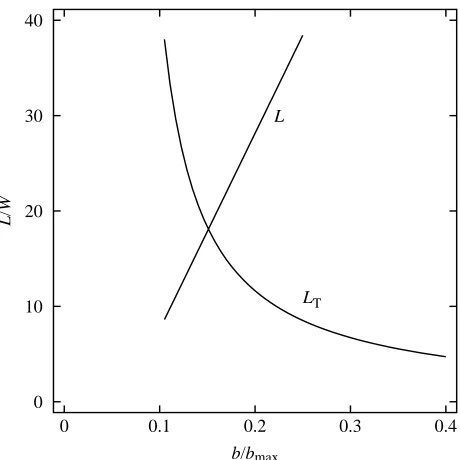
However, the wings at short spans may not have enough area to produce LT, since the maximum lift that they can produce is:

L = 1.6qSw, (23)

where 1.6 is the maximum value of CL for ideal falcons. At

some span (b1), the maximum lift that the wings can produce

equals LT(Fig. 5), in which case, L=L1. b1may be found by

equating LT and L, substituting for Sw from equation 25 and

rearranging:

b1= (bmax−bmin) [L0/(1.6qSw,max)]1/2+ bmin. (24)

Substituting b1for b in equation 22 yields L1=LT; and with L1

in hand, ∆y can be calculated from equation 21.

Control of speed in a dive

An ideal falcon controls its speed in a dive by increasing drag by various means (see above). This section considers only an increase in drag generated by the wings; i.e. profile and induced drag.

The falcon can increase these two types of drag at a given speed by increasing the angle of attack of the wings, but a problem arises: an increase in the angle of attack of an unstalled wing also increases lift, yet lift must remain constant at a given dive angle (equation 2). The falcon overcomes this constraint by cupping its wings so that the projection of each wing on the plane of symmetry has substantial area. As a result, each wing produces an aerodynamic force component that is perpendicular to drag and has a lateral component (Fig. 6). During vector addition, the lateral components cancel, and the falcon can increase both angle of attack and drag with no change in L.

Pull out path Dive path

θ0

θ0 θ

∆y

y

x

r

r

Fig. 4. The arc followed by an ideal falcon pulling out of a dive from

a dive path inclined at angle θ0. During the pull out, θdeclines from

θ0to 0, and the falcon loses altitude ∆y while remaining a constant

distance r from the center of the arc.

0 0.1 0.2 0.3 0.4

0 10 20 30 40

b/bmax

L

/W

L

L_T

Fig. 5. Dimensionless lift for maximum torque (LT) and lift (L) for

maximum CLat different dimensionless wing spans b/bmaxfor a 1 kg

ideal falcon at a speed of 100 m s−1_{. The wings can produce lift with}

tolerable torque only in the region that is beneath both curves, and the

Not enough is known to allow accurate calculation of the drag of falcons with cupped wings but, for heuristic purposes, I shall use the equations for drag already given and allow CL

to have any value up to its maximum. If the chosen CLresults

in more lift than that specified in equation 2, the extra lift is understood to be lateral components that cancel.

Mass-related characteristics of ideal falcons Ideal falcons are geometrically similar in shape and have body masses between 0.5 and 2.0 kg, corresponding to a small, male peregrine and a large, female gyrfalcon (Falco

rusticolus), respectively. Given the body mass of an ideal

falcon, all of the aerodynamic characteristics that influence gliding performance in this study can be calculated from several constants (Table 1) derived from aerodynamic measurements on two real falcons: a laggar (Falco jugger) (body mass 0.570 kg) (Tucker and Parrott, 1970) and a peregrine (body mass 0.713 kg) (Tucker, 1990).

Wing area varies linearly with wing span:

Sw= Sw,max(b−bmin)/(bmax−bmin) . (25)

This relationship is similar to those measured in real hawks (Tucker and Heine, 1990; Tucker and Parrott, 1970). The smallest wing span that a falcon can have in flight is 0.1bmax,

which is larger than bmin.

The lift and profile drag coefficients of a manufactured wing of fixed span are related as angle of attack varies, and Tucker (1987) showed that there is also a relationship between these coefficients in birds gliding at minimum angles with a range of speeds and wing spans. The relationship depends on Sband CD,par, since calculation of CD,pr involves subtraction of

parasite drag from total drag. For ideal falcons:

CD,pr= 0.0512−0.084CL+ 0.0792CL2 (26)

for values of CL between 0.53 and 1.65 at Re=105, based on d=c. CD,prdoes not change when CLdecreases below 0.53 at

a given value of Re. Equation 26 is derived from data for the laggar (Tucker, 1987), with Sband CD,parfrom Table 1.

CD,pr varies with Re in ideal falcons, and Tucker (1987)

shows how to calculate CD,prat Re values other than 105. Re

affects CD,pronly up to an Re value of 5×105and has no effect

at higher values.

Ideal falcons can produce a maximum lift L0 of 1.7W at

maximum wing span, in which case the torque around the shoulder joint is the maximum tolerable. This value for L0

comes from measurements of the maximum weight that Harris’ hawks could carry at slow speed (an estimated 10 m s−1₎

(Pennycuick et al. 1989), and it is also consistent with the maximum weight-carrying abilities at take-off of other birds that have 25 % of their body mass made up of flight muscles (Marden, 1987, 1990).

Diving performance of ideal falcons

The questions about diving posed in the Introduction can now be answered for ideal falcons, and this section answers them for selected sets of variables. First, it shows the effects of body mass by describing the diving performance of a large and small falcon at the ends of the mass range, and then it shows the effects of glide angles of 15, 30, 45 and 90 ° on the performance of a falcon with a mass comparable to that of a large peregrine, 1 kg. It also describes pull out from dives and the effects of cupped wings on acceleration during a dive.

The effect of body mass

During equilibrium gliding at VE, wing span declines rapidly

with speed for both the large and small falcons (Fig. 7). Diving commences at speeds of 15–20 m s−1_{, when wing span drops}

below 0.7bmax.

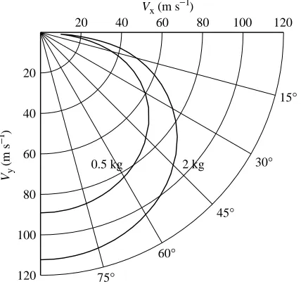
The larger falcon has a higher VEthan the smaller one at a

given value of θ (Fig. 8). For both birds, VE is high during

diving even at small values of θ. VE=Vmaxat θ=90 °, but even

in a shallow dive when θ=20 °, VEis greater than 0.5Vmax; by

θ=45 °, VEis greater than 0.8Vmax.

The Vmaxvalues in Fig. 8 are very high by the standards of

terrestrial animals. The larger falcon can reach speeds more than three times higher than the fastest running animal. Few wheeled vehicles can reach speeds of 100 m s−1_{, nor can many}

light, propeller-driven airplanes in level flight.

The values for VEin Fig. 8 are conservative, because they are Fig. 6. A head-on view of a falcon with cupped wings. The arrows

show the directions of force components on unit areas of the wings at certain points. The vector sum of all of these components over the wing area is lift.

Table 1. Mass-related characteristics of ideal falcons

Q C K Base datum

bmax 1.218 m kg−1/3 1/3 1.01 m*

bmin 0.0844 m kg−1/3 1/3 0.07 m**

Sw,max 0.192 m2kg−2/3 2/3 0.132 m2*

Sb 0.00838 m2kg−2/3 2/3 0.00669 m2***

CD,par 0.18 0 0.18***

L0 1.7g 1 See text

*Falco jugger; **Falco jugger, width between the shoulder joints; ***Falco peregrinus.

A mass-related characteristic Q may be calculated from the

constants C and K with the equation Q=C mK_.

m, mass; bmax, maximum wing span; bmin, minimum wing span; Sw,max, maximum wing area; Sb, maximum cross-sectional area of

body; CD,par, parasite drag coefficient; L0, maximum lift at maximum

based on a value of 0.18 for CD,parthat does not change with Re.

If CD,parwere to drop to 0.07 as Re increases, as it does for some

manufactured objects (see section on parasite drag), Vmaxwould

be 138 and 174 m s−1_{for the small and large falcons, respectively.}

During non-equilibrium diving, the large and small falcons accelerate along a glide path inclined at 45 °. The curves (Figs 9, 10) that illustrate non-equilibrium diving end at the time taken to accelerate from 15 m s−1 _{to 0.95V}

E, since V

approaches VEasymptotically.

The large and small falcons take 18 s and 23 s to accelerate from 15 m s−1 _{to 0.95V}

E, and drop 679 m and 1078 m while

doing so. These times and distances are surprisingly large and suggest that real falcons in most circumstances will seldom be seen diving at speeds close to VE. If starting the dive in the air,

they would be at such high altitudes that they would be difficult

0 20 40 60 80 100 120

0 0.2 0.4 0.6 0.8 1.0

Speed, V_E (m s−1)

b

/bmax

2 kg

0.5 kg

Vx (m s−1)

20 40 60 80 100 120

Vy

(m s

−

1 )

20

40

60

80

100

120

2 kg 0.5 kg

15°

30°

45°

60°

75°

Fig. 7. Dimensionless wing spans b/bmax of ideal falcons with masses

of 0.5 and 2.0 kg, gliding at equilibrium at different speeds VEalong

maximum performance curves.

Fig. 8. The maximum performance curves and minimum performance lines in a velocity polar diagram for ideal falcons with masses of 0.5

and 2.0 kg. Vx, Vy, horizontal and vertical components of velocity,

respectively; see also Fig. 3B.

Fig. 9. The speed (V) at different times (t) for ideal falcons that dive

at an angle θ of 45 ° and reach 95 % of the equilibrium speed VEfor

this angle. The falcons have masses of 0.5 and 2 kg, and begin their

dives at a speed of 15 m s−1_.

Fig. 10. The loss in altitude (y) at different times for ideal falcons that

dive at an angle θof 45 ° and reach 95 % of the equilibrium speed VE

for this angle. The falcons have masses of 0.5 and 2 kg, and begin

their dives at a speed of 15 m s−1_.

0 5 10 15 20 25

0 20 40 60 80 100

Time, t (s)

Speed,

V

(m s

−

1 )

2 kg

0.5 kg

0 5 10 15 20 25

1200 1000 800 600 400 200 0

Time, t (s)

Altitude loss,

y (m)

0.5 kg

to see with the unaided eye. If perched, they would have to be on a mountain or a cliff, as the world’s tallest structure (an antenna tower) is only 623 m high (Crystal, 1997). An observer could expect to see only part of the dive at close range, since the distance traveled during the dive is long, 1.4 times the drop in altitude for a 45 ° dive.

Effect of dive angle

This section describes the effect of dive angle on acceleration during diving by a 1 kg falcon. As the glide angle steepens, the falcon accelerates faster from 15 m s−1_{to 0.95V}

E

(Fig. 11), and the vertical drop also increases (Fig. 12). The total distance traveled while accelerating to 0.95VEis

nearly independent of dive angle – within 6 % of the mean value of 1211 m. That is, if the falcon intends to reach its prey at 0.95VE, it must start the dive at approximately 1200 m from

the prey, no matter what the dive angle. If the parasite drag coefficient were 0.07 rather than 0.18, the mean distance traveled would increase nearly 2.5-fold to 2964 m.

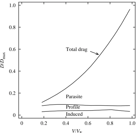
Almost all of the drag at VEis parasite drag (Fig. 13). For

example, at the start of a 45 ° dive by a 1 kg falcon, approximately one-quarter of the drag is parasite drag. As the bird accelerates, this proportion increases to approximately 90 %, while profile and parasite drag remain nearly constant.

The pull out from a dive

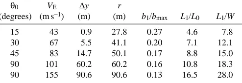
Table 2 shows the performance of the 1 kg ideal falcon pulling out of dives at VE at various angles. The falcon achieves

remarkably high values of lift with flexed wings – more than an order of magnitude above its maximum lift with maximum wing

span. The acceleration during pull out may also be high – more than an order of magnitude above that of gravity (g). The ratio of acceleration to gravitational acceleration is the ratio of L1to W, minus 1.

0 10 20 30 40

0 20 40 60 80 100

Time, t (s)

Speed,

V

(m s

−

1 )

15°

30°

45°

90°

0 10 20 30 40

1200 1000 800 600 400 200 0

Time, t (s)

Altitude loss,

y (m)

15°

30°

45°

90°

Fig. 11. The speed (V) at different times (t) for an ideal falcon diving

at different inclinations θand reaching 95 % of the equilibrium speed

VEfor each angle. The falcon has a mass of 1.0 kg and begins the

dives at a speed of 15 m s−1_.

Fig. 12. The loss in altitude (y) at different times for an ideal falcon

diving at different inclinations θand reaching 95 % of the equilibrium

speed VEfor each angle. The falcon has a mass of 1.0 kg and begins

the dives at a speed of 15 m s−1_.

0 0.2 0.4 0.6 0.8 1.0

0 0.2 0.4 0.6 0.8 1.0

V/V_E

D

/D

max

Induced Profile Parasite Total drag

Fig. 13. Dimensionless drag (D/Dmax) at different dimensionless

speeds (V/VE) for a 1 kg ideal falcon accelerating along a glide path

inclined at 45 ° to the horizontal. Three components of total drag (induced, profile and parasite) are plotted cumulatively so that they

add up to total drag. VEis 82.9 m s−1and total drag (Dmax) at this speed

Control of speed in a dive

Ideal falcons with cupped wings can hold their speeds constant or even decelerate strongly, merely by adjusting the angle of attack of the wings. For example, the 1 kg falcon, diving at an angle of 45 ° at a speed of 0.5VE(41 m s−1) with

minimum drag, is accelerating; and it could stop accelerating by increasing drag to Wsinθ. It could achieve this drag solely by increasing its lift coefficient to 0.77 and extending its wings to a span of 0.37bmax, a value that generates the maximum

tolerable torque around the shoulder joints (equation 24). The falcon could decelerate (negative acceleration) at −1.5g by increasing CLto 1.6 and reducing its wing span to 0.28bmax

to keep torque at the maximum tolerable level. This is a large deceleration by human standards, not reached during even violent maneuvers in automobiles. Automobiles on a level road can generate maximum accelerations that are equal to the frictional coefficient between the tires and the road when acceleration is expressed as a multiple of g. For example, the maximum deceleration during braking on a high-friction road is −0.8g (Limpert, 1992); and a deceleration of −1g feels like sitting, restrained by seat belts, in an automobile hanging vertically from its rear bumper.

Discussion

Advantages and disadvantages of high speeds

The foregoing analysis shows that ideal falcons can reach speeds near 100 m s−1_{or more, and suggests that real falcons}

in nature could also reach these speeds. Indeed, falcons have incentives to approach prey at high speeds: they reach the prey quickly, they have a better chance of overtaking it and they can strike it harder if they do overtake it. In addition, high speed could render a falcon nearly invisible to its prey, just as the tips of propellers on light airplanes are nearly invisible when the airplane is idling on the runway. The propeller tips move at approximately 100 m s−1_{in this case.}

However, high speeds also have disadvantages, and falcons

might choose to keep their speeds well below VEby altering

their shapes to increase drag or by starting their dives close to the prey. At high speeds, the falcon may injure itself when it strikes the prey, and a slower prey could out-maneuver the falcon by turning more sharply. To reach high speeds, the falcon would have to begin its dive a long distance from its prey and would have to end a high-speed dive while still high enough above the ground to pull out.

A falcon might have trouble seeing its prey at the beginning of a dive that ends at a speed of 0.95VE. A 1 kg ideal falcon

with a parasite drag coefficient of 0.18 requires approximately 1200 m to accelerate to 0.95VE, no matter what the dive angle,

and a human with excellent eyesight could barely see the falcon as a speck against the sky at this distance. Even though a 1 kg falcon may have a visual acuity up to twice that of humans (Miller, 1979; Reymond, 1987), for it to see prey less than half its size at a distance of 1200 m against a non-sky background would be a remarkable feat.

The falcon would be even less likely to reach 0.95VEin the

vicinity of the prey if the falcon’s parasite drag coefficient dropped to 0.07 at high Re. In that case, the falcon would have to begin its dive more than 2900 m away, which is probably farther than it can see its prey.

The values for ∆y in Table 2 show that a falcon diving at

high values of VEneeds to be careful when approaching prey

to avoid crashing into the ground. It could approach high-flying birds safely in a dive, but it would have to begin pulling out before it could safely approach low-flying birds. The falcon would have to support its head against large forces during the pull out, and perhaps the neckless, tear-drop shape of a falcon in a dive serves this purpose.

Other models for equilibrium gliding

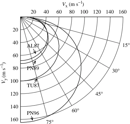
Fig. 14 shows the predictions of four models for equilibrium diving by falcons with a mass of 1 kg at an air density of 1.23 kg m−3_{. The models yield markedly different results, even}

though they share a common origin in a model introduced by Pennycuick (1971a, 1975) that partitions total drag into induced drag and other drag. The following text and Table 3 summarize the models and explain why they yield different results.

Alerstam’s model (1987) is similar to Pennycuick’s original model with the addition of allowing lift to vary with θ. The wings have maximum span at all glide angles, and the value for CD,praccounts for the drag of both the wings and the body.

Since this value is high compared with other measurements of

CD,prand CD,par, and the area of the wings is always maximum,

the values for VEare probably lower than those that real falcons

could achieve.

Tucker’s model (1987) is the one used in the present study for equilibrium diving by an ideal falcon, and it has the most variables: wing span, lift and CD,pr vary with θ. Profile and

parasite drag are separate quantities, and the moderate value for CD,par comes from measurements on a model peregrine

falcon body (Tucker, 1990). VE values are conservative, as

Table 2. Altitude loss during pull out by a 1 kg ideal falcon

from dives at various angles and speeds

θ0 VE ∆y r

(degrees) (m s−1_{) (m) (m) b}

1/bmax L1/L0 L1/W

15 43 0.9 27.8 0.27 4.6 7.8

30 67 5.5 41.1 0.20 7.1 12.1

45 83 14.7 50.1 0.17 8.8 15.0

90 101 60.2 60.2 0.16 10.8 18.3

90 155 90.6 90.6 0.13 16.5 28.0

θ0, dive angle; VE, speed; ∆y, altitude loss during pull out; r, radius

of the pull out path, b1, wing span for maximum lift during the pull

out; bmax, maximum wing span; L0, the maximum lift with maximum

wing span, is 1.7W, where W is body weight; and L1, the maximum

lift during pull out.

The VE values in the first four rows are for a parasite drag

CD,parprobably decreases as speed increases, as mentioned in

the section on Drag.

Pennycuick’s (1989) model allows wing span, but not lift or

CD,pr, to vary with θ. Constant lift causes the induced drag to

be too large at high values of θ, but the main reason for the low VEvalues is a high value for CD,parcompared with other

measurements of this quantity (Tucker, 1990). The values for

VE are somewhat higher than those for Alerstam’s (1987)

model because wing span decreases as speed increases. Pennycuick et al. (1996) suggest that CD,par should be

reduced to one-sixth of the value used in his 1989 model. The 1996 model in Fig. 14 is the 1989 model with this change, which greatly increases VE. VEvalues for all of the models are

quite sensitive to CD,par, since most of the drag at VEfor diving

falcons is parasite drag (Fig. 13).

These models suggest that real falcons in a dive could reach speeds of 100 m s−1_{and perhaps more than 150 m s}−1_{. Whether}

real falcons allow themselves to reach such speeds, and whether they tolerate the large accelerations during diving and pull out that ideal falcons do, will have to be determined by future measurements.

List of symbols b wing span

b0 wing span for minimum drag b1 wing span for maximum lift bmax maximum wing span bmin minimum wing span C a coefficient

CD,par parasite drag coefficient CD,pr profile drag coefficient CL lift coefficient

c length of mean chord line

D total drag

Di induced drag Dmin minimum drag Dmax maximum drag Dpar parasite drag Dpr profile drag

d reference length for (Re)

F magnitude of aerodynamic force

f a mathematical function

g magnitude of acceleration due to gravity

K a constant

L lift

LT lift for maximum torque L0 maximum lift at maximum span L1 maximum lift

m body mass P position vector

Q a quantity

q dynamic pressure

Re Reynolds number

r radius of an arc

t time

Sb maximum cross-sectional area of the body Sw projected area of wings

Sw,max maximum Sw Sw,min minimum Sw s distance V velocity vector

V speed through the air

VE equilibrium speed at maximum performance Ve equilibrium speed

Vmax maximum speed in a vertical dive Vx,Vy components of velocity through the air W magnitude of body weight

x, y spatial coordinates ∆y altitude drop

θ inclination of the glide path Table 3. Values of selected variables, and the maximum

speed reached in a vertical dive, for four mathematical models of diving

L Vmax

b/bmax (N) CD,pr CD,par(m s−1)

Alerstam (1987) 1 Wsinθ 0.023 − 68

Tucker (1987) 0.10−1 Wsinθ 0.036−0.012 0.18 101

Pennycuick (1989) 0.13−1 W 0.014 0.30 73

Pennycuick et al. (1996) 0.05−1 W 0.014 0.05 164

b, wing span during dive; bmax, maximum wing span; L, lift; CD,pr,

profile drag coefficient; CD,par, parasite drag coefficient; Vmax,

maximum speed in a vertical dive; W, body weight; θ, dive angle.

V_x (m s−1)

20 40 60 80 100 120 140 160

Vy

(m s

−

1 )

20

40

60

80

100

120

140

160

AL87

PN89

TU87

PN96

15°

30°

45°

60°

75°

Fig. 14. Maximum performance curves and minimum performance lines in a velocity polar diagram for a diving 1 kg falcon calculated using four different models (AL87, Alerstam, 1987; TU87, Tucker, 1987; PN89, Pennycuick, 1989; PN96, Pennycuick et al. 1996). See

text for descriptions of the models. Vx, Vy, horizontal and vertical

θ0 θat the start of pull out

µ viscosity of air

π ratio of circumference to diameter of a circle ρ density of air

ϕ angle of aerodynamic force

References

ALERSTAM, T. (1987). Radar observations of the stoops of the peregrine falcon Falco peregrinus and the goshawk Accipiter gentilis. Ibis 129, 267–273.

BROWN, L. A. (1976). British Birds of Prey. London: Collins.

CADE, T. (1982). The Falcons of the World. Ithaca: Cornell University

Press.

CLARK, W. S. (1995). How fast is the fastest bird? WildBird 9, 42–43.

CRYSTAL, D. (1997). Cambridge Factfinder. Cambridge: Cambridge University Press.

DEMENT’EV, G. P. (1951). Order Falconiformes (Accipitres). Diurnal raptors. In Birds of the Soviet Union, vol. 1 (ed. G. P. Dement’ev and N. A. Gladkov), pp. 71–379. Jerusalem: Israel Program for Scientific Translation, 1966.

HANTGE, T. (1968). Zum Beuteerwerb unserer Wanderfalken (Falco peregrinus). Orn. Mitt. 20, 211–217.

LAWSON, R. (1930). The stoop of a hawk. Essex Co. Orn. Club. pp. 79–80.

LIMPERT, R. (1992). Brake Design and Safety. Warrendale: Society of Automotive Engineering.

MARDEN, J. H. (1987). Maximum lift production during takeoff in flying animals. J. exp. Biol. 130, 235–258.

MARDEN, J. H. (1990). Maximum load-lifting and induced power output of Harris’ hawks are general functions of flight muscle mass. J. exp. Biol. 149, 511–514.

MEBS, T. (1975). Falcons and their relatives, In Grzimek’s Animal Life

Encyclopedia, vol. 7 (ed. B. Grzimek), pp. 411–431. New York: Von Nostrand Reinhold Co.

MILLER, W. H. (1979). Ocular optical filtering. In Handbook of Sensory Physiology, Vision in Invertebrates, vol. VII/6A (ed. H. Autrum), pp. 69–143. New York: Springer.

ORTON, D. A. (1975). The speed of a peregrine’s dive. The Field,

September, 588–590.

PENNYCUICK, C. J. (1971a). Gliding flight of the white-backed vulture Gyps africanus. J. exp. Biol. 55, 13–38.

PENNYCUICK, C. J. (1971b). Control of gliding angle in Rüppell’s griffin vulture Gyps rüppellii. J. exp. Biol. 55, 39–46.

PENNYCUICK, C. J. (1975). Mechanics of flight. In Avian Biology, vol. V (ed. D. S. Farner and J. R. King), pp. 1–75. New York: Academic Press.

PENNYCUICK, C. J. (1989). Bird Flight Performance. New York: Oxford University Press.

PENNYCUICK, C. J., FULLER, M. R. AND MCALLISTER, L. (1989). Climbing performance of Harris’ hawks (Parabuteo unicinctus) with added load: implications for muscle mechanics and for radiotracking. J. exp. Biol. 142, 17–29.

PENNYCUICK, C. J., KLAASSEN, M., ANDERS, K. ANDLINDSTRÖM, A. (1996). Wing beat frequency and the body drag anomaly: wind-tunnel observations on a thrush nightingale (Luscinia luscinia) and a teal (Anas crecca). J. exp. Biol. 199, 2757–2765.

PRANDTL, L. ANDTIETJENS, O. G. (1957). Applied Hydro- and Aero-mechanics. New York: Dover Publications.

REYMOND, L. (1987). Spatial visual acuity of the falcon, Falco berigora: a behavioral, optical and anatomical investigation. Vision Res. 27, 1859–1874.

SAVAGE, C. (1992). Peregrine Falcons. San Francisco: Sierra Club. THOMAS, A. L. R. (1996). The flight of birds that have wings and a

tail: variable geometry expands the envelope of flight performance. J. theor. Biol. 183, 237–245.

TUCKER, V. A. (1987). Gliding birds: the effect of variable wing span. J. exp. Biol. 133, 33–58.

TUCKER, V. A. (1988). Gliding birds: descending flight of the white-backed vulture, Gyps africanus. J. exp. Biol. 140, 325–344. TUCKER, V. A. (1990). Body drag, feather drag and interference drag

of the mounting strut in a peregrine falcon, Falco peregrinus. J. exp. Biol. 149, 449–468.

TUCKER, V. A. (1992). Pitching equilibrium wing span and tail span in a gliding Harris’ hawk, Parabuteo unicinctus. J. exp. Biol. 165, 21–41.

TUCKER, V. A. ANDHEINE, C. (1990). Aerodynamics of gliding flight in a Harris’ hawk, Parabuteo unicinctus. J. exp. Biol. 149, 469–489. TUCKER, V. A. ANDPARROTT, G. C. (1970). Aerodynamics of gliding

flight in a falcon and other birds. J. exp. Biol. 52, 345–367.

VON MISES, R. (1959). Theory of Flight. New York: Dover