Properties Relevant for Inferring Provenance

Properties Relevant for Inferring

Provenance

Author:

Abdul Ghani

Rajput

Supervisors:

Dr. Andreas

Wombacher

Rezwan Huq, M.Sc

Master Thesis

University of Twente

the Netherlands

Properties Relevant for Inferring

Provenance

A thesis submitted to the faculty of Electrical Engineering, Mathematics and Computer Science, University of Twente, the Netherlands in partial fulfillment

of the requirements for the degree of

Master of Sciences in Computer Science

with specialization in

Information System Engineering

Department of Computer Science,

University of Twente

the Netherlands

Contents

Abstract v

Acknowledgment vii

List of Figures ix

1 Introduction 1

1.1 Motivating Scenarios . . . 2

1.1.1 Supervisory Control and Data Acquisition . . . 2

1.1.2 SwissEX RECORD . . . 3

1.2 Workflow Description . . . 3

1.3 Objectives of Thesis . . . 4

1.4 Research Questions . . . 5

1.5 Thesis Outline . . . 6

2 Related work 7 2.1 Existing Stream Processing Systems . . . 7

2.2 Data Provenance . . . 8

2.3 Existing Data Provenance Techniques . . . 8

2.4 Provenance in Stream Data Processing . . . 9

3 Formal Stream Processing Model 13 3.1 Syntactic Entities of Formal Model . . . 14

3.2 Discrete Time Signal . . . 14

3.3 General Definitions . . . 18

3.4 Simple Stream Processing . . . 22

3.5 Representation of Multiple Output Streams . . . 22

3.6 Representation of Multiple Input Streams . . . 24

3.7 Formalization . . . 24

3.8 Continuity . . . 25

4 Transformation Properties 29 4.1 Classification of Operations . . . 29

4.3 Input Sources . . . 31

4.4 Contributing Sources . . . 32

4.5 Input Tuple Mapping . . . 32

4.6 Output Tuple Mapping . . . 33

5 Case Studies 35 5.1 Case 1: Project Operation . . . 35

5.1.1 Transformation . . . 35

5.1.2 Properties . . . 38

5.2 Case 2: Average Operation . . . 40

5.2.1 Transformation . . . 40

5.2.2 Properties . . . 42

5.3 Case 3: Interpolation . . . 43

5.3.1 Transformation . . . 43

5.3.2 Properties . . . 46

5.4 Case 4: Cartesian Product . . . 47

5.4.1 Transformation . . . 47

5.4.2 Properties . . . 50

5.5 Provenance Example . . . 51

6 Conclusion 55 6.1 Answers to Research Questions . . . 55

6.2 Contributions . . . 57

6.3 Future Work . . . 57

Abstract

Acknowledgment

Over the last two years, I have received a lot of help and support by many people whom I would like to thank here.

I would not have been able to successfully complete this thesis without the support of supervisors during past seven months. My sincere thanks to Dr. Andreas Wombacher, Dr. Brahmananda Sapkota and Rezwan Huq. They have been a source of inspiration for me throughout the process of the research and writing. Their feedback and insights were always valuable, and never went unused.

I owe my deep gratitude to all of my teachers, who have taught me at Twente. Their wonderful teaching methods enhanced my knowledge of the respective subject and enabled me to complete my studies in time. I also like to extend my sincere thanks to the staff of international office. Special thanks go to Jan Schut because without his support it is not possible for me to come here and complete my studies.

My roommates at the third floor at Zilverling provided a great working environ-ment. I thank them for the laughs and talks we had. I would like to thank the following colleagues and friends whose help in the study period has contributed to achieve this dream. Thanks to Fiazan Ahmed, Fiaza Ahemd, Irfan Ali, Irfan Zafar, M.Aamir, Martin, Klifman, T.Tamoor and Mudassir.

Of course, this acknowledgment would not complete without thanking my mother, brother and sister. Having supported me throughout my university study, I can-not express my gratitude enough. I hope this achievement will cheer them up during these stressful times.

My family (Nida, Fatin and Abdullah) more than deserves to be named here too. Throughout the process of my studies and my graduation research, they have been loving and supportive.

ABDUL GHANI RAJPUT

List of Figures

1.1 Workflow model based on RECORD project scenario . . . 4

2.1 Taxonomy of Provenance . . . 10

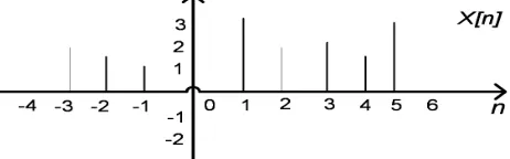
3.1 Logical components of the formal model and the idea of figure is taken from [18] . . . 15

3.2 The generic Transformation function . . . 16

3.3 Unit impulse sequence . . . 17

3.4 Unit step Sequence . . . 17

3.5 Example of a Sequence . . . 18

3.6 Sensor Signal Produces an Input Sequence . . . 19

3.7 Input Sequence . . . 20

3.8 Window Sequence . . . 21

3.9 Simple stream processing . . . 22

3.10 Multiple outputs based on the same window sequence . . . 23

3.11 Example of increasing chain of sequences . . . 26

4.1 Types of Transfer Function . . . 34

5.1 Transformation Process of Project Operation . . . 36

5.2 Input Sequence and Window Sequence . . . 37

5.3 Several Transfer Functions is Executed in Parallel . . . 38

5.4 Average Transformation . . . 41

5.5 Interpolation Transformation . . . 44

5.6 Distance based interpolation . . . 46

5.7 Cartesian Product Transformation . . . 48

5.8 Example for overlapping windows . . . 52

Chapter 1

Introduction

Stream data processing has been a hot topic in the database community in this decade. The research on stream data processing has resulted in several publications, formal systems and commercial products.

In this digital era, there are many real-time applications of stream data process-ing such as location based services (LBSs identify a location of a person) based on user’s continuously changing location, e-health care monitoring systems for monitoring patient medical conditions and many more. Most of the real-time applications collect data from source. The source (sensor) produces data con-tinuously. The real-time applications also connect with multiple sources that are spread over wide geographic locations (also called data collection points). The examples of sources are scientific data, sensor data, wireless and sensor networks. These sources are called data streams [11].

A data stream is an infinite sequence of tuples with the timestamps. A tuple is an ordered list of elements in the sequence and the timestamp is used to define the total order over the tuples. Real-time applications are specialized forms of stream data processing. In real-time applications, a large amount of sensor data is processed and transformed in various steps.

In real-time applications, reproducibility is a key requirement and reproducibil-ity means the abilreproducibil-ity to reproduce the data items. In order to reproduce the data items, data provenance is important. Data provenance [23] documents the origin of data by explicating the relationship among the input data, the algorithm and the processed data. It can be used to identify data because it provides the key facts about the origin of the data.

CHAPTER 1. INTRODUCTION

an input streamX at timenand produces output streamY. We can re-execute the same transformation processT at any later point in timen0 (withn0 > n)

on the same input streamX and generate exactly the same output streamY [1]. The ability to reproduce the transformation process for a particular data item in a stream requires transformation properties. The transformation has a number of properties for instance constant mapping. For example, if a user wants to trace back the problem to the corresponding data stream then he needs to have a constant rate of output tuple otherwise user can not handle that. Therefore one important property for inferring provenance is constant mapping or fixed mapping and we have more properties which are discussed in Chapter 4. These transformation properties are used to infer data provenance.

To this end, this thesis will present a formal stream processing model based on discrete time signal processing theory. The formal stream processing model is used to investigate different data transformations and transformation properties relevant for inferring data provenance to ensure reproducibility of data items in real-time applications.

This chapter is organized as follows. In Section 1.1, two motivating scenarios are presented. In Section 1.2, we give a detailed description of a workflow model which is based on a motivating scenario Section 1.1.2. In Section 1.3, we present the objectives of the thesis. In Section 1.4, we state our research questions and sub research questions followed by Section 1.5 that states the complete thesis outline.

1.1

Motivating Scenarios

Due to the growth in technology, the use of real-time application is increasing day-by-day in many domains such as environmental research and medical re-search. In most of these domains, the real-time applications are designed to collect and process the real-time data which is produced by sensor. In these ap-plications, provenance information is required. In order to show the importance of data provenance in stream data processing we will present two motivating scenarios in the following subsections.

1.1.1

Supervisory Control and Data Acquisition

CHAPTER 1. INTRODUCTION

points and over 3,000 public/ private electric utilities. In that system, failure of any single data collection point can disrupt the entire process flow and cause financial losses to all the customers that receive electricity from the source, due to a blackout [4].

When a blackout event occurs, the actual measured sensor data can be com-pared with the observed source data. In case of a discrepancy, the SCADA system analysts need to understand what caused the discrepancy and have to understand the data processed on the basis of the streamed sensor data. Thus, analysts must have a mechanism to reproduce the same processing result from past sensor data so that they can find the cause of the discrepancy.

1.1.2

SwissEX RECORD

Another data stream based application is the RECORD project [28]. It is a project of the Swiss Experiment (SwissEx) platform [6]. The SwissEX platform provides a large scale sensor network for environmental research in Switzerland. One of the objectives of the RECORD project is to identify how river restoration affects water quality, both in the river itself and in the groundwater.

In order to collect the environmental changes data due to river restoration, SwissEX deployed several sensors at the weather station. One of them is the sensorscope Meteo station [6]. At the weather station, the deployed sensors measure water temperature, air temperature, wind speed and some other factors related to the experiment like electric conductivity of water [28]. These sensors are deployed in a distributed environment and send the data as streaming data to the data transformation element through a wireless sensor network.

At the research centre, the researchers can collect and use the sensor data to produce graphs and tables for various purposes. For instance, a data transfor-mation element may produce several graphs and tables of an experiment. If researchers want to publish these graphs and tables in scientific journals than the reproducibility of these graphs and tables from original data is required to be able to validate the result afterwards. Therefore, one of the main requirements of the RECORD project is the reproducibility of results.

1.2

Workflow Description

CHAPTER 1. INTRODUCTION

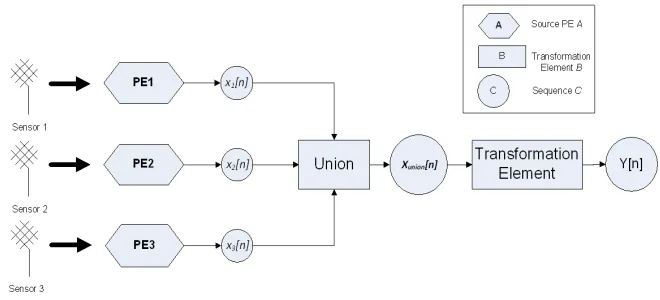
Figure 1.1: Workflow model based on RECORD project scenario

In Figure 1.1, three sensors are collecting the real-time data. These sensors are deployed in three different geographic location of a known region of the river and the region is divided into 3× 3 cells of a grid. These sensors send readings of electric conductivity of water to a data transformation element. In order to convert the sensor data in a streaming processing system, we propose a wrapper called source processing element. Each sensor is associated with a processing element namedP E1, P E2 and P E3 which provides the data tuples

in a sequence x1[n], x2[n] and x3[n] respectively. A sequence is an infinite set

of tuples/data with timestamps. These sequences are combined together (by a union operation) which generates a sequence xunion[n] as output. It contains

all data tuples sent from all the three sensors. The sequencexunion[n] will work

as input to the transformation element. The transformation element processes the tuples of the input sequence and produces an output sequence or multiple output sequencesy[n], depending on the transformation operations used. Let us look at a concrete example, at the transformation element (as shown in Figure 1.1), an average operation is configured. The average operation ac-quires tuple from xunion[n] and computing last 10 tuples/time space of the

input sequence and it executed every 5 seconds. The tuples/time space which is configured for the average operation is called a window and how often aver-age operation is executed, we call a trigger. The details of the trigger and the window are discussed in Chapter 3.

For the rest of the thesis, the example workflow model is used to define the transformation of any operation and answer the potential research questions.

1.3

Objectives of Thesis

CHAPTER 1. INTRODUCTION

• Define a formal stream processing model to do calculations over stream processing which is based on an existing stream processing model [9].

• Investigate the data transformations of SQL operations such as Project, Average, Interpolation and Cartesian product using the formal stream processing model.

• Define the formal definitions of data transformation properties.

• Prove the continuity property of the formal stream processing model.

F(∪χ) =∪F(χ)

1.4

Research Questions

In order to achieve the objectives of the thesis, the following main research questions are addressed.

• What are the formal definitions of the basic elements of a stream process-ing model that can be applied to any stream processprocess-ing systems?

• What are the suitable definitions of transformation properties for inferring provenance?

In order to answers the main research questions, the following sub questions have been defined.

• What is the mathematical formulation of a simple stream processing model?

• What are the mathematical definitions of Project, Average, Interpolation and Cartesian product transformations?

• What are the suitable properties of the data transformations?

• What are the formulas of the data transformation properties?

The formal stream processing model is a mathematical model and an important property of this mathematical model is the continuity property. It is used to provide a constructive procedure for finding the one unique behavior of the transformation. Therefore, we have another research question which is:

• How to prove the continuity property for formal stream processing model?

CHAPTER 1. INTRODUCTION

1.5

Thesis Outline

The thesis is organized as follows

• Chapter 2 gives a short review of existing stream data processing systems. It will describe what provenance metadata is, why it is essential in stream data processing and how this can be recorded and retrieved. Chapter 2 also provides the review of provenance in streaming processing.

• To derive the transfer functions of the operations, we need an existing simple stream processing model. In Chapter 3, we presented a short in-troduction to discrete time signal processing for the formalization of the formal stream processing model. Based on discrete time signal, we provide the definitions of basic elements of the formal stream processing model and discrete time representation of the stream processing.

• Chapter 4 provides the details of transformation properties and formal definitions of properties relevant for tracing provenance.

• In Chapter 5, four case studies are described where the formal stream processing model has been used and tested. At the end of the chapter, two examples are given for the case of overlapping and non-overlapping windows.

Chapter 2

Related work

This chapter introduces preliminary concepts which is used throughout this thesis. Section 2.1 starts with a brief discussion on existing stream processing systems. This includes discussions on how stream processing systems handle and process continuous data streams. Section 2.2 introduces the concept of data provenance and the importance of data provenance in stream processing systems. Section 2.3 introduces existing data provenance techniques. This chap-ter is concluded in Section 2.4, which discusses the data provenance in stream processing system.

2.1

Existing Stream Processing Systems

Stream data processing systems are more and more supporting the execution of continuous tasks. These tasks can be defined as database queries [12]. In [12] data stream processing system is defined as follows:

Data stream processing systems take continuous streams of input data, process that data in certain ways, and produce ongoing results.

Stream data processing systems are used in decision making, process control and real-time applications. Several stream data processing systems have been developed in the research as well as in the commercial sector. Some of which are described below.

STREAM [16] is a stream data processing system. The main objective of the STREAM project was memory management and computing approximate query results. It is an all purpose stream processing system but this system can not support reproducibility of query results.

CHAPTER 2. RELATED WORK

to design for adaptive query processing and shared query evaluation of sensor data. CACQ is an improved form of the Telegraph project and it has the ability to execute multiple queries concurrently [14].

Another popular system in the field of stream data processing is the Aurora sys-tem. Aurora system allows users to create the query plans by visually arranging query operators using boxes (corresponding to query operators) and links (cor-responding to data flow) paradigm [18]. The extended version of Aurora system is the Borealis [21] system. It supports distributed functionality as well.

IBM delivers a System S [19] solution for the commercial sector. The System S is a stream data processing system (it is also called stream computing system). The System S is designed specifically to handle and process massive amounts of incoming data streams. It supports structured as well as unstructured data stream processing. It can be scaled form one to thousands of computer nodes. For instance, System S can analyze hundreds or thousands of simultaneous data streams (such as stock prices, retail sales, weather reports) and deliver nearly instantaneous analysis to users who need to make split-second decisions [20].

The System S does not support the data provenance functionality and in this system data provenance is important, because later on users may want to track how data are derived as they flow through the system.

All of the above approaches do not provide the functionality of data provenance and cannot regenerate the results. Therefore, a provenance subsystem is needed to collect and store metadata, in order to support reproducibility of results.

2.2

Data Provenance

Provenance means, where is the particular tuple/data item coming from or the origin of data item or the source of a data item. In [7] provenance also defined as the history of ownership of a valued object or work of art or literature. It was originated in the field of Art and it is also called metadata. Provenance can also help to determine the quality of a data item or the authenticity of a data item [13]. In stream data processing , data provenance is important because it not only ensures the integrity of a data item but also identifies the source or origin of a data tuple. In decision support applications, data provenance can be used to validate the decision made by application.

2.3

Existing Data Provenance Techniques

CHAPTER 2. RELATED WORK

items is used to produce a set of output data items. To reproduce the output data set, one needs the query as well as the input data items. The set of input data items are referred to as Why-provenance. Where-provenance refers to the location(s) in the source database from which the data was extracted [27]. In [27], authors did not address how to deal with streaming data and associated overlapping windows. It only shows case studies for traditional data.

In [29], authors proposed a method for recording and reasoning over data prove-nance in web and grid services. The proposed method captures all information on workflow, activities and all datasets to provide provenance data. They cre-ated a service oriented architecture (SOA), where they use a specific web service for the recording and querying of provenance data. The method is only works for coarse grained data provenance (the coarse grained data provenance can be defined on relation-level) ; therefore this method cannot achieve reproducibility of results.

In [30], authors recognized a specific class of workflow called data driven work-flows. In data driven workflows, data items are first class input parameters to processes that consume and transform the input to generate derived output data. They proposed a framework called Karma2 that records the provenance information on processes as well as on data items. While their proposed frame-work is closer to the stream processing system than the majority of the research papers on workflows, it does not address the problem, specifically related to stream data processing.

To design a standard provenance model, a series of workshops and conferences have been arranged. During these workshops and conferences participants have discussed a standard provenance model, which is called the Open Provenance Model (OPM)[31]. The OPM is a model for provenance which allows provenance information to be exchanged between systems, by means of a compatibility layer based on a shared provenance model [1]. The OPM define a notion of graphs. The provenance graph is used to identify the casual relationship between artifacts, processes and agents. A limitation of the OPM is that it primarily focuses on the workflow aspect. It is not possible to define what exactly a process does. It also has an advantage that it might to be working with interoperability of different systems [31].

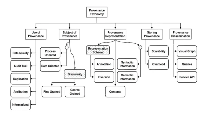
In [32] authors did a survey on data provenance techniques that were used in different projects. On the bases of their survey, they provide a taxonomy of provenance as shown in Figure 2.11_.

2.4

Provenance in Stream Data Processing

In this era, lots of real-time applications have been developed. Most of the ap-plications are based on mobile networks or sensors networks. Sensor networks,

CHAPTER 2. RELATED WORK

Figure 2.1: Taxonomy of Provenance

which are a typical example of stream data processing and commonly used in di-verse applications, such as applications which monitor the water like RECORD project, temperature and earthquake [13].

In these real-time applications, data provenance is crucial because it helps to ensure reproducibility of results and also determining the authenticity as well as quality of data items [13]. Provenance information can be used to recover the input data from the output data item. As described earlier, reproducibility is the key requirement of streaming applications and it is only possible if we can document the provenance information such as where particular data item came from, how it was generated.

First research on data provenance in stream data processing was done by IBM T.J. Watson’s Century [13]. In [15], a framework is provided (referred to as Century) with the purpose of real time analysis of sensor based medical data with data provenance support is provided. In the architecture of Century, a subsystem called data provenance is attached. This subsystem allows users to authenticate and track the origin of events processed or generated by the sys-tem. To achieve this, authors designed a Time Value Centric (TVC) provenance model, which uses both process provenance (defined at workflow level) and data provenance (derivation history of the data) in order to define the data item and input source which contributed to a particular data item. However, the approach has only been applied in the medical domain. This paper did not mention formal description of properties (discussed in Chapter 4) relevant for inferring provenance.

CHAPTER 2. RELATED WORK

provenance collection in sensor based environmental data stream. In this paper, authors focus on identifying properties that represent provenance of data item from real time environmental data streams. The three main challenges described in [34] are given below:

• Identifying the small unit (data item), for which provenance information is collected.

• Capturing the provenance history of streams and transformation states.

• Tracing the input source of a data stream after the transformation is completed.

A low overhead provenance collection model has been proposed for a meteorol-ogy forecasting application.

In [5], authors report their initial idea of achieving fine-grained data provenance using a temporal data model. They theoretically explain the application of the temporal data model to achieve the database state at a given point in time.

Recently [1], proposed an algorithm for inferring fine grained provenance in-formation by applying a temporal data model and using coarse grained data provenance. The algorithm is based on four steps; first step is to identify the coarse grained data provenance (it contains information about the transforma-tion process performed by that particular processing element). Second step is to retrieve the database state. Third step is to reconstruct the processing window based on information provided by the first two steps. The final step is to infer the fine grained data provenance information. In order to infer fine grained data provenance, authors have provided the classification of transformation proper-ties of processing elements, i.e., operations only for constant mapping opera-tions. Such properties are the input sources, contributing sources, input tuple mapping and output tuple mapping. Authors have implemented the algorithm into a real time stream processing system and validated their algorithm.

Chapter 3

Formal Stream Processing

Model

The goal of this chapter is to provide a mathematical framework for stream data processing which is based on discrete time signal processing theory. It can be named as formal stream processing model.

The discrete time signal processing is the theory of representation, transforma-tion and manipulatransforma-tion of signals and the informatransforma-tion they contain [22]. The discrete time signal can be represented as a sequence of numbers. The discrete time transformation is a process that maps an input sequence into an output sequence. There are a number of reasons to choose discrete time signal pro-cessing to formalize the stream data propro-cessing. One important reason is that, the discrete time signal processing allows for the system to be event-triggered, which is often the case in stream data processing. Another reason is that, one of the objectives of the stream data processing is to perform real-time processing on real-time data. Therefore, the discrete time signal processing is common to process real-time data in communication systems, radar, video encoding and stream data processing [22].

CHAPTER 3. FORMAL STREAM PROCESSING MODEL

stream processing model is given.

3.1

Syntactic Entities of Formal Model

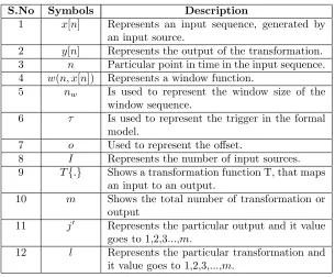
The symbols, formulas and interpretation used in formal stream processing model are syntactic entities [24]. The syntactic entities are the basic require-ments to design a formal model [24]. Figure 3.1 shows that the formal stream processing model is based on symbols, string of symbols, well-formed formulas, interpretation of the formulas and theorems. In order to define a trasformation element, syntactic entities of the formal stream processing model are required because syntactic entities are used to define the transformation element.

The list of symbols, used in our formal stream processing model, and their description [25] are given in Table 3.1.

S.No Symbols Description

1 x[n] Represents an input sequence, generated by an input source.

2 y[n] Represents the output of the transformation. 3 n Particular point in time in the input sequence. 4 w(n, x[n]) Represents a window function.

5 nw Is used to represent the window size of the

window sequence.

6 τ Is used to represent the trigger in the formal model.

7 o Used to represent the offset.

8 I Represents the number of input sources. 9 T{.} Shows a transformation function T, that maps

an input to an output.

10 m Shows the total number of transformation or output

11 j0 Represents the particular output and it value goes to 1,2,3...,m.

12 l Represents the particular transformation and it value goes to 1,2,3,...,m.

Table 3.1: List of Symbols used in FSPM

3.2

Discrete Time Signal

CHAPTER 3. FORMAL STREAM PROCESSING MODEL

CHAPTER 3. FORMAL STREAM PROCESSING MODEL

and the transformation of these signals [22]. The mathematical representation of the discrete time signal is defined below:

Discrete time signal:n∈Z→x[n]

Where

indexnrepresents the sequential values of time,

x[n], thenthnumber in the sequence, is called a sample. the complete sequence is represented as{x[n]}.

In the used stream processing model, a stream is called a sequence. The formal model is process stream or set of streams. Therefore we can say that, a stream is simply a discrete time sequence or discrete time signal.

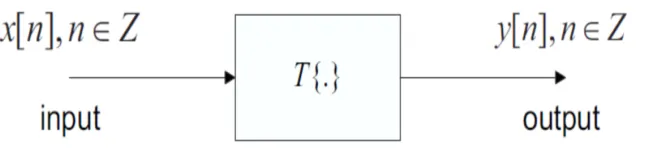
A transformation is a discrete time system. A discrete time system maps an in-put sequence{x[n]}to an output sequence{y[n]}; An equivalent block diagram is shown in Figure 3.2.

Figure 3.2: The generic Transformation function

In order to define a transformation of an operation, some basic sequences and sequence of operations are required.

Unit Impulse

The unit impulse or unit sample sequence (Figure 3.3) is a generalized function depending onnsuch that it is zero for all values of n except when the value of

nis zero.

δ[n] =

1 n= 0

CHAPTER 3. FORMAL STREAM PROCESSING MODEL

Figure 3.3: Unit impulse sequence

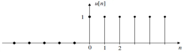
Unit Step

The unit step response or unit step sequence (Figure 3.5) is given by

u[n] =

1 n≥0

0 n≤0

The unit step response is simply an on-off switch which is very useful in discrete time signal processing.

Figure 3.4: Unit step Sequence

Delay or shift by integer k

y[n] =x[n−k] -∞< n <∞

when,k≥0, sequence ofx[n] shifted bykunits to the right.

k <0,sequence ofx[n] shifted byk units to the left.

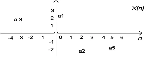
Any sequence can be represented as a sum of scaled, delayed impulses. For example the sequencex[n] in Figure 3.5 can be expressed as:

CHAPTER 3. FORMAL STREAM PROCESSING MODEL

Figure 3.5: Example of a Sequence

More generally, any sequence can be represented as:

y[n] =

∞

X

k=−∞

x[k]δ[n−k]

Finally, these concepts of discrete time signal theory help us to represent the formal definitions of stream processing model. The formal model will allow us to define the properties relevant for inferring provenance.

3.3

General Definitions

The fundamental elements of any stream processing system are data streams, transformation element, window, trigger and offset. There are number of defini-tions available in the literature for these fundamental elements. In this thesis we try to provide the formal definition of these elements. The element definitions are as follows.

Input Sequence

In our model, the input data arrives from one or more continuous data streams. Normally, these data streams are produced by sensors. These data streams are represented as input sequences in our model. The input sequence represents the measurement/record of a sensor. The input sequence contains more than one element. Each of these elements is called a sample which represents one measurement [22].

Definition 1 Input Sequence: An input sequence is a data stream used by a transformation function. It is a sequence of number x, where the nth number in the input sequence is denoted asx[n]:

CHAPTER 3. FORMAL STREAM PROCESSING MODEL

Figure 3.6: Sensor Signal Produces an Input Sequence

Where n is an integer number which represents the measurement/record of a sensor.

Note that from this definition, an input sequence is defined only for integer values ofnand refers to the complete sequence simply by{x[n]}. For example, the infinite length sequence as shown in Figure 3.6 is represented by the following sequence of numbers.

x={..., x[1], x[2], x[3]...}

Transformation

The transformation is a transfer function which takes finitely many input se-quences as input and gives finitely many sese-quences as output. The number of input and output depends on an operation. The formal definition of the transformation is given as:

Definition 2 Transformation: Let{xi[n]} be the input sequences and{yj0[n]}

be the output sequences for 1≤i≤I and1 ≤j0 ≤m. A transformation is a transfer function T defined as:

m Y

j0₌₁

yj0[n] =T{

I Y

i=1

xi[n]}.

Where m is the total number of output and I is the total number of input se-quence.

Window

CHAPTER 3. FORMAL STREAM PROCESSING MODEL

window is defined to select the most recent samples of the input sequence. A window always consists of two end-points and a window size. The end-points are moving or fixed. Windows are either time based or tuple based [1]. In this thesis, we used time based window. Why we used time based window? Because we have a model that supports only time instead of tuple which is based on IDs. The formal stream processing model supports time based sliding window because a time stamp is associated with each sample of the input sequence. The sliding window is a window type in which both end-points move. In the sliding window, the window size is always constant. To represent the window in our formal model, we have defined a window function. The formal definition is given as follows:

Definition 3 Window Function: A window function is applied on the input sequence (Definition 1) in order to select a subset of the input sequence{x[n]}.

This function selects subset of nw elements in the sequence where nw is the

window size. Window function is defined as:

w(n,{x[n]}) =

nw−1

X

k=0

x[n0]δ[n−n0−k] − ∞< n0, n <∞

which is also equivalent to:

w(n,{x[n]}) =

n X

k=n−nw+1

x[n0]δ[n0−k] − ∞< n0, n <∞ (3.2)

The output of the window functionw(n,{x[n]}) is called the window sequence. The window sequence is nothing more than a sum of delayed impulses (defined in Section 3.2) multiplied by the corresponding samples of the sequence{x[n]}

at the particular point in timen. The resulting sequence can be represented in terms of time. Example 3.1, describing the working of window function.

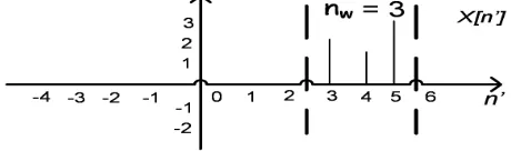
Example 3.1Suppose we have an input sequence{x[n]}as shown in the Figure 3.7. To select subset of the sequence, window function is applied on the input sequence.

CHAPTER 3. FORMAL STREAM PROCESSING MODEL

The samples involved in computation of the window sequence arek = 3 to 5 with window sizenw= 3 andn= 5. The result of the window function is shown

in Figure 3.8. By putting these parameters to the window function formula, we get:

Figure 3.8: Window Sequence

w(5,{x[n]}) =

5

X

k=5−3+1

x[n0]δ[n0−k]

w(5,{x[n]}) =

5

X

k=3

x[n0]δ[n0−3]

w(5,{x[n]}) =x[n0]δ[n0−3] +x[n0]δ[n0−4] +x[n0]δ[n0−5] whenn0 is 3 from replicated sequence therefore, we get:

w(5,{x[n]}) =x[3]

Similarly the output of thew(5,{x[n]}) =x[4],when n0_{= 4 andw(5,{x[n]}) =}

x[5],whenn0_{= 5.}

Trigger Rate

A trigger rate represents the data driven control flow of the data workflow. Data-driven workflows are executed in an order determined by conditional expressions [8]. Triggers are important in a stream processing. It is used to specify when a transformation element should execute. In general, there are two types of triggers, namely time based triggers and tuple based triggers. A time based trigger executes at fixed intervals, while a tuple based trigger executes when a new tuple arrives [1]. The formal model is based on time based triggers since the formal model is based only for time (we do not have a model for IDs).

CHAPTER 3. FORMAL STREAM PROCESSING MODEL

how many samples are skipped at the beginning of the total record before samples are transferred to the window. Which is defined as:

δ[n%τ−o]

The transformation element is defined for all values ofn,based on the trigger the transformation element is only supposed to be defined at the moments where the trigger is enabled. Thus, for a transformationT{.}, a trigger is applied with a unit sample(i.e. δ[n%τ−o] = 1).

3.4

Simple Stream Processing

The simple stream processing is based on a transformation function that maps input data contained in a window sequence producing an output sequence, where the transformation function is executed after arrival of everyτ elements of the input sequence. It shows how to process and integrate the input sequence to produce the output sample as shown in Figure 3.9.

Figure 3.9: Simple stream processing

Based on the above definition, the simple possible stream processing can be defined mathematically as,

y[n] =δ[n%τ−o]T{w(n,{x[n]})} − ∞< n <∞ (3.3) with window sizenw, trigger offsetoand trigger rateτ.

3.5

Representation of Multiple Output Streams

CHAPTER 3. FORMAL STREAM PROCESSING MODEL

y1[n] =δ[n%τ−o]T1{w(n,{x[n]})}

:

yl[n] =δ[n%τ−o]Tl{w(n,{x[n]})}

To represent the multiple outputs of the transformation element, we used the concept of the direct product. The direct product is defined on two algebras X and Y, giving a new one. It can be represented as infix notation×, or prefix notationY. The direct product of X ×Y is given by the Cartesian product of X,Y together with a properly defined formation on the product set.

Definition 5 Multiple outputs: Lety1[n], y2[n], y3[n]...ym[n]be the outputs of

T1{.}, T2{.}, T3{.}, ...Tm{.} based on the same window sequence w(n,{x[n]})

of input sequence for all values of n, then multiple output can be represented by

m Y

j0₌₁

yi[n] = m Y

l=1

Tl{.} m

Y

j0₌₁

yi[n] = m Y

l=1

δ[n%τ−o]Tl{w(n,{x[n]})}

wheremis the total number of output.

Figure 3.10 shows the graphical representation of multiple outputs based on the same window sequence. The direct product of the output sequence can be interpreted as a sequence of output tuples. In definition 5, we assumed that the number of output is fixed tom.

CHAPTER 3. FORMAL STREAM PROCESSING MODEL

3.6

Representation of Multiple Input Streams

The concept of multiple input streams is common in stream data processing and in mathematics. For instance, union and Cartesian Product can take more than one sequence as input. In order to carry out the transformation of these processing elements, we have to extend the simple stream processing model to support multiple input streams.

Definition 6 Multiple input streams: Let us we have multiple window sequences

w(n1,{x1[n]}), ....w(ni,{xi[n]}) and each window has a different window size

nw1...nwi. Let these windows are input to a transformation function such as:

y[n] =δ[n%τ−o]T{w(n1,{x1[n]}), ....w(ni,{xi[n]})} − ∞< n0, n <∞

Multiple input streams can also be defined in terms of a direct product again, that is:

y[n] =δ[n%τ−o]T{ I Y

i=1

w(ni,{xi[n]})} − ∞< n <∞

where I is the total number of input stream/source.

3.7

Formalization

This section combines the definitions introduced before in order to define the formal stream processing model. Equation 3.4 shows the mathematical descrip-tion of the formal stream processing model. This formal model will be used to do calculations over stream processing. In Equation 3.4, the structure of the input sequence and the output sequence is not considered. It is, therefore, pos-sible to include the more complex data structure ofyj0[n] andx_i[n] in Equation

3.4. The resulting formal stream processing which includes more complex data structure is given in Equation 3.5.

m Y

j0₌₁

yj0[n] =δ[n%τ−o]

m Y l=1 Tl{ I Y i=1

w(ni,{xi[n]})} − ∞< n <∞ (3.4)

m Y

j0₌₁

dj0,y_j0

Y

j00₌₁

yj0_,j00[n] =δ[n%τ−o]

m Y l=1 Tl{ I Y i=1

w(ni, d_xi Y

ji=1

{xi,ji[n]})} −∞< n <∞

CHAPTER 3. FORMAL STREAM PROCESSING MODEL

j0andl= 1,2,3...m,wherembeing the maximum number of outputs of the processing element

dj0_,y

j0 is the dimensionality of the data structure of the j

0_thoutput

sequenceyj0

I is the number of input sequences

dxi is the dimensionality of the data structure of the ith input

se-quencexi

In this thesis, dimensionality of the input data is not considered because the data structure information of the input data is not available in advance. The formal model (without considering the complex data structure) Equation 3.4 is used to identify the data transformation and transformation properties for inferring provenance, which are discussed in next chapter.

3.8

Continuity

In this section, we provide a simple proof of a continuity property of the formal stream processing model. The proof of the method is essentially the same as in [26] but the contribution here the proof of continuity property using the notations of formal stream processing model.

As per the Kahn Process Network [26], let{x[n]}denotes the sequence of values in the stream, which is itself totally ordered set. In our formal stream processing model, the order relationship is not present because every sequence is defined from−∞to∞, as shown in Figure 3.11.

To define a partial order relatioship in our formal model, let us consider a prefix ordering of sequences, wherex1[n] vx2[n], if x1[n] is a prefix of x2[n] (i.e., if

the first values ofx2[n] are exactly those in x1[n]) inX. WhereX denotes the

set of finite and infinite sequences as shown in Equation 3.6.

X={x1[n], x2[n], x3[n], ...}=

∞

[

i=1

{xi[n]} 1≤i≤ ∞ (3.6)

In Equation 3.6, X is a complete partial order set, if it holds the following relationship between sequences.

xi[n]vxj[n]⇔xi[n] =xj[n]·u[−i]

CHAPTER 3. FORMAL STREAM PROCESSING MODEL

Figure 3.11: Example of increasing chain of sequences

[26]. A least upper bound (LUB), written tX, is an upper bound that is a prefix of every other upper bound. The term (xj[n]·u[−i]) indicates that when

xj[n] is multiplied with the unit step sequence then we get thexi[n] sequence.

In our formal stream processing model, usually T is executed on a sequence. Now we can extend the definition of T in order to execute and support chain of sequences such as:

T(X) = [

x[n]X

T{x[n]}

Definition: Let X and Y be the CPO’s. A transformation T : X → Y is continuous if for each directed subset x[n] of X, we have T(tX) = tT(X). We denote the set of all continuous transformation from X to Y by [X →Y].

In our formal stream processing model, a transformation takesm input andn

outputs such asT :Xm_→Yn_{.Let a transformation is defined as below:}

T(x[n]) =

y[n], if x[n]vX

0 otherwise

Theorem: The above transformation is Continuous.

Proof. Consider a chain of sequencesX ={x1[n], x2[n], x3[n], ...},we need to

show thatT(tX) =tT(X).WriteT(X) = [

x[n]X

CHAPTER 3. FORMAL STREAM PROCESSING MODEL

Taking R.H.S:

tT(X) =t{T(x1[n]), T(x2[n]), ...}

Since X is an increasing chain, it has a least upper bound as per the partial order relationship defined above. Suppose the LUB isx[n], then output is:

tT(X) =t{T(x1[n]), T(x2[n]), ..., T(x[n])}

tT(X) =x[n] =y[n] Similarly for L.H.S:

T(tX) =T(t{x1[n], x2[n], ..., x[n]}

T(tX) =x[n] =y[n]

Chapter 4

Transformation Properties

The goal of this chapter is to provide the formal definitions of transformation properties for inferring provenance. In Section 1.2, a workflow model was de-scribed, in which transformation is an important element. The transformation has a number of properties that makes it useful for inferring provenance. These transformation properties are: input sources, contributing sources, input tuple mapping, output tuple mapping and mapping of operations. These are classified and discussed in [1] as required for reproducibility of results in e-science applica-tions. Based on this classification, the formal definitions of the transformation properties are provided in this chapter.

The remainder of the chapter is organized as follow. Section 4.1 provides the classification of operation. Section 4.2 explains the mapping of operations and provides the formal definition of mapping. Section 4.3 describes the in-put sources property and its formal definition. Section 4.4 discusses about the contributing sources property and provides the formal definition. Section 4.5 ex-plains and defines the formal definition of input tuple mapping. Finally, Section 4.6 defines the output tuple mapping and its formal definition.

4.1

Classification of Operations

To formalize the definitions of transformation properties, the data transfor-mation of four SQL operations are considered. These are: Project, Average, Interpolation and Cartesian product. Each of these data transformations have a set of properties, such as the ratio of mapping from input to output tuples is a transformation property. The explanation of all these properties is described in Table 4.1.

CHAPTER 4. TRANSFORMATION PROPERTIES

product are constant mapping operations, which are separated by black solid line. The Select operation is a variable mapping operation which is not consid-ered in this thesis.

Figure 4.1 shows that the Project, Average and Interpolation operation are single input source operations. The Cartesian product operation is a multiple input source operation.

It also shows that Project transformation takes a single element of the input sequence and produces a single element at the output sequence. Thus, the ratio is 1 : 1. The Average transformation takes three input elements of the input sequence and produced single output, therefore the ratio is 3 : 1.

CHAPTER 4. TRANSFORMATION PROPERTIES

4.2

Mapping of Operations

Based on the classification of operations described in Section 4.1, the formal definition of a mapping is defined in this section. The two types of transfor-mations are possible: constant mapping and variable mapping transfortransfor-mations. The constant mapping transformations have a fixed ratio. The variable map-ping transformations do not maintain a fixed ratio of input to output mapmap-ping as described in Table 4.1. Let us give the formal definition.

Definition 7 Constant Mapping Transfer Function: T :{w(n,{x[n]})} → {y[n]}

is called constant mapping transfer function if the mapping ratio of{w(n,{x[n]})}

to{y[n]}is fixed for all values of n. If it is not fixed, then it is a variable map-ping.

4.3

Input Sources

In our formal stream processing model, one of the important transformation properties is input sources. This property is used to find the number of input sources that contribute to produce an output tuple.

The input sources are input sequences (see Definition 1). The transfer functions takes one or more input sources, processes them and produces one or more derived output sequences. The single input source transfer functions do have a single input sequence, while multiple input source transfer functions have multiple input sequences as inputs. Let us give a formal definition.

Definition 8 Input Sources: Let y[n] be an output sequence of a transfer func-tion T, where T is applied on one or more input sequences as per Definifunc-tion 6, then:

y[n] =δ[n%τ−o]T{ I Y

i=1

CHAPTER 4. TRANSFORMATION PROPERTIES

where I is used to denote the number of input sources contributing to T to produce the output, I∈N, whereNis the natural number. Therefore:

Input sources=

M ultiple if I >1

Single else

4.4

Contributing Sources

The formal definition of this property will be used to find the creation of an output sample is based on samples from a single or multiple input sequences. This property is only applicable for those transformations which takes I > 1 input sequences as an input. The formal definition of the property is given below.

Definition 9 Contributing Sources: Let T be a transfer function which have multiple input sources as input, such as w(n1,{x1[n]})×...×w(n0i,{xi[n0]}),

then contributing sources property defined as:

T{w(n1,{x1[n]})×...×w(n0i,{xi[n0]})}=T ( I

Y

i=1

w(ni,{xi[n]}) )

Contributing sources=

          

M ultiple F or I >1 and

each I is contributed in T

Single For I>1and

only a single source is contributed in T

N ot Applicable ForI= 1

4.5

Input Tuple Mapping

The input tuple mapping property is used to find a given sample, related to the input source that is used by the transfer function. The formal definition is as follows:

Definition 10 Input Tuple Mapping (ITM): Let T be a transfer function and applied on a window (see definition 3){w(n,{x[n]})},which is equivalent to:

T{w(n,{x[n]})}=T

( n

X

k=n−nw+1

x[n0]δ[n0−k]

)

− ∞< n0, n <∞

CHAPTER 4. TRANSFORMATION PROPERTIES

4.6

Output Tuple Mapping

The most important and difficult property is the output tuple mapping for inferring provenance data. It depends on input tuple mapping as well as on an input source. In this property, dimensionality of input data is important beacuse the output data dimensionality is different from the input data dimensionality. But In this thesis, we did not consider the dimensionality of the input data. Output tuple mapping distinguishes whether the execution of a transformation produces a single or multiple output tuple per input tuple mapping [1]. The output tuple mapping is a decimal or a fractional number when it is calculated. The formal definition is given as:

Definition 11 Output Tuple Mapping (OTM): Let T be a transformation that maps thenw(windowsize) samples per source to produce the m number of output

samples, then the output tuple mapping is defined as:

OT M =r× I X

i=1

IT Mi

M ultiple OT M >1 Single otherwise

where OT M =output tuple mapping

IT Mi=input tuple mapping per source

r = m

I X

i=1

nwi

CHAPTER 4. TRANSFORMATION PROPERTIES

Chapter 5

Case Studies

The primary goal of this chapter is to derive the transformation of the Project, Average, Interpolation and Cartesian product to exemplify the formal stream processing model and formal definitions of transformation properties described in the previous chapters.

5.1

Case 1: Project Operation

5.1.1

Transformation

This section derives the transformation definition of Project operation using the formal stream processing model. We begin by explaining the concept of Project operation.

The Project operation is a SQL operation which is also called projection. A project is an unary transformation that can be applied on a single input se-quence. The transformation process takes the input sequence (see Definition 1) and computes the sub-samples of the input sequence. In other words, it reduces thenthsample from the input sequence. Similarly in the databases, projection of a relational database table is a new table containing a subset of the original columns.

Figure 5.1 shows the graphical representation of the project transformation process and also shows that the sensor produces an input sequence which is

CHAPTER 5. CASE STUDIES

transformation i.e. Y1[n],Y2[n] and Ym[n] as shown in Figure 5.1. All outputs

are associated with the same timen.

Figure 5.1: Transformation Process of Project Operation

Now using the concept of project operation which is defined above, the transfer function of project can be derived using the formalization Equation 3.4 which is:

m Y

j0₌₁

yj0[n] =δ[n%τ−o]

m Y

l=1

Tl{ I Y

i=1

w(ni,{xi[n]})} − ∞< n <∞

Put the value ofI = 1 in the above equation, because the project is an unary operation. we get:

m Y

j0₌₁

yj0[n] =δ[n%τ−o]

m Y l=1 Tl{ 1 Y i=1

w(ni,{xi[n]})} − ∞< n <∞

As we have described earlier that the total number of outputs for the project operation is equal to the window size which is m = nw, therefore the above

equation becomes:

nw

Y

j0₌₁

yj0[n] =δ[n%τ−o]

nw Y l=1 Tl ( 1 Y i=1 n X

k=n−nw+1

xil[n

0_]δ[n0_−k]

!)

−∞ ≤n0, n≤ ∞

The project transformation simply takes the input sequence{x[n]} to the right by l−nw samples to form the output where Tl denotes the total number of

CHAPTER 5. CASE STUDIES

nw

Y

j0₌₁

yj0[n] =δ[n%τ−o]

nw

Y

l=1 1

Y

i=1

xil[n−nw+l] − ∞< n <∞ (5.1)

where

xilis the input sequence, where the value ofi= 1 which means that

single input source is participating and l represents the particular point sample in time.

nw is the window size and being the maximum number of outputs

by the project operation.

ois the offset value initially we consider offset to be zero andτ is a trigger rate.

Example 5.1 Suppose an input sequence (as shown in Figure 5.2) is applied on a project transformation. The window function is applied on input sequence with nw= 3 at the point in time n= 5. The transfer function is executed after

arrival of every 3 elements in the sequence and the trigger offset is 2.

Figure 5.2: Input Sequence and Window Sequence

By putting the valuesnw= 3, I= 1, τ = 3 and o= 2 in Equation 5.1, we get:

3

Y

j0₌₁

yj0[n] =δ[n%τ−o]

3

Y

l=1

x1l[n−nw+l]

The output of the above equation is multiple as per the Definition 5. It can be modeled as transformations in parallel producing several outputs as shown in Figure 5.3.

In Figure 5.3,Tl takes the window sequence as an input sequence and it

pro-duces multiple outputs which areT1, T2 and T3. Therefore, the general output

CHAPTER 5. CASE STUDIES

Figure 5.3: Several Transfer Functions is Executed in Parallel

3

Y

j0₌₁

yj0[n] =x₁

1[n−nw+ 1]×x12[n−nw+ 2]×x13[n−nw+ 3] Let us start with the definition ofT1. It takes window sequence with the

fol-lowing parameters nw = 3, l = 1 and n = 5 and translate it in the following

steps.

y1[n] =x11[n−nw+ 1]

y1[n] =x11[5−3 + 1]

y1[n] =x11[3] =T1

The transformation function T2 executes the next sample with the following

parametersnw= 3, l= 2 andn= 5,the output becomes:

y2[n] =x12[n−nw+ 2]

y2[n] =x12[5−3 + 2]

y2[n] =x12[4] =T2

This process is performed continuously until all the transformations are exe-cuted.

5.1.2

Properties

In the previous section, the project transformation is defined to test the formal definitions of transformation properties (as we have defined in Chapter 4). We have to test the following properties:

• Input Sources

• Contributing Sources

• Input Tuple Mapping

CHAPTER 5. CASE STUDIES

Input Sources

This property checks that transfer functions take single or multiple input sources as input that contributes to produce an output sample. According to Definition 8, the value of I in our formal model is used to identify the number of input sources that contribute to produce the output. The derived project transforma-tion is:

nw

Y

j0₌₁

yj0[n] =δ[n%τ−o]

nw Y l=1 1 Y i=1

xil[n−nw+l] − ∞< n <∞

Now compare the project transformation definition with the formal stream pro-cessing model, which is

m Y

j0₌₁

yj0[n] =δ[n%τ−o]

m Y

l=1

Tl{ I Y

i=1

w(ni,{xi[n]})} − ∞< n <∞

As we can see, the value ofIin the project transformation is equal to 1, therefore the project transformation is a single input source operation.

Contributing Sources

According to Definition 9, the contributing sources property is only applica-ble for those transformations which have multiple input sources. In case of the project transformation this property is not applicable because the project transformation has a single input source as shown in Equation 5.1.

Input Tuple Mapping

According to Definition 10, the input tuple mapping of the project transfor-mation is single. The project transfortransfor-mation Equation 5.1 indicates that the output of the project transformation is a single sample i.e. xil[n−nw+l] instead

of accumulated sum of the value at indexnand all previous values of the input sequence{x[n]}.

Output Tuple Mapping

CHAPTER 5. CASE STUDIES

OT M =r× I X

i=1

IT Mi

M ultiple OT M >1 Single otherwise

where OT M =output tuple mapping

IT Mi=Input tuple mapping per source

r = m

I Y

i=1

nwi

where I is the total number of input sources

Therefore to calculate the output tuple mapping of the project transformation, the value ofmand the value of the input tuple mapping is required. The input tuple mapping has been already calculated in previous section. The input tuple mapping is one. The total number of output can easily derived from the project transformation equation:

nw

Y

j0₌₁

yj0[n] =δ[n%τ−o]

nw

Y

j0₌₁

1

Y

i=1

xil[n−nw+l] − ∞< n <∞

The above equation indicates that the total number of output produced by the project transformation ism=nw,therefore by putting the values in the output

tuple mapping formula. we get:

OT M =r× I X

i=1

IT Mi

OT M = m

1 Y i=1 nwi × 1 X i=1

IT Mi

OT M = nw

nw

×1 = 1

The result of Definition 11 is interpreted that the output tuple mapping of project transformation is 1.

5.2

Case 2: Average Operation

5.2.1

Transformation

CHAPTER 5. CASE STUDIES

a SQL aggregate operation and returns a single value, using the values in a table column [35]. Figure 5.4 shows the generic process of the average transformation. It also shows that the average is calculated by combining the values from a set of input and computing a single number as being the average of the set.

Figure 5.4: Average Transformation

From the concept of the average operation, the average transformation can be derived using the following equation:

m Y

j0₌₁

yj0[n] =δ[n%τ−o]

m Y l=1 Tl{ I Y i=1

w(ni,{xi[n]})} − ∞< n <∞

In the above equation, we can put the value ofI = 1 and the value of m= 1 since the average returns a single sample, using samples in an input sequence. So, the resulting equation is:

1

Y

j0₌₁

yj0[n] =δ[n%τ−o]

1 Y l=1 Tl{ 1 Y i=1

w(ni,{xi[n]})} − ∞< n <∞

1

Y

j0₌₁

yj0[n] =δ[n%τ−o]

1 Y l=1 Tl ( ₁ Y i=1 n X

k=n−nw+1

xil[n

0_]δ[n0_−k]

!)

− ∞ ≤n0, n≤ ∞

In mathematics, the average of n numbers is given as 1/n

n X

i=1

ai where ai are

CHAPTER 5. CASE STUDIES

1

Y

j0₌₁

yj0[n] =δ[n%τ−o]

1 Y l=1 1 Y i=1 1 nw n X

k=n−nw+1

x1[k]

!

− ∞< n <∞ (5.2)

where

x1is the input sequence andyj0[n] is the output sequence where j0

is the number of output which is equal to 1.

nw is the window size and n is the point in time at which we are

interested to start calculating the average.

o is the offset value, initially it is considered to be zero and τ is a trigger rate.

5.2.2

Properties

Input Sources

The input sources property checks whether the average transformation takes single or multiple input sources as input (as per Definition 8). The property can be checked by looking at the average transformation Equation 5.2. In Equation 5.2, the value of I = 1. Therefore, average is a single input source transformation.

Contributing Sources

Same as the project transformation, the contributing sources property is not applicable on the average transformation because Equation 5.2 indicates that the average transformation has a single input source as input.

Input Tuple Mapping

The input tuple mapping property of the average transformation is multiple since output of the average transformation is the accumulated sum of the value at indexnand all previous values of the input sequencex[n] that is:

n X

k=n−nw+1

x1[k] =x1[n−nw+ 1] +x1[n−nw+ 2] +...+x1[k]

CHAPTER 5. CASE STUDIES

k= (n−n+nw+ 1)−1

k=nw

So, the average transformation has multiple input tuple mapping i.e. nw.

Output Tuple Mapping

To calculate the output tuple mapping of the average transformation, Definition 11 is used. The formula for output tuple mapping is:

OT M =r× I X

i=1

IT Mi

OT M = m

1

Y

i=1

nwi ×

1

X

i=1

IT Mi

OT M = 1

nw

×nw= 1

The result of the OTM formula is 1 which means that the output tuple mapping of the average transformation is 1.

5.3

Case 3: Interpolation

5.3.1

Transformation

The Interpolation is an important function in many real-time applications such as the RECORD project (described in Section 1.2) and has been used for years to estimate the value at an unsampled location. It is important for visualization such as generation of contours.

There exist many different methods of interpolation. The most common ap-proaches are weighted average distance and natural neighbors. The deatials of these approaches are available in [36]. In this thesis only weighted distance based interpolation transformation is described.

CHAPTER 5. CASE STUDIES

is used to derive the transformation of interpolation operation using the formal stream processing model.

Figure 5.5 shows the generic process of the interpolation transformation. It shows that the interpolation transformation takes a number of input samples from an input sequence and produces a set of output samples. In Figure 5.5, the interpolation takes 2 input samples and produces 6 output samples. Sim-ilarly, if it takes 3 input samples then it produces 9 output samples therefore interpolation is a constant mapping operation (as we have described in Section 4.1).

Figure 5.5: Interpolation Transformation

To derive the interpolation transformation, we can use the formal model Equa-tion 3.4:

m Y

j0₌₁

yj0[n] =δ[n%τ−o]

m Y

l=1

Tl{ I Y

i=1

w(ni,{xi[n]})} − ∞< n <∞

CHAPTER 5. CASE STUDIES

m Y

j0₌₁

yj0[n] =δ[n%τ−o]

m Y l=1 Tl{ 1 Y i=1

w(ni,{xi[n]})} − ∞< n <∞ m

Y

j0₌₁

yj0[n] =δ[n%τ−o]

m Y l=1 Tl ( 1 Y i=1 n X

k=n−nw+1

xi[n0]δ[n0−k] !)

− ∞< n.n0<∞

Suppose that we have an input sequence{x[n]} and we can apply the window function on the input sequence to select a subset of the samples (of window size

nw) at the given point in time n, therefore the above equation become, m

Y

j0₌₁

yj0[n] =δ[n%τ−o]

m Y l=1 1 Y i=1 n X

k=n−nw+1

x1[k]

!

Given a set of samples to which a point P(x,y) is attached as shown in Figure 5.6. The point P is user-defined. In Figure 5.6, black circles are samples involved in the interpolation and gray circle is a new sample which is being esitmated. The weight assigned to each sample is typically based on the square of the distance from the black to gray circle. Therefore the above equation becomes:

m Y

j0₌₁

yj0[n] =δ[n%τ−o]

m Y l=1 1 Y i=1 n X

k=n−nw+1

λi,l·x1[k]

!

where

λi,l=

1/C+d2

n,l

Pn

k0=n−nw+11/C+d2n,l

λi,l the weight of each sample (with respect to the interpolation

sample i.e. gray circle) used in the interpolation process,

d2

i,l is the distance between sample n and the location being

esti-mated

C is the small constant for avoiding∞condition So, the interpolation transformation is defined as,

m Y

j0₌₁

yj0[n] =δ[n%τ−o]

m Y l=1 1 Y i=1 n X

k=n−nw+1

1/C+d2

n,l Pn

k0_=n−n

w+11/C+d

2

n,l ·xi[k]

!

CHAPTER 5. CASE STUDIES

Figure 5.6: Distance based interpolation

5.3.2

Properties

Input Sources

The input sources property is a transformation property which is used to find the number of input sequences participating in the transformation process. The in-terpolation transformation Equation 5.3 shows that the value ofI= 1 therefore, the interpolation is a single source transformation. The interpolation transfor-mation can take multiple input sources as input but with some assumption such as window size is one for each input sources. The alternative of the interpolation transformation is not chosen because it depends on the window size. On the other hand, all the case studies are independent of the window size.

Contributing Sources

The contributing sources property is not applicable to the interpolation trans-formation because the value ofI= 1 in Equation 5.3.

Input Tuple Mapping

CHAPTER 5. CASE STUDIES

n X

k=n−nw+1

x1[k] =λ1,l·x1[n−nw+ 1] +λ1,l·x1[n−nw+ 2] +...+λ1,l·x1[k]

The value ofkgoes ton, therefore

k= (n−n+nw+ 1)−1

k=nw

The input tuple mapping of interpolation transformation isnwwhich is multiple.

Output Tuple Mapping

The output tuple mapping of the interpolation transformation is multiple as per Definition 11. Equation 5.3 shows that the number of outputs ism. The input tuple mapping property defines that the interpolation transformation has multiple input tuple. Therefore, the output tuple mapping is:

OT M =r× I X

i=1

IT Mi

OT M = ₁m

Y

i=1

nwi ×

1

X

i=1

IT Mi

OT M = m

nw

×nw=m

As a result of the OTM formula, the output tuple mapping of the interpolation transformation is multiple.

5.4

Case 4: Cartesian Product

5.4.1

Transformation

The Cartesian product is the direct product of two or more sources. It is also called the product set. Suppose we have two input sources{x1[n]}and{x2[n]},

CHAPTER 5. CASE STUDIES

an element of sourcex2[n]. The Cartesian product is written as (x1[n]×x2[n]).

The order of the input sources can not be changed because the ordered pairs is reversed. Although its elements remain the same but their pairing gets reversed.

In the workflow model described in Chapter 1, the Cartesian product operation is considered a transformation element. Figure 5.7 shows the Cartesian product transformation process. It takes two input sequences as input and produces four output samples i.e. T1..4.Figure 5.7 also shows that the Cartesian product has

a ratio of (1, 1) : 1 which means it takes one input sample f