Structured Composition of Semantic Vectors

Structured Composition of Semantic Vectors

Stephen Wu Mayo Clinic

[email protected]

William Schuler The Ohio State University

[email protected]

Abstract

Distributed models of semantics assume that word meanings can be discovered from “the com-pany they keep.” Many such approaches learn semantics from large corpora, with each document considered to be unstructured bags of words, ignoring syntax and compositionality within a docu-ment. In contrast, this paper proposes astructuredvectorial semantic framework, in which semantic vectors are defined and composed in syntactic context. As such, syntax and semantics are fully interactive; composition of semantic vectors necessarily produces a hypothetical syntactic parse. Evaluations show that using relationally-clustered headwords as a semantic space in this framework improves on a syntax-only model in perplexity and parsing accuracy.

1

Introduction

Distributed semantic representations like Latent Semantic Analysis (Deerwester et al., 1990), probabilis-tic LSA (Hofmann, 2001), Latent Dirichlet Allocation (Blei et al., 2003), or relational clustering (Taskar et al., 2001) have garnered widespread interest because of their ability to quantitatively capture ‘gist’ semantic content.

Two modeling assumptions underlie most of these models. First, the typical assumption is that words in the same document are an unstructuredbag of words. This means that word order and syntactic struc-ture are ignored in the resulting vectorial representations of meaning, and the only relevant relationship between words is the ‘same-document’ relationship. Second, these semantic models are not composi-tionalin and of themselves. They require some external process to aggregate the meaning representations of words to form phrasal or sentential meaning; at best, they can jointly represent whole strings of words without the internal relationships.

This paper introducesstructured vectorial semantics(SVS) as a principled response to these weak-nesses of vector space models. In this framework, the syntax–semantics interface is fully interactive: semantic vectors exist in syntactic context, and any composition of semantic vectors necessarily pro-duces a hypothetical syntactic parse. Since semantic information is used in syntactic disambiguation (MacDonald et al., 1994), we would expect practical improvements in parsing accuracy by accounting for the interactive interpretation process.

Others have incorporated syntactic information with vector-space semantics, challenging the bag-of-words assumption. Syntax and semantics may be jointly generated with Bayesian methods (Griffiths et al., 2005); syntactic structure may be coupled to the basis elements of a semantic space (Pad´o and Lapata, 2007); clustered semantics may be used as a pre-processing step (Koo et al., 2008); or, semantics may be learned in some defined syntactic context (Lin, 1998). These techniques are interactive, but their semantic models are not syntactically compositional (Frege, 1892). SVS is a generative model of sentences that uses a variant of the last strategy to incorporate syntax at preterminal tree nodes, but is inherently compositional.

Mitchell and Lapata (2008) provide a general framework for semantic vector composition:

whereuandvare the vectors to be composed,Ris syntactic context,Kis a semantic knowledge base, andpis a resulting composed vector (or tensor). In this initial work of theirs, they leave out any notion of syntactic context, focusing on additive and multiplicative vector composition (with some variations):

Add: p[i]=u[i] +v[i] Mult: p[i]=u[i]⋅v[i] (2)

Since the structured vectorial semantics proposed here may be viewed within this framework, our dis-cussion will begin from their definition in Section 2.1.

Erk and Pad´o’s (2008) model also fits inside Mitchell and Lapata’s framework, and like SVS, it in-cludes syntactic context. Their semantic vectors use syntactic information as relations between multiple vectors in arriving at a final meaning representation. The emphasis, however, is on selectional prefer-ences of individual words; resulting representations are similar to word-sense disambiguation output, and do not construct phrase-level meaning from word meaning. Mitchell and Lapata’s more recent work (2009) combines syntactic parses with distributional semantics; but the underlying compositional model requires (as other existing models would) an interpolation of the vector composition results with a sepa-rate parser. It is thus not fully interactive.

Though the proposed structured vectorial semantics may be defined within Equation 1, the end output necessarily includes not only a semantic vector, but a full parse hypothesis. This slightly shifts the focus from the semantically-centered Equation 1 to an accounting of meaning that is necessarily interactive (between syntax and semantics); vector composition and parsing are then twin lenses by which the pro-cess may be viewed. Thus, unlike previous models, a uniquephrasalvectorial semantic representation is composed during decoding.

Due to the novelty of phrasal vector semantics and lack of existing evaluative measures, we have chosen to report results on the well-understood dual problem of parsing. The structured vectorial seman-tic framework subsumes variants of several common parsing algorithms, two of which will be discussed: lexicalized parsing (Charniak, 1996; Collins, 1997, etc.) and relational clustering (akin to latent annota-tions (Matsuzaki et al., 2005; Petrov et al., 2006; Gesmundo et al., 2009)). Because previous work has shown that linguistically-motivated syntactic state-splitting already improves parses (Klein and Manning, 2003), syntactic states are split as thoroughly as possible into subcategorization classes (e.g., transitive and intransitive verbs). This pessimistically isolates the contribution of semantics on parsing accuracy — it will only show parsing gains where semantic information does not overlap with distributional syntactic information. Evaluations show that interactively considering semantic information with syntax has the predicted positive impact on parsing accuracy over syntax alone; it also lowers per-word perplexity.

The remainder of this paper is organized as follows: Section 2 describes SVS as both vector compo-sition and parsing; Section 3 shows how relational-clustering SVS subsumes PCFG-LAs; and Section 4 evaluates modeling assumptions and empirical performance.

2

Structured Vectorial Semantics

2.1 Vector Composition

We begin with some notation. This paper will use boldfaced uppercase letters to indicate matrices (e.g.,L), boldfaced lowercase letters to indicate vectors (e.g.,e), and no boldface to indicate any single-valued variable (e.g. i). Indices of vectors and matrices will be associated with semantic concepts (e.g., i1,i2, . . .); variables over those indices are single-value (scalar) variables (e.g., i); the contents of vectors and matrices can be accessed by index (e.g.,e[i1]for a constant,e[i]for a variable). We will also define an operationd(⋅)_{, which lists the elements of a column vector on the diagonal of a diagonal}

matrix, i.e.,d(e)[i, i]=e[i]. Often, these variables will technically be functions with arguments written in parentheses, producing vectors or matrices (e.g.,L(l)produces a matrix based on the value ofl).

a) e_ǫ

(lMOD)S

e0

(lMOD)NP

e00

(lMOD)DT

the

e01

(lID)NN

engineers

pulled off ... b)

e00=

h ea d w o rd s iu it

iptruth⎡⎢ ⎢⎢ ⎢⎢ ⎣ 0 1 .1 ⎤⎥ ⎥⎥ ⎥⎥ ⎦

e01=

h ea d w o rd s iu it

iptruth⎡⎢ ⎢⎢ ⎢⎢ ⎣ 0 0 1 ⎤⎥ ⎥⎥ ⎥⎥ ⎦

aT_{0 = [}.1 .1 .8]

L0_×00(l_MOD) =

p a re n t 0 iu it ip child00 ip it iu

⎡⎢ ⎢⎢ ⎢⎢ ⎣

0 .2 .8 0 0 1

.1 .4 .5 ⎤⎥ ⎥⎥ ⎥⎥ ⎦

M(_lMOD∶_NP→_lMOD∶_{DT lI}D∶_NN) =

p a re n t 0 iu it ip parent0 ip it iu

⎡⎢ ⎢⎢ ⎢⎢ ⎣

.2 0 0 0 .1 0 0 0 .4 ⎤⎥ ⎥⎥ ⎥⎥ ⎦

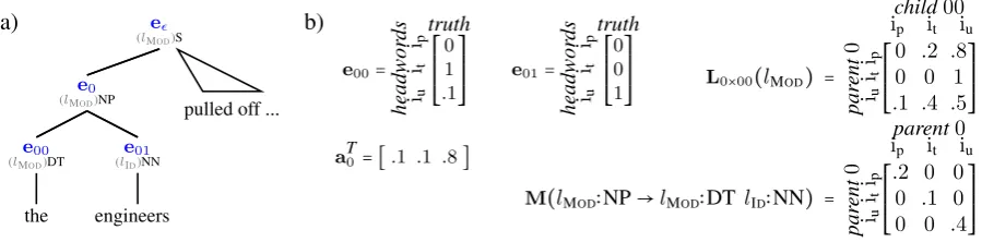
Figure 1: a) Syntax and semantics on a tree during decoding. Semantic vectorseare subscripted with the node’s address. Relationsland syntactic categoriescare constants for the example. b) Example vectors and matrices needed for the composition of a vector at address 0 (Section 2.2.1).

target vector are differentiated by subscript; instead of context variablesRandKwe will useM andL:

eγ=f(eα,eβ, M, L) (3)

Syntactic context is in the form of grammar rules M that are aware of semantic concepts; semantic knowledge is in the form of labeled dependency relationships between semantic concepts, L. Both of these are present and explicitly modeled as matrices in SVS’s canonical form of vector composition:

eγ=M⋅d(Lγ×α⋅eα)⋅d(Lγ×β⋅eβ)⋅1 (4)

Here,Mis a diagonal matrix that encapsulates probabilistic syntactic information, where the syntactic probabilities depend on the semantic concept being considered. TheLmatrices are linear transformations that capture how semantically relevant source vectors are to the resulting vector (e.g.,Lγ×α defines the

the relevance of e_α toe_γ), with the intuition that two 1D vectors are under consideration and require a 2D matrix to relate them. 1is a vector of ones — this takes a diagonal matrix and returns a column vector corresponding to the diagonal elements.

Of note in this definition of f(⋅) is the presence of matrices that operate on distributed semantic vectors. While it is widely understood that matrices can represent transformations, relatively few have used matrices to represent the distributed, dynamic nature of meaning composition (see Rudolph and Giesbrecht (2010) for a counterexample).

2.2 Syntax–Semantics Interface

This section aims to more thoroughly define the way in which the syntax and semantics interact during structured vectorial semantic composition. SVS will specify this interface such that the composition of semantic vectors is probabilistically consistent and subsumes parsing under various frameworks. Parsing has at times added semantic annotations that unwittingly carry some semantic value: headwords (Collins, 1997) are one-word concepts that subsume the words below them; latent annotations (Matsuzaki et al., 2005) are clustered concepts that touch on both syntactic and semantic information at a node. Of course, other annotations (Ge and Mooney, 2005) carry more explicit forms of semantics. In this light, semantic concepts (vector indices i) and relation labels (matrix argumentsl) may also be seen as annotations on grammar trees.

Let us introduce notation to make the connection with parsing and syntax explicit. This paper will denote syntactic categories ascand string yields asx. The location of these variables in phrase structure will be identified using subscripts that describe the path from the root to the constituent.1 Paths consist of left and/or right branches (indicated by ‘0’s and ‘1’s, respectively, as in Figure 1a). Variables α, β, andιstand for whole paths;γ is the path of a composed vector; andǫis the empty path at the root. The yieldxγis the observed (sub)string that eventually results from the progeny ofcγ. Multiple treesτγcan be constructed atγ by stringing together grammar rules that are consistent with observed text.

1

2.2.1 Lexicalized Parsing

To illustrate the definitions and operations presented in this section, we start with the concrete ‘semantic’ space of headwords (i.e., bilexical parsing) before moving on to a formal definition. Our example here corresponds to the best parse of the first two words in Figure 1a. In this example domain, assume that the semantic space of concept headwords is {ipulled,ithe,iunk}, abbreviated as {ip,it,iu} where the last concept is a constant for infrequently-observed words. This semantic space becomes the indices of semantic vectors; complete vectorseat each node of Figure 1a are shown in Figure 1b.

The tree in Figure 1a contains complete concept vectorseat each node, with corresponding indices

i. Values in these vectors (see Figure 1b) are probabilities, indicating the likelihood that a particular concept summarizes the meaning below a node. For example, considere00:itproduces the yield below address 00 (‘the’) with probability 1, andiumay also produce ‘the’ with probability 0.1.

Not shown on the tree are the matrices in Figure 1b. In the parametrized matrix

M(lMOD∶NP→lMOD∶DT lID∶NN), each diagonal element corresponds to the hypothesized grammar rule’s probability, given a headword. Similarly, the matrixL0_×00(lMOD)is parametrized by the semantic context lMOD — here,lMOD represents a generalized ‘modifier’ semantic role. For the semantic conceptipat ad-dress 0, the left-child modifier (adad-dress 00) could be semantic conceptitwith probability 0.2, or concept

iu with probability 0.8. Finally, by adding an identity matrix forL0_×01(lID)(a ‘head’ semantic role) to the quantities in Figure 1b, we would have all the components to construct the vector at address 0:

e0 = ⎡⎢ ⎢⎢ ⎢⎢ ⎣

.2 0 0

0 .1 0

0 0 .4

⎤⎥ ⎥⎥ ⎥⎥ ⎦ ´¹¹¹¹¹¹¹¹¹¹¹¹¹¹¹¹¹¹¹¸¹¹¹¹¹¹¹¹¹¹¹¹¹¹¹¹¹¹¹¶ M

⋅d⎛

⎝ ⎡⎢ ⎢⎢ ⎢⎢ ⎣

0 .2 .8 0 0 1

.1 .4 .5 ⎤⎥ ⎥⎥ ⎥⎥ ⎦ ´¹¹¹¹¹¹¹¹¹¹¹¹¹¹¹¹¹¹¹¸¹¹¹¹¹¹¹¹¹¹¹¹¹¹¹¹¹¹¹¶

L0_×01 ⎡⎢ ⎢⎢ ⎢⎢ ⎣ 0 1 .1 ⎤⎥ ⎥⎥ ⎥⎥ ⎦ ±_e 00 ⎞ ⎠⋅d

⎛ ⎝ ⎡⎢ ⎢⎢ ⎢⎢ ⎣

1 0 0 0 1 0 0 0 1 ⎤⎥ ⎥⎥ ⎥⎥ ⎦ ´¹¹¹¹¹¹¹¹¹¹¹¸¹¹¹¹¹¹¹¹¹¹¹¹¶ L0_×01

⎡⎢ ⎢⎢ ⎢⎢ ⎣ 0 0 1 ⎤⎥ ⎥⎥ ⎥⎥ ⎦ °_e 01 ⎞ ⎠⋅ ⎡⎢ ⎢⎢ ⎢⎢ ⎣ 1 1 1 ⎤⎥ ⎥⎥ ⎥⎥ ⎦ ° 1 = iu it ip truth ⎡⎢ ⎢⎢ ⎢⎢ ⎣ 0 0 0.036

⎤⎥ ⎥⎥ ⎥⎥ ⎦ ´¹¹¹¹¹¹¹¹¹¹¸¹¹¹¹¹¹¹¹¹¹¹¶_e 0

Since the vector was constructed in syntactic and semantic context, the tree structure shown (including semantic relationshipsl) is implied by the context.

2.2.2 Probabilities in vectors and matrices

Formally defining the probabilities in Figure 1, SVS populates vectors and matrices by means of 5 probability models (models are denoted byθ), along with the process of composition:

Syntactic model M(lcγ→lcαlcβ)[iγ, iγ]=PθM(lciγ→lcαlcβ)

Semantic model L_γ

×ι(lι)[iγ, iι]=PθL(iι∣iγ, lι)

Preterminal model e_γ[iγ]=PθP-Vit(G)(xγ∣lciγ), for pretermγ (5)

Root const. model aT_ǫ[iǫ]=PπGǫ(lciǫ)

Any const. model aT_γ[iγ]=PπG(lciγ)

These probabilities are encapsulated into vectors and matrices using a convention: column indices of vectors or matrices representconditionedsemantic variables, row indices representmodeledvariables.

As an example, from Figure 1b, elements ofL0_×00(lMOD)represent the probabilityPθL(i00∣i0, l00). Thus, the conditioned variable i00 is shown in the figure as column indices, and the modeled i0 as row indices. This convention applies to the M matrix as well. Recall that M is a diagonal matrix — its rows and columns model the same variable. Thus, we could rewrite PθM(lciγ → lcαlcβ) as PθM(lciγ→lcαlcβ, iγ)to make a consistent probabilistic interpretation.

We have intentionally left out the probabilistic definition of normal (non-preterminal) nonterminals PθVit(G), and the rationale fora

T_{vectors. These are both best understood in the dual problem of parsing.}

2.2.3 Vector Composition for Parsing

The vector composition of Equation 4 can be rewritten with all arguments and syntactic information as:

a compact representation that masks the underlying consistent probability operations. This section will expand the vector composition equation to show its equivalence to standard statistical parsing methods.

Let us say thateγ[iγ] = P(xγ∣lciγ), the probability of giving a particular yield given the present distributed semantics. Recall that in matrix multiplication, there is a summation over the inner dimen-sions of the multiplied objects; replacing matrices and vectors with their probabilistic interpretations and summing in the appropriate places, each element ofeγ is then:

eγ[iγ]=PθM(lciγ→lcαlcβ)⋅ ∑ iα

PθL(iα∣iγ, lα)⋅PθVit(G)(xα∣lciα) ⋅ ∑

iβ

PθL(iβ∣iγ, lβ)⋅PθVit(G)(xβ∣lciβ) (6)

This can be loosely considered the multiplication of the syntax (θM term), left-child semantics (first sum), and right-child semantics (second sum). The only summations are betweenLande, since all other multiplications are between diagonal matrices (similar to pointwise multiplication).

We can simplify this probability expression by grouping θM and θL into a grammar rule

PθG(lciγ→lciαlciβ)

def

=PθM(lciγ→lcαlcβ)⋅PθL(iα∣iγ, lα)⋅PθL(iβ∣iγ, lβ), since they deal with every-thing except the yield of the two child nodes. The summations are then pushed to the front:

eγ[iγ]= ∑ iα,iβ

PθG(lciγ→lciαlciβ)⋅PθVit(G)(xα∣lciα)⋅PθVit(G)(xβ∣lciβ) (7)

Thus, we have a standard chart-parsing probabilityP(xγ∣lciγ)— with distributed semantic concepts — in each vector element.

The use of grammar rules necessarily builds a hypothetical subtreeτγ. In a typical CKY algorithm, the tree corresponding to the highest probability would be chosen; however, we have not defined how to make this choice for vectorial semantics.

We will choose the best tree with probability 1.0, so we define a deterministic Viterbi probability over candidatevectors(not concepts) and context variables:

PθVit(G)(xγ∣lceγ)

def

=Jeγ=arg max

lce_ι (

aT_ιeι ⋅PπG(lca

T

ι)⋅PθVit(G)(x∣lceι))K (8)

whereJ⋅Kis an indicator function such thatJφK=1ifφis true,0otherwise. Intuitively, the process is as follows: we construct the vector e_ι at a node, according to Eqn. 4′_{; we then weight this vector against}

prior knowledge about the contextaT_ι; the best vector in context will be chosen (theargmax). Also, the vector at a node comes with assumptions of what structure produced it. Thus, the last two terms in the parentheses are deterministic models ensuring that the best subtreeτιis indeed the one generated.

Determining the root constituent of the Viterbi tree is the same process as choosing any other Viterbi constituent, except that prior contextual knowledge gets its own probability model in aT_ǫ. As before, the most likely tree τˆǫ is the tree that maximizes the probability at the root, and can be constructed recursively from the best child trees. Importantly,τˆǫhas an associated,sententialsemantic vector which may be construed as the composed semantic information for the whole parsed sentence. Similarphrasal semantic vectors can be obtained anywhere on the parse chart.

These equations complete the linear algebraic definition of structured vectorial semantics.

3

SVS with Relational Clusters

3.1 Inducing Relational Clusters

Let us re-notate the headword-lexicalized version of SVS (the example in Section 2.2.1) usingh

for headword semantics, and reserveifor relationally-clustered concepts. Treebank trees can be deter-ministically annotated with headwordsh and relationslby using head rules (Magerman, 1995). The 5 SVS modelsθM,θL,θP-Vit(G),πGǫ, andπGcan thus be obtained by counting instances and normalizing. Empirical probabilities of this kind are denoted with a tilde, whereas estimated models have a hat.

Conceptsiin a distributed semantic representation, however, cannot be found from annotated trees (see example concepts in Figure 2). Therefore, we use Expectation Maximization (EM) in a variant of the inside-outside algorithm (Baker, 1979) to learn distributed-concept behavior. In the M-step, the data-informed result of the E-step is used to update the estimates ofθM,θL, andθH(whereθHis a generlization ofθP-Vit(G)to any nonterminal). These updated estimates are then plugged back in to the next E-step. The two steps continually alternate until convergence or a maximum number of iterations.

E-step:

ˆ

P(iγ, iα, iβ∣lcγ, lcα, lcβ)=

ˆ

PθOut(lciγ, lchǫ−lchγ)⋅PˆθIns(lchγ∣lciγ) ˆ

P(lchǫ)

(9)

E(lciγ,lciα,lciβ)=Pˆ(iγ,iα,iβ∣lcγ,lcα,lcβ)⋅P˜(lcγ,lcα,lcβ)

M-step:

ˆ

PθM(lciγlcα, lcβ)=

∑iα,iβE(lciγ, lciα, lciβ)

∑lciα,lciβE(lciγ, lciα, lciβ)

ˆ

PθL(iα∣iγ;lα)=

∑lcγ,cα,lciβE(lciγ, lciα, lciβ)

∑lcγ,ciα,lciβE(lciγ, lciα, lciβ)

(10)

ˆ

PθH(hγ∣lciγ)=

E(lciγ,−,−)

∑hγE(lciγ,−,−)

Inside probabilities can be recursively calculated on training trees from the bottom up. These are simply probability sums of all subsumed subtrees (Viterbi probabilities with sums instead of maxes).

Outside probabilities can also be recursively calculated from training trees, here from parent proba-bilities. For a left child (the right-child case is similar):

ˆ

PθOut(lciα, lchǫ−lchα)=PˆθOut(lciγ, lchǫ−lchγ)⋅PˆθM(lciγlcα, lcβ) ⋅ ∑_iβPˆ_θ

L(iβ∣iγ, lβ)⋅PˆθIns(lchβ∣lciβ)⋅PˆθL(iα∣iγ, lα) (11)

Since outside probabilities signify everythingbutwhat is subsumed by the node, they carry a comple-mentary set of information to inside probabilities. Thus, inside and outside probabilities together are a natural way to produce parent and child clustered concepts.

3.2 Relational Semantic Clusters in Parsing

Section 2.2.2 listed the five probability models necessary for SVS. To define SVS with relational clusters, the estimates in Equation 10 can be used forθMandθL.

The preterminal model is based onθH, but it also includes some backoff for words that have not been used as headwords. The other two models also fall out nicely from the algorithm, though they are not explicitly estimated in EM. The prior probability at the root is just the base case for outside probabilities:

ˆ

PπGǫ(lciǫ)

def

=PˆθOut(lciǫ, lchǫ−lchǫ) (12)

Prior probabilities at non-root constituents are estimated from the empirically-weighted joint probability.

ˆ

PπG(lciγ)

def

= ∑

lciα,lciβ

˜

P(lciγ, lciα, lciβ) (13)

Clusteri1

‘announcement’

unk 0.362

was 0.173

reported 0.097 posted 0.036

earned 0.029

filed 0.024

were 0.022

had 0.020

told 0.013 approved 0.013

Clusteri5

‘change in value’

rose 0.137 fell 0.124

unk 0.116

gained 0.063 dropped 0.051 attributed 0.051 jumped 0.046 added 0.041 lost 0.039 advanced 0.022

Clusteri7

‘change possession’

unk 0.381

had 0.065

was 0.062

took 0.036 bought 0.027 completed 0.025 received 0.024

were 0.023

got 0.018 made 0.018 acquired 0.016

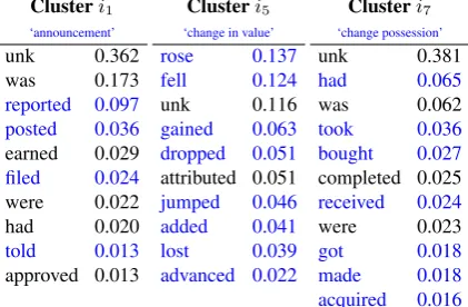
Figure 2: Example θH clusters from 1,000 head-words clustered into 10 referents, after 10 EM itera-tions, for transitive past-tense verbs (VBD-argNP).

0 5 10 15 20 25 30 35 40

0 100 200 300 400 500

Sentence Length

Average Parsing Time (s)

Non−vectorized Vectorized

Figure 3: Speed of relationally-clustered SVS parsers, with and without vectorization.

4

Evaluation

Sections 02–21 of the Wall Street Journal (WSJ) corpus were used as training data; Section 23 was used as test data with reported parsing results on sentences greater than length 40. Punctuation was left in for all reported evaluations. Trees were binarized, and syntactic states were thoroughly split into subcategorization classes. As previously discussed, unlike tests on of-the-art automatically state-splitting parsers, this isolates the contribution of semantics. The baseline 83.57 F-measure is comparable to Klein and Manning (2003) before the inclusion of head annotations.

Subsequently, each branch was annotated with a head relationlID or a modifier relationlMOD ac-cording to a binarized version of headword percolation rules (Magerman, 1995; Collins, 1997), and the headword was propagated up from its head constituent. The most frequent headwords (e.g.,h1, . . . , h50) were stored, and the rest were assigned a constant, ‘unk’ headword category.

From counts on the binary rules of these annotated trees, theθM, θL, θP-Vit(G), πGǫ, andπG proba-bilities for headword-lexicalization SVS were obtained. Modifier relationslMOD were deterministically augmented with their syntactic context; bothcandlsymbols appearing fewer than 10 times in the whole corpus were assigned ‘unknown’ categories.

These lexicalized models served as a baseline, but the augmented trees from which they were derived were also inputs to the EM algorithm in Section 3.1. Each parameter in the model or training algorithm was examined, with∣I∣={1,5,10,15,20}clusters, random initialization from reproducible seeds, and a varying numbers of EM iterations.

The implemented parser had few adjustments from a plain CKY parser other than these vectors. No approximate inference was used, with no beam for candidate parses and no re-ranking.

4.1 Interpretable relational clusters

Figure 2 shows example clusters for one of the headword models used, where EM clustered 1,000 head-words into 10 concepts in 10 iterations. The lists are parts of thePˆθH(hγ∣lciγ)model. As such, each of the 10 clusters will only produce headwords in light of some syntactic constituent. The figure shows how distributed concepts produce headwords for transitive past-tense verbs. Note that the probability distri-butions for different headwords are quite uneven, again confirming that some clusters are more specific, and others are more general.

a)

Sec. 23, length<40wds LR LP F

syntax-only baseline: 83.32 83.83 83.57

headword-lex. 10hw: 83.10 83.61 83.35

headword-lex. 50hw: 83.09 83.40 83.24

rel’n clust. 50hw10 clust: 83.67 84.13 83.90 b)

Sec. 23, length<40wds LR LP F

baseline1 clust 83.34 83.90 83.62

1000 hw5 clust, avg 83.85 84.23 84.04

1000 hw10 clust, avg 84.04 84.40 84.21 1000 hw15 clust, avg 84.15 84.38 84.26 1000 hw20 clust, avg 84.21 84.42 84.31

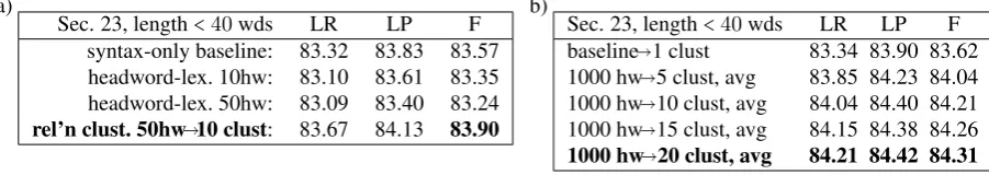
Table 1: a) Unsmoothed lexicalized CKY parsers versus 10 semantic clusters. Evaluations were run with EM trained to 10 iterations. b) Average dependence of parsing performance on number of semantic clusters. Averages are taken over different random seeds, with EM running 4 or 10 iterations.

4.2 Engineering considerations

We should note that relationally-clustered SVS is feasible with respect to random initialization and speed. Four relationally-clustered SVS models (with 500 headwords clustered into 5 concepts) were trained, each having a different random initialization. We found that the parsing F-score had a mean of 83.98 and a standard deviation of 0.21 across different initializations of the model. This indicates that though there are significant difference between the models, they still outperform models without SVS (see next section).

Also, it may seem slow to consider the set of semantic concepts and relations alongside syntax, at least with respect to normal parsing. The definition of SVS in terms of vectors actually mitigates this effect on WSJ Section 23, according to Figure 3. Since SVS is probabilistically consistent, the parser could be defined without vectors, but this would have the ‘non-vectorized’ speed curve. The contiguous storage and access of information in the ‘vectorized’ version leads to an efficient implementation.

4.3 Comparison to Lexicalization

One important comparison to draw here is between the effectiveness of semantic clusters versus headword-lexicalization. For fair head-to-head comparison on WSJ Section 23, both models were vector-ized and included no smoothing or backoff. Neither relational clusters nor lexicalization were optimvector-ized with backoff or smoothing.

Table 1a shows precision, recall, and F-score for lexicalized models and for clustered semantic mod-els. First, note that the 10-cluster model (in bold) improves on a syntax-only parser (top line), showing that the semantic model is contributing useful information to the parsing task.

Next, compare the 50-headword, 10-cluster model (in bold) to the line above it. It is natural to compare this model to the headword-lexicalized model with 50 headwords, since the same information from the trees is available to both models. The relationally-clustered model outperforms the headword-lexicalized model, showing that clustering the headwords actually improves their usefulness, despite the fact that fewer referents are used in the actual vectors.

It is also interesting, then, to compare this 50-headword, 10-cluster model to a headword-lexicalized model with 10 headwords. In this case, the possible size of the grammar is equal. Again, the relationally-clustered model outperforms plain lexicalization. This indicates that the 10 relationally-clustered referents are much more meaningful than 10 headword referents for the disambiguating of syntax.

4.4 Effect of Number of clusters

The final experiment on relational-clustering SVS was to determine whether performance would vary with the number of clusters. Table 1b compares average performance (over different random initializa-tions) for numbers of clusters from 1 (a syntax-equivalent case) to 20.

In addition, the table shows that average performance increases with the number of clusters. This loosely positive slope means that EM is still finding useful parts of the semantic space to explore and cluster, so that the clusters remain meaningful. However, the increase in performance with number of clusters is likely to eventually plateau.

Maximum-accuracy models were also evaluated, since each model is a full-fledged parser. The best 20-referent model obtained an F score of 84.60%, beating the syntactic baseline by almost a full absolute point. Thus, finding relationally-clustered semantic output also contributes to some significant parsing benefit.

4.5 Perplexity

Finally, per-word perplexities were calculated for a syntactic model and for a 5-concept relationally-clustered model. Specific to this evaluation, following Mitchell and Lapata (2009), only the top 20,000 words in WSJ Sections 02-21 were kept in training or test sentences, and the rest replaced with ‘unk’; numbers were replaced with ‘num.’

Sec. 23, ‘unk’+‘num’ Perplexity

syntax only baseline 428.94

rel’n clust. 1khw→005e 371.76

Table 2: Model fit as measured by perplexity.

Table 2 shows that adding semantic information greatly reduces perplexity. Since as much syntactic information as possible (such as argument structure) has been pre-annotated onto trees, the isolated contribution of interactive semantics improves on a syntax-only model model.

5

Conclusion

This paper has introduced a structured vectorial semantic (SVS) framework in which vector composition and syntactic parsing are a single, interactive process. The framework thus fully integrates distributional semantics with traditional syntactic models of language.

Two standard parsing techniques were defined within SVS and evaluated: headword-lexicalization SVS (bilexical parsing) and relational-clustering SVS (latent annotations). It was found that relationally-clustered SVS outperformed the simpler lexicalized model and syntax-only models, and that additional clusters had a mildly positive effect. Additionally, perplexity results showed that the integration of distributed semantics in relationally-clustered SVS improved the model over a non-interactive baseline.

It is hoped that this flexible framework will enable new generations of interactive interpretation models that deal with the syntax–semantics interface in a plausible manner.

References

Baker, J. (1979). Trainable grammars for speech recognition. In D. Klatt and J. Wolf (Eds.), Speech Communication Papers for the 97th Meeting of the Acoustical Society of America, pp. 547–550.

Blei, D. M., A. Y. Ng, and M. I. Jordan (2003). Latent dirichlet allocation. Journal of Machine Learning Research 3, 993–1022.

Charniak, E. (1996). Tree-bank grammars. In Proceedings of the National Conference on Artificial Intelligence, pp. 1031–1036.

Deerwester, S., S. Dumais, G. W. Furnas, T. K. Landauer, and R. Harshman (1990). Indexing by latent semantic analysis. Journal of the American Society for Information Science 41(6), 391–407.

Erk, K. and S. Pad´o (2008). A structured vector space model for word meaning in context. InProceedings of EMNLP 2008.

Frege, G. (1892). Uber sinn und bedeutung. Zeitschrift fur Philosophie und Philosophischekritik 100, 25–50.

Ge, R. and R. J. Mooney (2005). A statistical semantic parser that integrates syntax and semantics. In Ninth Conference on Computational Natural Language Learning, pp. 9–16.

Gesmundo, A., J. Henderson, P. Merlo, and I. Titov (2009). A latent variable model of synchronous syntactic-semantic parsing for multiple languages. InProceedings of CoNLL, pp. 37–42. Association for Computational Linguistics.

Griffiths, T. L., M. Steyvers, D. M. Blei, and J. B. Tenenbaum (2005). Integrating topics and syntax. Advances in neural information processing systems 17, 537–544.

Hofmann, T. (2001). Unsupervised learning by probabilistic latent semantic analysis. Machine Learn-ing 42(1), 177–196.

Klein, D. and C. D. Manning (2003). Accurate unlexicalized parsing. InProceedings of the 41st Annual Meeting of the Association for Computational Linguistics, Sapporo, Japan, pp. 423–430.

Koo, T., X. Carreras, and M. Collins (2008). Simple semi-supervised dependency parsing. In Proceed-ings of the 46th Annual Meeting of the ACL, Volume 8. Citeseer.

Lin, D. (1998). An information-theoretic definition of similarity. InProceedings of the 15th International Conference on Machine Learning, Volume 296304.

MacDonald, M. C., N. J. Pearlmutter, and M. S. Seidenberg (1994). The lexical nature of syntactic ambiguity resolution. Psychological Review 101(4), 676–703.

Magerman, D. (1995). Statistical decision-tree models for parsing. InProceedings of the 33rd Annual Meeting of the Association for Computational Linguistics (ACL’95), Cambridge, MA, pp. 276–283.

Matsuzaki, T., Y. Miyao, and J. Tsujii (2005). Probabilistic CFG with latent annotations. InProceedings of the 43rd Annual Meeting on Association for Computational Linguistics, pp. 75–82. Association for Computational Linguistics.

Mitchell, J. and M. Lapata (2008). Vector-based models of semantic composition. In Proceedings of ACL-08: HLT, Columbus, OH, pp. 236–244.

Mitchell, J. and M. Lapata (2009). Language Models Based on Semantic Composition. InProceedings of the 2009 Conference on Empirical Methods in Natural Language Processing, pp. 430–439.

Pad´o, S. and M. Lapata (2007). Dependency-based construction of semantic space models. Computa-tional Linguistics 33(2), 161–199.

Petrov, S., L. Barrett, R. Thibaux, and D. Klein (2006). Learning accurate, compact, and interpretable tree annotation. In Proceedings of the 44th Annual Meeting of the Association for Computational Linguistics (COLING/ACL’06).

Rudolph, S. and E. Giesbrecht (2010). Compositional matrix-space models of language. InProceedings of ACL 2010. Association for Computational Linguistics.