On Semi Supervised Learning of Gaussian Mixture Models for Phonetic Classification

On Semi-Supervised Learning of Gaussian Mixture Models

for Phonetic Classification

Jui-Ting Huang and Mark Hasegawa-Johnson Department of Electrical and Computer Engineering

University of Illinois at Urbana-Champaign Illinois, IL 61801, USA

{jhuang29,jhasegaw_}@illinois.edu

Abstract

This paper investigates semi-supervised learn-ing of Gaussian mixture models uslearn-ing an uni-fied objective function taking both labeled and unlabeled data into account. Two methods are compared in this work – the hybrid dis-criminative/generative method and the purely generative method. They differ in the crite-rion type on labeled data; the hybrid method uses the class posterior probabilities and the purely generative method uses the data like-lihood. We conducted experiments on the TIMIT database and a standard synthetic data set from UCI Machine Learning repository. The results show that the two methods be-have similarly in various conditions. For both methods, unlabeled data improve training on models of higher complexity in which the su-pervised method performs poorly. In addition, there is a trend that more unlabeled data re-sults in more improvement in classification ac-curacy over the supervised model. We also provided experimental observations on the rel-ative weights of labeled and unlabeled parts of the training objective and suggested a criti-cal value which could be useful for selecting a good weighing factor.

1 Introduction

Speech recognition acoustic models can be trained using untranscribed speech data (Wessel and Ney, 2005; Lamel et al., 2002; L. Wang and Woodland, 2007). Most such experiments begin by boostraping

∗_{This research is funded by NSF grants 0534106 and}

0703624.

an initial acoustic model using a limited amount of manually transcribed data (normally in a scale from 30 minutes to several hours), and then the initial model is used to transcribe a relatively large amount of untranscribed data. Only the transcriptions with high confidence measures (Wessel and Ney, 2005; L. Wang and Woodland, 2007) or high agreement with closed captions (Lamel et al., 2002) are se-lected to augment the manually transcribed data, and new acoustic models are trained on the augmented data set.

The general procedure described above exactly lies in the context of semi-supervised learning prob-lems and can be categorized as a self-training algo-rithm. Self-training is probably the simplest semi-supervised learning method, but it is also flexible to be applied to complex classifiers such as speech recognition systems. This may be the reason why little work has been done on exploiting other semi-supervised learning methods in speech recognition. Though not incorporated to speech recognizers yet, there has been some work on semi-supervised learn-ing of Hidden Markov Models (HMM) for sequen-tial classification. Inoue and Ueda (2003) treated the unknown class labels of the unlabeled data as hidden variables and used the expectation-maximization (EM) algorithm to optimize the joint likelihood of labeled and unlabeled data. Recently Ji et al. (2009) applied a homotopy method to select the optimal weight to balance between the log likelihood of la-beled and unlala-beled data when training HMMs.

the transcriptions are available. Wang and Wood-land (2007) used the self-training method to aug-ment the training set for discriminative training. Huang and Hasegawa-Johnson (2008) investigated another use of discriminative information from la-beled data by replacing the likelihood of lala-beled data with the class posterior probability of labeled data in the semi-supervised training objective for Gaussian Mixture Models (GMM), resulting in a hybrid dis-criminative/generative objective function. Their ex-perimental results in binary phonetic classification showed significant improvement in classification ac-curacy when labeled data are scarce. A similar strat-egy called ”‘multi-conditional learning”’ was pre-sented in (Druck et al., 2007) applied to Markov Random Field models for text classification tasks, with the difference that the likelihood of labeled data is also included in the objective. The hybrid dis-criminative/generative objective function can be in-terpreted as having an extra regularization term, the likelihood of unlabeled data, in the discriminative training criterion for labeled data. However, both methods in (Huang and Hasegawa-Johnson, 2008) and (Druck et al., 2007) encountered the same issue about determining the weights for labeled and un-labeled part in the objective function and chose to use a development set to select the optimal weight. This paper provides an experimental analysis on the effect of the weight.

With the ultimate goal of applying semi-supervised learning in speech recognition, this pa-per investigates the learning capability of algorithms within Gaussian Mixture Models because GMM is the basic model inside a HMM, therefore 1) the up-date equations derived for the parameters of GMM can be conveniently extended to HMM for speech recognition. 2) GMM can serve as an initial point to help us understand more details about the semi-supervised learning process of spectral features.

This paper makes the following contribution:

• it provides an experimental comparison of hy-brid and purely generative training objectives.

• it studies the impact of model complexity on learning capability of algorithms.

• it studies the impact of the amount of unlabeled data on learning capability of algorithms.

• it analyzes the role of the relative weights of labeled and unlabeled parts of the training ob-jective.

2 Algorithm

Suppose a labeled set_XL= (x1, . . . , xn, . . . , xNL)

has NL data points and xn ∈ Rd. YL = (y1, . . . , yn, . . . , yNL) are the corresponding class

labels, whereyn∈ {1,2, . . . , Y}and Y is the

num-ber of classes. In addition, we also have an unla-beled setXU =(x1, . . . , xn, . . . , xNU) without

cor-responding class labels. Each class is assigned a Gaussian Mixture model, and all models are trained given XL and XU. This section first presents the

hybrid discriminative/generative objective function for training and then the purely generative objective function. The parameter update equations are also derived here.

2.1 Hybrid Objective Function

The hybrid discriminative/generative objective func-tion combines the discriminative criterion for la-beled data and the generative criterion for unlala-beled data:

F(λ) = logP(YL|XL;λ) +αlogP(XU;λ), (1)

and we chose the parameters so that (1) is maxi-mized:

ˆ

λ= arg max

λ F(λ). (2)

The first component considers the log posterior class probability of the labeled set whereas the sec-ond component considers the log likelihood of the unlabeled set weighted byα. In ASR community, model training based the first component is usually referred to as Maximum Mutual Information Esti-mation (MMIE) and the second component Maxi-mum Likelihood Estimation (MLE), therefore in this paper we use a brief notation for (1) just for conve-nience:

F(λ) =F(DL)

MMI (λ) +αF

(DU)

ML (λ). (3)

scales of the posterior probability and the likeli-hood are essentially different, so are their gradients. While the weight α balances the impacts of two components on the training process, it may also im-plicitly normalize the scales of the two components. In section (3.2) we will discuss and provide a further experimental analysis.

In this paper, the models to be trained are Gaus-sian mixture models of continuous spectral feature vectors for phonetic classes, which can be further extended to Hidden Markov Models with extra pa-rameters such as transition probabilities.

The maximization of (1) follows the techniques in (Povey, 2003), which uses auxiliary functions for objective maximization; In each iteration, a strong or weak sense auxiliary function is maximized, such that if the auxiliary function converges after itera-tions, the objective function will be at a local maxi-mum as well.

The objective function (1) can be rewritten as

F(λ) = logP(XL|YL;λ)−logP (XL;λ) +αlogP (_XU;λ),

(4)

where the termlogP (_YL;λ)is removed because it is independent of acoustic model parameters.

The auxiliary function at the current parameter λold_{for (4) is}

G(λ, λ(old)_{) =G}num_{(λ, λ}(old)_{)− G}den_{(λ, λ}(old)₎

+αGden_{(λ, λ}(old)_;D

U) +Gsm(λ, λ(old)),

(5)

where the first three terms are strong-sense auxiliary functions for the conditional likelihood (referred to as the numerator(num) model because it appears in the numerator when computing the class posterior probability)logP (XL|YL;λ)and the marginal

like-lihoods (referred to as the denominator(den) model likewise)logP (XL;λ)andαlogP(XU;λ)

respec-tively. The last term is a smoothing function that doesn’t affect the local differential but ensures that the sum of the first three term is at least a convex weak-sense auxiliary function for good convergence in optimization.

Maximization of (5) leads to the update equations

for the classjand mixturemgiven as follows:

ˆ

µjm= 1

γ_jm xxx num

jm,−xxxdenjm+αxxxdenjm(DU) +Djmµjm

(6)

ˆ

σ2_jm= 1 γ_jm sss

num

jm −sssdenjm+αsssdenjm(DU)

+Djm σ2jm+µ2jm

−µˆ2_jm, (7)

where for clarity the following substitution is used:

γ_jm=γ_jmnum−γ_jmden+αγ_jmden(DU) +Djm (8)

andγjm is the sum of the posterior probabilities of

occupation of mixture componentmof classjover the dataset:

γnum jm (X) =

X

xi∈X,yi=j

p(m_|xi, yi=j)

γ_jmden(X) = X

xi∈X

p(m_|xi)

(9)

and xxxjm and sssjm are respectively the weighted

sum of xi and x2i over the whole dataset with the

weightp(m_|xi, yi =j) or p(m|xi), depending on

whether the superscript is the numerator or denomi-nator model. Djmis a constant set to be the greater

of twice the smallest value that guarantees positive variances orγden

jm (Povey, 2003). The re-estimation

formula for mixture weights is also derived from the Extended Baum-Welch algorithm:

ˆ

cjm=

cjm n

∂F

∂cjm +C o

P m′cjm′

n ∂F

∂cjm +C

o, (10)

where the derivative was approximated (Merialdo, 1988) in the following form for practical robustness for small-valued parameters :

∂FMMI ∂cjm ≈

γnum jm P

m′γ_jmnum′ − γden

jm P

m′γ_jmden′

. (11)

Under our hybrid framework, there is an extra term γden

jm(DU)/Pm′γ_jmden′(DU)that should exist in (11),

2.2 Purely Generative Objective

In this paper we compare the hybrid objective with the purely generative one:

F(λ) = logP(_XL|YL;λ) +αlogP (XU;λ),

(12) where the two components are total log likelihood of labeled and unlabeled data respectively. (12) doesn’t suffer from the problem of combining two heteroge-neous probabilistic items, and the weight α being equal to one means that the objective is a joint data likelihood of labeled and unlabeled set with the as-sumption that the two sets are independent. How-ever, DL or DU might just be a sampled set of the

population and might not reflect the true proportion, so we keepαto allow a flexible combination of two criteria. On top of that, we need to adjust the relative weights of the two components in practical experi-ments.

The parameter update equation is a reduced form of the equations in Section (2.1):

ˆ

µjm=

x xxnum

jm,+αxxxdenjm(DU)

γnum

jm +αγjmden(DU)

(13)

ˆ

σ_jm2 = sss num

jm +αsssdenjm(DU)

γnum

jm +αγjmden(DU)

−µˆ2_jm (14)

3 Results and Discussion

The purpose of designing the learning algorithms is for classification/recognition of speech sounds, so we conducted phonetic classification experiments using the TIMIT database (Garofolo et al., 1993). We would like to investigate the relation of learning capability of semi-supervised algorithms to other factors and generalize our observations to other data sets. Therefore, we used another synthetic dataset

Waveform for the evaluation of semi-supervised learning algorithms for Gaussian Mixture model.

TIMIT: We used the same 48 phone classes and further grouped into 39 classes according to (Lee and Hon, 1989) as our final set of phone classes to model. We extracted 50 speakers out of the NIST complete test set to form the development set. All of our experimental analyses were on the develop-ment set. We used segdevelop-mental features (Halberstadt, 1998) in the phonetic classification task. For each

phone occurrence, a fixed-length vector was calcu-lated from the frame-based spectral features (12 PLP coefficients plus energy) with a5ms frame rate and a25 ms Hamming window. More specifically, we divided the frames for each phone into three regions with 3-4-3 proportion and calculated the PLP av-erage over each region. Three averages plus the log duration of that phone gave a 40-dimensional (13×3 + 1) measurement vector.

Waveform: We used the second versions of the Waveform dataset available at the UCI reposi-tory (Asuncion and Newman, 2007). There are three classes of data. Each token is described by 40 real attributes, and the class distribution is even.

Forwaveform, because the class labels are equally distributed, we simply assigned equal number of mixtures for each class. For TIMIT, the phone classes are unevenly distributed, so we assigned variable number of Gaussian mixtures for each class by controlling the averaged data counts per mixture. For all experiments, the initial model is an MLE model trained with labeled data only.

To construct a mixed labeled/unlabeled data set, the original training set were randomly divided into the labeled and unlabeled sets with desired ratio, and the class labels in the unlabeled set are assumed to be unknown. To avoid that the classifier performance may vary with particular portions of data, we ranfive

folds for every experiment, each fold corresponding to different division of training data into labeled and unlabeled set, and took the averaged performance.

3.1 Model Complexity

This section analyzes the learning capability of semi-supervised learning algorithms for different model complexities, that is, the number of mix-tures for Gaussian mixture model. In this experi-ment, the sizes of labeled and unlabeled set are fixed (_|DL| : |DU| = 1 : 10 and the averaged token

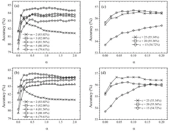
accura-Figure 1: Mean classification accuracies vs. αfor different model complexity. The accuracies for the initial MLE models are indicated in the parentheses. (a)waveform: training with the hybrid objective. (b)waveform: purely generative objective. (c) TIMIT: training with the hybrid objective. (d) TIMIT: purely generative objective.

! !" #! #!" $!

%& ' '# '$ '( ') '"

!"

!

"

"

#$

%

"

&

'

(

)

#$#%#&# '()*&+"

#$#%#(# '&)*'+"

#$#%#,# '-)./+"

#$#%#.# '*)-'+"

#$#%#/# 01)/-+"

2"

! ! " !# !#" !$

"( ") "" "* "% 3"

#

!

"

"

#$

%

"

&

'

(

)

#3#%#&.# ..)(,+"

#3#%#&*# ..)(/+"

#3##%#-.# .,)0&+"

! !" #! #!" $!

%& ' '# '$ '( ') '"

4"

#

!

"

"

#$

%

"

&

'

(

)

#

#$#%#&# '()*&+"

#$#%#(# '&)*'+"

#$#%#,# '-)./+"

#$#%#.# '*)-'+"

#$#%#/# 01)/-+"

! ! " !# !#" !$

"( ") "" "* "%

#

#

!

"

"

#$

%

"

&

'

(

)

#3#%#&.# ..)(,+"

#3#%#&*# ..)(/+"

#3#%#-.# .,)0&+"

cies of the updated model versus the value ofαwith different model complexities. The ranges ofα are different forwaveformand TIMIT because the value ofαfor each dataset has different scales.

First of all, the hybrid method and purely gen-erative method have very similar behaviors in both

waveform and TIMIT; the differences between the two methods are insignificant regardless ofα. The hybrid method withα = 0means supervised MMI-training with labeled data only, and the purely gener-ative method withα= 0means extra several rounds of supervised MLE-training if the convergence cri-terion is not achieved. With the small amount of la-beled data, most of hybrid curves start slightly lower than the purely generative ones at α = 0, but in-crease to as high as the purely generative ones asα increases.

Forwaveform, the accuracies increase withα in-creases for all cases except for the 2-mixture model. Table 1 summarizes the numbers from Figure 3.1.

Except for the 2-mixture case, the improvement over the supervised model (α = 0) is positively corre-lated to the model complexity, as the largest im-provements occur at the 5-mixture and 6-mixture model for the hybrid and purely generative method respectively. However, the highest complexity does not necessarily gives the best classification racy; the 3-mixture model achieves the best accu-racy among all models after semi-supervised learn-ing whereas the 2-mixture model is the best model for supervised learning using labeled data only.

Experiments on TIMIT show a similar behavior1; as shown in both Figure 3.1 and Table 2, the im-provement over the supervised model (α = 0) is also positively correlated to the model complexity,

1

Table 1: The accuracies(%) of the initial MLE model, the supervised model (α= 0), the best accuracies with unlabeled data and the absolute improvements (∆) overα = 0for different model complexities for waveform. The bolded number is the highest value along the same column.

Hybrid Purely generative #. mix init. acc. α= 0 best acc. ∆ α= 0 best acc. ∆

2 83.02 81.73 83.74 2.01 82.96 83.14 0.18

3 82.08 81.66 84.69 3.03 82.18 84.58 2.40 4 81.56 80.53 83.93 3.40 81.34 84.13 2.79 5 80.18 80.14 83.82 3.68 80.16 83.84 3.68 6 79.61 79.40 83.19 3.79 79.71 83.31 3.60

Table 2: The accuracies(%) of the initial MLE model, the supervised model (α= 0), the best accuracies with unlabeled data and the absolute improvements (∆) overα= 0for different model complexities for TIMIT. The bolded number is the highest value along the same column.

Hybrid Purely generative c init. acc. α= 0 best acc. ∆ α= 0 best acc. ∆ 25 55.34 55.47 56.58 1.11 55.32 56.7 1.38

20 55.36 55.67 56.72 1.05 55.2 56.25 1.05

15 54.72 53.71 55.39 1.68 53.7 56.09 2.39

as the most improvements occur atc = 25for both hybrid and purely generative methods. The semi-supervised model consistently improves over the su-pervised model. To summarize, unlabeled data im-prove training on models of higher complexity, and sometimes it helps achieve the best performance with a more complex model.

3.2 Size of Unlabeled Data

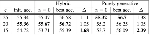
In Figure 2, we fixed the size of the labeled set (4% of the training set) and plotted the averaged classi-fication accuracies for learning with different sizes of unlabeled data. First of all, the hybrid method and purely generative method still behave similarly in bothwaveformand TIMIT. For both datasets, the figures clearly illustrate that more unlabeled data contributes more improvement over the supervised model regardless of the value ofα. Generally, a data distribution can be expected more precisely with a larger sample size from the data pool, therefore we expect the more unlabeled data the more precise in-formation about the population, which improves the learning capability.

3.3 Discussion ofα

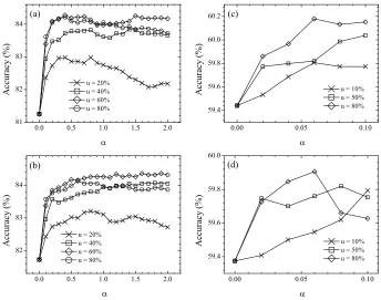
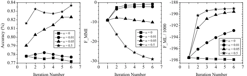
During training, the weighted sum of_FMMIandFML

in equation (15) increases with iterations, however FMMIand FMLare not guaranteed to increase

indi-vidually. Figure 3 illustrates howα affects the re-spective change of the two components for a partic-ular setting for waveform. When α = 0, the ob-jective function does not take unlabeled data into account, soFMMI increases while FML decreases. FML starts to increase for nonzero α; α = 0.01

corresponds to the case where both objectives in-creases. As α keeps growing, FMMI starts to

de-crease whereas FML keeps rising. In this

partic-ular example, α = 0.05 is the critical value at which _FMMI changes from increasing to

normal-Figure 2: Mean classification accuracies vs. αfor different amounts of unlabeled data (the percentage in the training set). The averaged accuracy for the initial MLE model is81.66%forwaveformand59.41%for TIMIT. (a)waveform: training with the hybrid objective. (b)waveform: purely generative objective. (c) TIMIT: training with the hybrid objective. (d) TIMIT: purely generative objective.

! !" #! #!" $!

%# %$ %& %'

!

"

"

#$

%

"

&

'

(

)

! " #$%

! " &$%

! " '$%

! " ($%

! ! " !#

"(!' "(!) "(!% ) ! ) !$

!

"

"

#$

%

"

&

'

(

)

! " )$%

! " *$%

! " ($%

! !" #! #!" $!

%$ %& %'

!

"

"

#$

%

"

&

'

(

)

! " #$%

! " &$%

! " '$%

! " ($%

! ! " !#

"(!' "(!) "(!% ) !

!

"

"

#$

%

"

&

'

(

)

! " )$%

! " *$%

! " ($%

+,-

+.-

+/-

+0-ization factor with respect to the relative size of la-beled/unlabeled set. The objective function in (15) can be rewritten in terms of the normalized objective with respect to the data size:

F(λ) =_|DL|F(MMIDL)(λ) +α|DU|F(MLDU)(λ). (15)

where_F(X)means the averaged value over the data setX. When the labeled set size increases, αmay have to scale up accordingly such that the relative change of the two averaged component remains in the same scale.

Although α controls the dominance of the crite-rion on labeled data or on unlabeled data, the fact that which dominates the objective or the critical value does not necessary indicate the bestα. How-ever, we observed that the bestαis usually close to or larger than the critical value, but the exact value varies with different data. At this point, it might still

be easier to find the best weight using a small de-velopment set. But this observation also provides a guide about the reasonable range to search the best α– searching starting from the critical value and it should reach the optimal value soon according to the plots in Figure 3.1.

Table 3: The critical values for waveform and TIMIT for different sizes of labeled data (percentage of training data) with a fixed set of unlabeled data (80 %.)

Figure 3: Accuracy (left),FMMI(center), andFML(right) at different values ofalpha.

! " # $ % & ' (''

(') ('* () ()! ()" ()# ()$

!

"

"

#

$

%

"

&

'

(

)

!"#$!%&'()*+,"#

((-(.

((-(./.0 ((-(./.1

((-(./1

! " # $ % & ' +#

+" +!

*

+

,

,

!"#$!%&'()*+,"#

((-(.

((-(./.0 ((-(./.1

((-(./1

! " # $ % & ' +!*)

+!*& +!*$ +!*" +!* +!))

*

+

,

.

/

0

1

1

1

!"#$!%&'()*+,"#

((-(. ((-(./.0

((-(./.1

((-(./1

3.4 Hybrid Criterion vs. Purely Generative Criterion

From the previous experiments, we found that the hybrid criterion and purely generative criterion al-most match each other in performance and are able to learn models of the same complexity. This implies that the criterion on labeled data has less impact on the overall training direction than unlabeled data. In Section 3.2, we mentioned that the bestαis usually larger than or close to the critical value around which the unlabeled data likelihood tends to dominate the training objective. This again suggests that labeled data contribute less to the training objective function compared to unlabeled data, and the criterion on la-beled data doesn’t matter as much as the criterion on unlabeled data. It is possible that most of the con-tributions from labeled data have already been used for training an initial MLE model, therefore little in-formation could be extracted in the further training process.

4 Conclusion

Regardless of the dataset and the training objective type on labeled data, there are some general prop-erties about the semi-supervised learning algorithms studied in this work. First, while limited amount of labeled data can at most train models of lower com-plexity well, the addition of unlabeled data makes the updated models of higher complexity much im-proved and sometimes perform better than less

com-plex models. Second, the amount of unlabeled data in our semi-supervised framework generally follows ‘the-more-the-better’ principle; there is a trend that more unlabeled data results in more improvement in classification accuracy over the supervised model.

We also found that the objective type on labeled data has little impact on the updated model, in the sense that hybrid and purely generative objectives behave similarly in learning capability. The obser-vation that the bestαoccurs after the MMI criterion begins to decrease supports the fact that the criterion on labeled data contributes less than the criterion on unlabeled data. This observation is also helpful in determining the search range for the bestα on the development set by locating the critical value of the objective as a start point to perform search.

References

A. Asuncion and D.J. Newman. 2007. UCI machine learning repository.

Gregory Druck, Chris Pal, Andrew McCallum, and Xiao-jin Zhu. 2007. Semi-supervised classification with hy-brid generative/discriminative methods. InKDD ’07: Proceedings of the 13th ACM SIGKDD international

conference on Knowledge discovery and data mining,

pages 280–289, New York, NY, USA. ACM.

J. S. Garofolo, L. F. Lamel, W. M. Fisher, J. G. Fiscus, D. S. Pallett, and N. L. Dahlgren. 1993. Darpa timit acoustic phonetic continuous speech corpus.

Andrew K. Halberstadt. 1998. Heterogeneous Acous-tic Measurements and Multiple Classifiers for Speech

Recognition. Ph.D. thesis, Massachusetts Institute of

Technology.

J.-T. Huang and Mark Hasegawa-Johnson. 2008. Max-imum mutual information estimation with unlabeled data for phonetic classification. InInterspeech. Masashi Inoue and Naonori Ueda. 2003. Exploitation of

unlabeled sequences in hidden markov models. IEEE

Trans. On Pattern Analysis and Machine Intelligence,

25:1570–1581.

Shihao Ji, Layne T. Watson, and Lawrence Carin. 2009. Semisupervised learning of hidden markov models via a homotopy method.IEEE Trans. Pattern Anal. Mach.

Intell., 31(2):275–287.

M.J.F. Gales L. Wang and P.C. Woodland. 2007. Un-supervised training for mandarin broadcast news and conversation transcription. In Proc. IEEE Confer-ence on Acoustics, Speech, and Signal Processing

(ICASSP), volume 4, pages 353–356.

Lori Lamel, Jean-Luc Gauvain, and Gilles Adda. 2002. Lightly supervised and unsupervised acoustic model training. 16:115–129.

K.-F. Lee and H.-W. Hon. 1989. Speaker-independent phone recognition using hidden markov models.

IEEE Transactions on Speech and Audio Processing,

37(11):1641–1648.

B. Merialdo. 1988. Phonetic recognition using hid-den markov models and maximum mutualinformation training. In Proc. IEEE Conference on Acoustics,

Speech, and Signal Processing (ICASSP), volume 1,

pages 111–114.

Daniel Povey. 2003. Discriminative Training for Large

Vocabulary Speech Recognition. Ph.D. thesis,

Cam-bridge University.

Fei Sha and Lawrence K. Saul. 2007. Large margin hid-den markov models for automatic speech recognition. In B. Sch¨olkopf, J. Platt, and T. Hoffman, editors,

Ad-vances in Neural Information Processing Systems 19,

pages 1249–1256. MIT Press, Cambridge, MA.

Frank Wessel and Hermann Ney. 2005. Unsupervised training of acoustic models for large vocabulary con-tinuous speech recognition. IEEE Transactions on