A recursive method for solving a climate economy model: value function iterations with logarithmic approximations

Munich Personal RePEc Archive

A recursive method for solving a

climate-economy model: value function

iterations with logarithmic

approximations

Hwang, In Chang

25 March 2014

Online at

https://mpra.ub.uni-muenchen.de/54782/

A recursive method for solving a climate-economy model: value function iterations with

logarithmic approximations

In Chang Hwang

VU University Amsterdam, Institute for Environmental Studies, Amsterdam, The

Netherlands, De Boelelaan 1087, Amsterdam, The Netherlands, 1081 HV, Tel.: +31 6 1602

5459, E-mail: [email protected]

Abstract

A recursive method for solving an integrated assessment model of climate and the economy

is developed in this paper. The method approximates value function with a logarithmic basis

function and searches for solutions on a set satisfying optimality conditions. These features

make the method suitable for a highly nonlinear model with many state variables and various

constraints, as usual in a climate-economy model.

Key words

Dynamic programming; recursive method; value function iteration; integrated assessment

JEL Classification

1 Introduction

This paper develops a numerical method for solving a climate economy model. Since an

integrated assessment model (IAM) of climate and the economy is highly nonlinear and is

subject to various constraints, it is not possible to solve the model analytically. Nonlinear

programming has been usually applied for numerically solving IAMs. For instance the DICE

2007 model (Nordhaus, 2008) is solved with CONOPT (nonlinear programming) in GAMS

modelling system. However the need for solving an IAM recursively (e.g., solving the

Bellman equation) is growing because it helps investigate the effect of uncertainty and

learning on policy and welfare (e.g., Kelly and Kolstad, 1999).

The method of this paper is suitable for this kind of numerical analysis because it is less

prone to the number of state variables than the existing methods in the literature. The main

advantage of the method of this paper is that it is simple and transparent because it obtains

solutions from optimality conditions. The disadvantage is that one should specify the first

order conditions analytically, which may require tedious calculations if the number of state

variables and control variables becomes large.

In most dynamic programming literature solving an IAM, the problem is reformulated in a

recursive way and the value function is approximated to a flexible basis function. Then the

fixed-point theorem is applied to find solutions.1 One of the main differences among existing

papers is the approximation method. For instance, Kelly and Kolstad (1999) and Leach (2007)

use neural networks approximations, Kelly and Tan (2013) apply spline approximations, and

1

See Bellman and Dreyfus (1962), Stokey and Lucas (1989), Rust (1996), Judd (1998), and Miranda and

Cai et al. (2012b) and Lemoine and Traeger (2014) apply Chebyshev polynomials

approximations. A basis function is useful in that it has an analytical functional form.

A dynamic climate-economy model is not generally time autonomous since it has many

exogenous variables such as labor force and technology. To address this issue, Kelly and

Kolstad (1999), Leach (2007), and Lemoine and Traeger (2014) add time as an argument for

the value function. Cai et al. (2012b) let the coefficients of the basis function vary each time

period. Kelly and Tan (2013) make the model time independent.

This paper presents a different method from the literature: logarithmic approximations.

Exogenous variables can be added as arguments for the basis function in order to address the

problem of time dependence, but whether or not exogenous variables are added does not

affect the accuracy of the method. In addition, the solution method of this paper differs from

the literature in that it searches for solutions on an ergodic set, whereas the other papers

generally search for solutions on a carefully designed grid. A grid based method is generally

prone to the ‘curse of dimensionality’ (for more discussion, see Judd et al., 2011). For

instance, DICE has 2 control variables, 6 endogenous state variables, and 9 (time-dependent)

exogenous variables. Thus, the number of the total grid points will be n7, if we apply a grid based method with n grid points per each state variable and time is added as a state variable instead of exogenous variables. Thus an extension of the model to incorporate interesting

topics such as uncertainty and learning is demanding because the total number of grid points

grows fast. The method of this paper, however, searches for solutions on simulated data

points, which satisfy optimality conditions. Therefore it is less prone to the curse of

This paper proceeds as follows. Section 2 presents the general method. As an application, a

simple analytical economic growth model is solved in Section 3. The DICE model is solved

in Section 4. Section 5 concludes.

2 The Method

The problem of a decision maker in a dynamic model can be reformulated as in Equation (1):

the Bellman equation. The decision maker chooses the vector of control variables every time

period so as to maximize the objective function, which is the discounted sum of expected

utility.

𝑊(𝒔_𝑡; 𝜽_𝑡) =𝑚𝑎𝑥

𝒄𝒕 [𝑈(𝒔𝑡,𝒄𝑡;𝜽𝑡) +𝛽𝔼𝑡𝑊(𝒔𝑡+1;𝜽𝑡+1)] (1)

where 𝔼𝑡 is the expectation operator given information at point in time 𝑡, 𝑊 is the value

function, 𝒄 is the vector of control variables, 𝒔 is the vector of state variables, 𝜽 is the

vector of uncertain variables, and 𝛽 is the discount factor.

The logarithmic function as in Equation (2) is used to approximate the value function. The

main criteria for the choice of the basis function are its simplicity, convenience for deriving

the first order conditions, and its accuracy. Maliar and Maliar (2005) apply this functional

form to a time-autonomous economic growth model. Hennlock (2009) applies this function

to a theoretical model of climate and the economy.

Without loss of generality, we assume that there are two control variables (𝑐1,𝑡, 𝑐2,𝑡), two

endogenous state variables (𝑠1,𝑡, 𝑠2,𝑡), and one exogenous state variable (𝑠3,𝑡). The endogenous

𝑊(𝒔_𝑡;𝒃,𝜽_𝑡)≈ 𝑏₀+𝑏₁𝑙𝑛�𝑠_1,𝑡�+𝑏₂𝑙𝑛�𝑠_2,𝑡�+𝑏₃𝑙𝑛�𝑠_3,𝑡� (2)

The first order conditions for the Bellman equation are:

𝜕𝑈(𝒔_𝑡,𝒄_𝑡; 𝜽_𝑡)

𝜕𝒄𝑡 +𝛽𝔼𝑡

𝜕𝒈(𝒔_𝑡,𝒄_𝑡; 𝜽_𝑡)

𝜕𝒄𝑡 ∙

𝜕𝑊(𝒔_t+1;𝒃,𝜽_𝑡+1)

𝜕𝒔𝑡+1 =𝟎

(3)

𝜕𝑊(𝒔_t;𝒃,𝜽_𝑡)

𝜕𝒔𝑡 =

𝜕𝑈(𝒔_𝑡,𝒄_𝑡;𝜽_𝑡)

𝜕𝒔𝑡 +𝛽𝔼𝑡

𝜕𝒈(𝒔_𝑡,𝒄_𝑡;𝜽_𝑡)

𝜕𝒔𝑡 ∙

𝜕𝑊(𝒔_t+1;𝒃,𝜽_𝑡+1) 𝜕𝒔𝑡+1

(4)

where 𝒈 are the law of motions for the state variables.

Equations (3) and (4) give four equations for two unknown control variables at point in

time 𝑡 and two unknown state variables at point in time 𝑡+ 1. Therefore solutions are

obtainable as long as the vector of coefficients of the basis function (𝒃) are chosen. An initial

guess on 𝒃 can be chosen from equilibrium conditions. If the model is highly nonlinear and

subject to various constraints, as usual in a climate-economy model, numerical methods for

finding solutions can be used (see Judd, 1998; Miranda and Fackler, 2004 for various

methods). Then optimal policy rules at point in time 𝑡 become functions of the given state

variables at point in time 𝑡 and the chosen coefficients of the basis function 𝒃. Solving

Equations (3) and (4) throughout the whole time periods, we are ready to calculate the left

hand side (LHS) and the right hand side (RHS) of the Bellman equation (1). For the

expectation operator, numerical integration such as Monte Carlo integration or Gauss–

By the fixed point theorem, optimal solutions equate LHS and RHS of the Bellman

equation (Stokey and Lucas, 1989). Since our initial value for 𝒃 is chosen by a guess, more

iterations may be required. To this end the stopping rule is specified as in Equation (5).

𝑚𝑎𝑥 �𝑊(𝒔𝑡,𝜽𝑡)

(𝑝+1)_{− 𝑊(𝒔}

𝑡,𝜽𝑡)(𝑝)

𝑊(𝒔_𝑡,𝜽_𝑡)(𝑝) � ≤ 𝜔 (5)

where 𝜔 is the tolerance level and 𝑝 refers to the 𝑝th iteration. An arbitrarily high value for

𝑊(𝒔_𝑡,𝜽_𝑡)(0) _{is used to initiate iterations.}

If 𝑝th iteration does not satisfy the stopping rule, a new 𝒃 should be chosen. To this end,

the updating rule for 𝒃 is specified as in Equation (6).

𝒃(𝑝+1)_{= (1− 𝜗)𝒃}(𝑝)_{+𝜆𝒃� (6)}

where 𝒃� denotes the estimator minimizing approximation errors between LHS and RHS of

Equation (1), and 𝜗 is a parameter (0<𝜗<1).Technically, in order to avoid the problem of

ill-conditioning, the least-square method using singular value decomposition (SVD) can be

applied (Judd et al., 2011).

The above procedure continues until the stopping rule is satisfied. If 𝒃∗ _{satisfy the}

stopping rule, then the resulting policy rules are optimal solutions in the sense that they are

3 An Application: A Simple Economic Growth Model

The procedure for solving a simple economic growth model is shown below. The model is

useful for an illustration of the solution method since it is analytically solvable without

tedious calculations.

The problem of the decision maker is to choose the level of consumption each time period

so as to maximize social welfare defined as in Equation (7) subject to Equation (8).

max

𝐶𝑡 � 𝛽

𝑡_𝐿

𝑡𝑈(𝐶𝑡⁄𝐿𝑡) ∞

𝑡=0

=� 𝛽𝑡𝐿_𝑡(𝐶𝑡⁄𝐿𝑡)

1−𝛼

1− 𝛼

∞

𝑡=0

(7)

𝐾𝑡+1= (1− 𝛿𝑘)𝐾𝑡+𝑄𝑡− 𝐶𝑡 (8)

where 𝑈 is the utility function, 𝐿 is labor force (exogenous), 𝐶 is consumption, 𝐾 is the

capital stock, 𝑄=𝐹(𝐴,𝐾,𝐿) is gross output, 𝐴 is the total factor productivity (exogenous),

𝛿𝑘 is the depreciation rate of the capital stock, 𝛼 is the elasticity of marginal utility.

The Bellman equation and the basis function for the problem are:

𝑊(𝐾_𝑡,𝐿_𝑡,𝐴_𝑡;𝒃) =𝑚𝑎𝑥

𝐶𝑡 [𝐿𝑡𝑈(𝐶𝑡/𝐿𝑡) +𝛽𝑊(𝐾𝑡+1,𝐿𝑡+1,𝐴𝑡+1;𝒃)] (9)

𝑊(𝐾_𝑡,𝐿_𝑡,𝐴_𝑡;𝒃)≈ 𝑏₀+𝑏₁ln (𝐾_𝑡) +𝑏₂ln (𝐿_𝑡) +𝑏₃ln (𝐴_𝑡) (10)

The first order conditions are:

(𝐶_𝑡/𝐿_𝑡)−𝛼− 𝛽𝑏₁/𝐾_𝑡+1= 0 (11)

Since there are two unknowns (𝐶𝑡, 𝐾𝑡+1) and we have two equations, solutions are

obtainable as follows.

𝐶𝑡=𝐿𝑡�_𝐾 𝑏1

𝑡(1− 𝛿𝑘+𝜕𝑄𝑡⁄𝜕𝐾𝑡)� −1/𝛼

(13)

𝐾𝑡+1=𝛽𝑏1�_𝐾 𝑏1

𝑡(1− 𝛿𝑘+𝜕𝑄𝑡⁄𝜕𝐾𝑡)� 𝛼

(14)

If 𝛿𝑘=1, 𝛼=1, and the production function is Cobb-Douglas, Equations (7) and (8) are

analytically solvable (see Stokey and Lucas, 1989: Exercise 2.2). The solution for a finite

time horizon problem is:

𝑘𝑡+1=𝛽𝛾 �

1−(𝛽𝛾)𝑇−𝑡+1 1−(𝛽𝛾)𝑇−𝑡+2� 𝐴𝑡𝑘𝑡

𝛾 ₍₁₅₎

where 𝑘𝑡=𝐾𝑡⁄𝐿𝑡, 𝑇 is the time horizon.

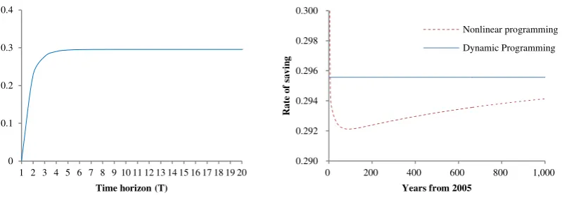
The left panel of Figure 1 shows the rate of saving for the problem of Equations (7) and (8),

calculated from Equation (15). As expected, longer time horizon increases the rate of saving.

The optimal rate of saving for the infinite time horizon problem (𝑇 → ∞) is 0.295567. As

shown in the right panel of Figure 1, our dynamic programming method with the logarithmic

approximations produces exact solution (up to 16th decimal place), which is more precise

than nonlinear programming with finite time horizon. The inclusion of the other exogenous

Figure 1 The rate of saving (Left): analytical solutions (Right): numerical solutions. Dynamic programming

refers to the solutions obtained from the method of this paper. Only a constant and the capital stock are included

as arguments for the value function. The maximum tolerance level and the simulation length are set at 10-6 and 1,000, respectively. Nonlinear programming refers to the solutions obtained from CONOPT (nonlinear

programming) in GAMS (time horizon 1,000 years). For numerical simulations, the initial value of the capital

stock and the evolutions of exogenous variables are drawn from DICE 2007.

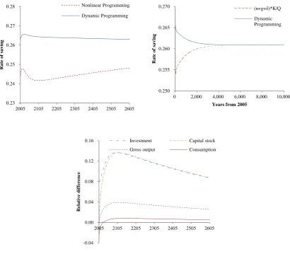
Applying 𝛿𝑘=0.1 and 𝛼=2, the rate of saving is higher for the dynamic programming than

for the nonlinear programming with finite time horizon. Put differently, optimal investment is

higher for the dynamic programming (see the top left panel of Figure 2). One of the reasons is

that the dynamic programming solves the infinite time horizon problem, whereas the

nonlinear programming solves the finite time horizon model.

The rate of saving should satisfy the following equation at equilibrium:𝑠∞= (𝑛+𝑔+

𝛿)𝐾_∞⁄𝑄_∞, where ∞ denotes the variables at equilibrium, 𝑛 and 𝑔 are the growth rates of

labor force and the total factor productivity, respectively (for more on this, see Romer, 2006).

The top right panel of Figure 2 shows that our dynamic programming finds the optimal path

that satisfies the relation at equilibrium.

The decision maker consumes less in the near future for the dynamic programming than for

the nonlinear programming. Such decisions produce more consumption in the future (more

0 0.1 0.2 0.3 0.4

1 2 3 4 5 6 7 8 9 10 11 12 13 14 15 16 17 18 19 20

R at e o f s avi n g (i n it ial ye ar )

Time horizon (T)

0.290 0.292 0.294 0.296 0.298 0.300

0 200 400 600 800 1,000

R at e o f s avi n g

Years from 2005

specifically, after 2028). The evolutions of the other variables including gross output, and the

capital stock depend on the behavior of the rate of saving (see the bottom panel of Figure 2).

Figure 2 The optimal solutions (the simple growth model) (Top): The rate of saving. (Bottom): The relative

difference between the dynamic programming and the nonlinear programming calculated as follows: (the results

of DP – the results of NP) / the results of DP. For dynamic programming, the maximum tolerance level and

simulation length are set at 10-6 and 1,000 years, respectively. For nonlinear programming time horizon is set at 1,000 years. 0.23 0.24 0.25 0.26 0.27 0.28

2005 2105 2205 2305 2405 2505 2605

R at e o f s avi n g Nonlinear Programming Dynamic Programming 0.250 0.255 0.260 0.265 0.270

0 2,000 4,000 6,000 8,000 10,000

R at e o f s avi n g

Years from 2005

(n+g+δ)*K/Q Dynamic Programming -0.04 0.00 0.04 0.08 0.12 0.16

2005 2105 2205 2305 2405 2505 2605

R el a ti v e d if feren ce

4 An Application: The DICE Model

Our solution method is applicable to more complex models such as the DICE model. The full

model is given in Appendix A. The Bellman equation and the basis function for this problem

are:

𝑊(𝒔_𝒕;𝒃) =𝑚𝑎𝑥

𝐶𝑡,𝜇𝑡[𝐿𝑡𝑈+𝛽𝑊(𝒔𝒕+𝟏;𝒃)] (16)

𝑊 ≈ 𝑏0+� 𝑏𝑖𝑙𝑛 (𝑠𝑖,𝑡)

𝑖=1

(17)

where µ𝑡 is the rate of GHG emissions control. Note that there are two control variables

(𝐶𝑡,𝜇𝑡) and six endogenous state variables (𝐾𝑡+1, 𝑀𝐴𝑇𝑡+1, 𝑀𝑈𝑡+1, 𝑀𝐿𝑡+1, 𝑇𝐴𝑇𝑡+1, 𝑇𝐿𝑡+1), where

𝑀𝐴𝑇𝑡+1, 𝑀𝑈𝑡+1, 𝑀𝐿𝑡+1 are the carbon stock in the atmosphere, the upper ocean, and the lower

ocean, respectively, 𝑇𝐴𝑇𝑡+1 and 𝑇𝐿𝑡+1 are air temperature changes and ocean temperature

changes (from 1900), respectively. Applying the first order conditions we get eight equations.

Arranging the first order conditions results in Equations (18) and (19) for optimal policy rules:

𝐵1,𝑡µ𝑡𝜃2+𝐵2,𝑡µ𝑡𝜃2−1+𝐵3,𝑡= 0 (18)

where

𝐵1,𝑡=−𝜃1,𝑡_𝐾𝑏1 𝑡

𝜁3

𝑀𝐴𝑇𝑡

�1− 𝜉₄�𝑄_𝑡𝛺_𝑡′

�1− 𝜉₄��𝜁₁𝑓+𝜁₂�− 𝜉₄𝜁₄+𝜃1,𝑡(𝜃2−1)𝑄𝑡𝛺𝑡 ′_� 𝑏2

𝑀𝐴𝑇𝑡

− 𝑃𝑡� (18-1)

𝐵2,𝑡=−𝜃1,𝑡(𝜃2−1)𝑄𝑡′𝛺𝑡�

𝑏2

𝑀𝐴𝑇𝑡

− 𝑃𝑡�+𝜃1,𝑡𝜃2

𝑏1

𝐾𝑡

𝛺𝑡

𝐵3,𝑡=_𝐾𝑏1 𝑡

𝜁3

𝑀𝐴𝑇𝑡

(1− 𝜉₄)𝑄_𝑡𝛺_𝑡′

(1− 𝜉₄)(𝜁₁𝑓+𝜁₂)− 𝜉₄𝜁₄−{(1− 𝛿𝑘) +𝑄𝑡

′_𝛺 𝑡}�_𝑀𝑏2

𝐴𝑇𝑡

− 𝑃𝑡� (18-3)

𝑃𝑡=_𝛿 𝛿𝑈𝐴

𝑈𝐿𝛿𝐿𝑈− 𝛿𝐿𝐿𝛿𝑈𝑈�

𝛿𝑈𝐿𝑏4

𝑀𝐿𝑡

−𝛿_𝑀𝐿𝐿𝑏3

𝑈𝑡

�+ 𝜁3 𝑀𝐴𝑇𝑡

�(1− 𝜉4)𝑏5

𝑇𝐴𝑇𝑡 − 𝜉

4𝑏6

𝑇𝐿𝑡 �

(1− 𝜉₄)(𝜁₁𝑓+𝜁₂)− 𝜉₄𝜁₄

(18-4)

(𝐶_𝑡⁄𝐿_𝑡)−𝛼=𝑏₁/𝐾_𝑡{(1− 𝛿_𝑘) +𝑄_𝑡′𝛺_𝑡(1− 𝛬_𝑡)−(1− 𝜇_𝑡)𝑄_𝑡′𝛺_𝑡𝛬_𝑡′}−1 (19)

where 𝛺𝑡 is the damage function, 𝛬𝑡 is the abatement cost function, 𝜁1=𝜉1𝜂/𝜆0, 𝜁2= 1− 𝜁1,

𝜁3=𝜉1𝜂/ln (2), 𝑓= 1− 𝜆0⁄𝜆, 𝑄𝑡′=𝜕𝑄𝑡⁄𝜕𝐾𝑡, 𝛺𝑡′=𝜕𝛺𝑡⁄𝜕𝑇𝐴𝑇𝑡 , 𝛬𝑡′ =𝜕𝛬𝑡⁄𝜕𝜇𝑡, and 𝑃0=𝛿𝐴𝐴+

𝛿𝑈𝐴𝛿𝐴𝑈𝛿𝐿𝐿/(𝛿𝑈𝐿𝛿𝐿𝑈− 𝛿𝐿𝐿𝛿𝑈𝑈). See Appendix A for notations and the parameter values.

Since the model is highly nonlinear and subject to irreversibility constraint (0≤ µ_𝑡 ≤1),

numerical methods for finding solutions are applied. More precisely, Newton’s method with

Fisher’s function for the root-finding problem is applied (Judd, 1998; Miranda and Fackler,

2004).

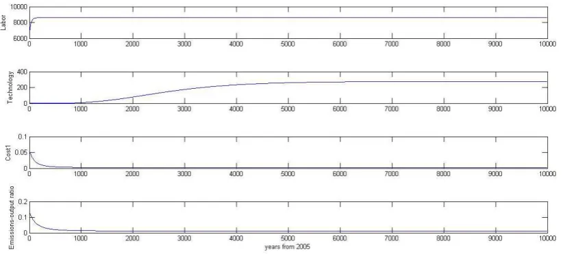
As shown in Figure 3, our solution method finds equilibrium far in the future. This is

because of the evolutions of the exogenous variables of the DICE model as shown in Figure 4.

With various experiments it is found that the simulation length larger than 1,000 does not

Figure 3 The optimal solutions (the DICE model) The units for consumption and the capital stock are

1,000US$/person. The units for the carbon stock and air temperature are GtC and °C, respectively.

Figure 4 The evolutions of the exogenous variables (the DICE model) Labor, technology, cost1, and

emissions-output ratio refer to 𝑳_𝒕, 𝐀_𝒕, 𝜽_𝟏,𝒕, and 𝝈𝒕, respectively.

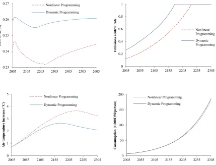
Similar to the simple growth model, the rate of saving (in turn, investment and gross output)

As a result, (business as usual) greenhouse gas emissions are higher for the dynamic

programming than for the nonlinear programming. This raises the rate of emissions control

for the dynamic programming compared to the nonlinear programming (in turn, lower

optimal temperature increases). Except for near future (until 2037), consumption is higher for

the dynamic programming than for the nonlinear programming.

Figure 5 The optimal solutions (the DICE model) (Top Left): The rate of saving (Top Right): The rate of

emissions control (Bottom Left): .Atmospheric temperature increases (from 1900) (Bottom Right):

Consumption

As shown in Figure 3, the rate of saving does not change much over time. In addition, the

rate of saving does not change much over time over a various plausible range of the climate

0.23 0.24 0.25 0.26 0.27

2005 2105 2205 2305 2405 2505 2605

R at e o f s avi n g Nonlinear Programming Dynamic Programming 0 0.2 0.4 0.6 0.8 1

2005 2055 2105 2155 2205 2255 2305

E m is si on s c on tr ol r a te Nonlinear Programming Dynamic Programming 0 1 2 3 4 5

2005 2055 2105 2155 2205 2255 2305

A ir t em p era tu re in crea se (° C) Nonlinear Programming Dynamic Programming 0 50 100 150 200

2005 2055 2105 2155 2205 2255 2305

C o n su m p ti on ( 1, 000U S $/ p er so n

) Nonlinear Programming

sensitivity. For instance, the rate of saving (defined as the gross investment divided by the net

production) changes in the range of 0.240 and 0.247 for the first 600 years in the DICE-CJL

model (Cai et al., 2012a), which is a modified version of DICE with an annual time step. For

instance, if the savings’ rate is fixed at 0.245 all variables including the optimal carbon tax

deviate only less than 3% from the original results. This holds even if the true value of the

climate sensitivity is set at 25°C/2xCO2.

Fixing the savings’ rate as in the model of Solow (1956) helps reduce computational

burden since the number of control variables is reduced. Furthermore fixing the savings’ rate

does not affect the optimal solutions much. For instance, the solutions of the reduced DICE

2007 model (fixing the savings’ rate at constant) obtained from dynamic programming are

compared with the results obtained from nonlinear programming in GAMS (i.e., using the

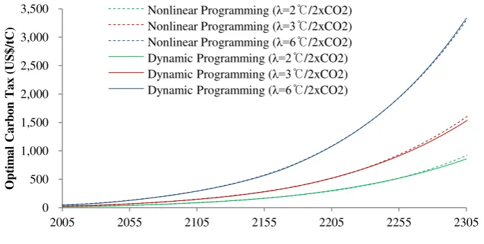
original programming code made available by William Nordhaus) in Figure 6, which shows

that our solution method produces almost the same results as the results from nonlinear

programming.

Figure 6 The optimal carbon tax 𝛌 refers to the equilibrium climate sensitivity. 0 500 1,000 1,500 2,000 2,500 3,000 3,500

2005 2055 2105 2155 2205 2255 2305

O p ti m al C ar b on T ax ( U S $ /t C )

The accuracy of the dynamic programming method is tested as follows. The maximum

welfare over a grid of the control variables is calculated for every time period. More

specifically, the model is simulated with a fixed emissions control rate (1,000 grid points

from 0 to 1) and then the rate of emissions control which results in maximum welfare is

chosen for every time period. The emissions control rate obtained above and the emissions

control rate obtained from the dynamic programming method are compared. The result is that

the maximum difference between the two values over the whole time periods is about 10-4.

5 Concluding Remarks

This paper develops a numerical method for solving a climate economy model. Our method

produces exact solutions to an (analytical) economic growth model and is useful for solving

more demanding models such as DICE. Only the Bellman equation, arguments of the value

function, and the first order conditions should be changed according to models. For instance,

Hwang et al., (2013, 2014) solve uncertainty and learning models on climate change having

up to 9 endogenous state variables with the method of this paper.

From the applications of our method, we find that optimal investment is calculated to be

slightly higher for the dynamic programming than for the nonlinear programming with finite

time horizon. Such decisions induce slightly lower near future consumption but higher

consumption in the future (after about 20-30 years) for the dynamic programming than for the

nonlinear programming. The optimal rate of emissions control (in turn, the optimal level of

temperature increases) is affected by the investment decision. More specifically, the decision

maker increases the rate of emissions control compared to the nonlinear programming and

Acknowledgements

The author is grateful to David Anthoff, Frederic Reyenes, and Richard S.J. Tol for valuable

comments on the earlier version of this paper. All remaining errors are the author’s.

References

Bellman, R. and Dreyfus, S.E., 1962. Applied dynamic programming. The RAND

Corporations.

Cai, Y., Judd, K.L., and Lontzek. T.S., 2012a. Open Science is Necessary. Nature Climate

Change 2(5), 299.

Cai, Y., Judd, K.L., and Lontzek, T.S., 2012b. DSICE: A dynamic stochastic integrated

model of climate and economy. The Center for Robust Decision Making on Climate and

Energy Policy Working Paper No. 12-02.

Hennlock, M. 2009. Robust control in global warming management: An analytical dynamic

integrated assessment. RFF Discussion Paper No. 09-19 University of Gothenburg.

Hwang, I.C., Tol, R.S.J., and Hofkes, M., 2013. Active learning about climate change. Sussex

University Working Paper Series No. 65-2013.

Hwang, I.C., Reynes, F., and Tol, R.S.J., 2014. The effect of learning on climate policy under

fat tailed uncertainty. MPRA working paper No. 53681.

Judd, K.L., 1998. Numerical methods in economics. The MIT press, Cambridge, MA, US.

Judd, K.L., Maliar, L., and Maliar, S., 2011. Numerically stable and accurate stochastic

simulation approaches for solving dynamic economic models. Quantitative Economics 2,

Kelly, D.L. and Kolstad, C.D., 1999. Bayesian learning, growth, and pollution. Journal of

Economic Dynamics and Control 23, 491-518.

Kelly, D.L., and Tan, Z., 2013. Learning and Climate Feedbacks: Optimal Climate Insurance

and Fat Tails. University of Miami Working Paper.

Lemoine, D., and Traeger, C., 2014. Watch Your Step: Optimal Policy in a Tipping Climate,

American Economics Journal: Economic Policy (forthcoming).

Leach, A.J., 2007. The climate change learning curve. Journal of Economic Dynamics and

Control 31, 1728-1752.

Maliar, L., and Maliar, S., 2005. Solving nonlinear stochastic growth models: iterating on

value function by simulations. Economics Letters 87, 135-140.

Miranda, M.J., and Fackler, P.L., 2004. Applied computational economics and finance. The

MIT Press, Cambridge, MA, US.

Nordhaus, W.D., 2008. A Question of Balance: Weighing the Options on Global Warming

Policies. Yale University Press, New Haven and London.

Roe, G.H., and Baker, M.B., 2007. Why is climate sensitivity so unpredictable? Science

318(5850), 629-632.

Romer, D., 2006. Advanced macroeconomics. McGraw-Hill/Irwin, New York.

Rust, J., 1996. Numerical dynamic programming in economics. Handbook of computational

economics 1, 619-729.

Solow, R.M.. 1956. A contribution to the theory of economic growth. The Quarterly Journal

Stocky, N.L., and Lucas, R.E., 1989. Recursive Methods in Economic Dynamics. Harvard

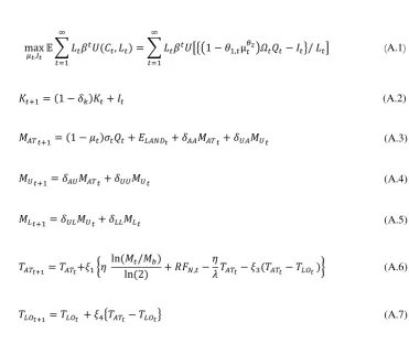
Appendix A: The Full Model

max

𝜇𝑡,𝐼_𝑡 𝔼 � 𝐿𝑡𝛽

𝑡_𝑈(𝐶 𝑡,𝐿𝑡) ∞

𝑡=1

=� 𝐿_𝑡𝛽𝑡𝑈���1− 𝜃₁,𝑡µ𝜃𝑡2�𝛺𝑡𝑄𝑡− 𝐼𝑡�/ 𝐿𝑡�

∞

𝑡=1

(A.1)

𝐾𝑡+1= (1− 𝛿𝑘)𝐾𝑡+𝐼𝑡 (A.2)

𝑀_{𝐴𝑇𝑡+1}= (1− 𝜇_𝑡)𝜎_𝑡𝑄_𝑡+𝐸_{𝐿𝐴𝑁𝐷𝑡}+𝛿_𝐴𝐴𝑀_𝐴𝑇𝑡+𝛿_𝑈𝐴𝑀_𝑈𝑡 (A.3)

𝑀_𝑈𝑡+1=𝛿_𝐴𝑈𝑀_𝐴𝑇𝑡+𝛿_𝑈𝑈𝑀_𝑈𝑡 (A.4)

𝑀_𝐿𝑡+1=𝛿_𝑈𝐿𝑀_𝑈𝑡+𝛿_𝐿𝐿𝑀_𝐿𝑡 (A.5)

𝑇𝐴𝑇𝑡+1=𝑇𝐴𝑇𝑡+𝜉1�𝜂

ln (𝑀_𝑡/𝑀_𝑏)

ln (2) +𝑅𝐹𝑁,𝑡−

𝜂

𝜆 𝑇𝐴𝑇𝑡− 𝜉3(𝑇𝐴𝑇𝑡− 𝑇𝐿𝑂𝑡)� (A.6)

𝑇𝐿𝑂𝑡+1=𝑇𝐿𝑂𝑡 +𝜉4�𝑇𝐴𝑇𝑡− 𝑇𝐿𝑂𝑡� (A.7)

where 𝔼 is the expectation operator, 𝑡 is time (annual). Notations, initial values, and

parameter values are given in Tables (A.1) and (A.2).

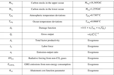
Table A.1 Variables

Variables Notes

U Utility function =(𝐶_𝑡⁄𝐿_𝑡)1−𝛼⁄(1− 𝛼)

𝐶𝑡 Consumption =�1− 𝜃1,𝑡µ𝑡𝜃2�𝛺𝑡𝑄𝑡− 𝐼𝑡

µ_𝑡 Emissions control rate Control variable

𝐼𝑡 Investment in general Control variable

𝐾𝑡 Capital stock 𝐾0=$137 trillion

𝑀_𝑈𝑡 Carbon stocks in the upper ocean 𝑀_𝑈0=18,365GtC

𝑀_𝐿𝑡 Carbon stocks in the lower ocean 𝑀_𝐿0=1,255GtC

𝑇𝐴𝑇𝑡 Atmospheric temperature deviations 𝑇𝐴𝑇0=0.7307°C

𝑇𝐿𝑂𝑡 Ocean temperature deviations 𝑇𝐿𝑂0=0.0068°C

𝛺𝑡 Damage function =1/(1 +𝜅1𝑇𝐴𝑇𝑡+𝜅2𝑇𝐴𝑇2𝑡)

𝑄𝑡 Gross output =𝐴𝑡𝐾𝑡𝛾𝐿1−𝛾𝑡

𝐴𝑡 Total factor productivity Exogenous

𝐿𝑡 Labor force Exogenous

𝜎𝑡 Emission-output ratio Exogenous

𝑅𝐹𝑁,𝑡 Radiative forcing from non-CO2 gases Exogenous

𝐸𝐿𝐴𝑁𝐷𝑡 GHG emissions from non-energy consumption Exogenous

𝜃1,t Abatement cost function parameter Exogenous

Note: The initial values for the state variables and the evolutions of the exogenous variables follow Nordhaus

(2008).

Table A.2 Parameters

Parameters Values

𝜆 Equilibrium climate sensitivity =𝜆₀/(1-𝑓)

𝑓 Total feedback factors 0.6

𝜆0 Reference climate sensitivity 1.2°C/2xCO2

𝛼 Elasticity of marginal utility 2

𝛽 Discount factor =1/(1 +𝜌)

𝜌 Pure rate of time preference 0.015

𝛾 Elasticity of output with respect to capital 0.3

𝛿𝑘 Depreciation rate of the capital stock 0.1

𝜅1, 𝜅2 Damage function parameters 𝜅1=0, 𝜅2=0.0028388

𝜃2 Abatement cost function parameter 𝜃2=2.8

𝛿𝑈𝑈, 𝛿𝑈𝐿, 𝛿𝐿𝐿,

𝜉1, 𝜉3, 𝜉4, 𝜂

𝛿𝐴𝑈=0.0097213, 𝛿𝑈𝑈=0.005,

𝛿𝑈𝐿=0.0003119, 𝛿𝐿𝐿=0.9996881,

𝜉1=0.022, 𝜉3=0.3, 𝜉4=0.005, 𝜂=3.8

𝑀𝑏 Pre-industrial carbon stock 596.4GtC

Note: The parameter values are from Nordhaus (2008) and Cai et al. (2012a) except that 𝜆₀ follow Roe and