The variance minimizing hedge with put options

The variance-minimizing hedge with put

options

Bell, Peter N

University of Victoria

15 November 2014

Running head: VARIANCE MINIMIZING HEDGE WITH PUT OPTIONS 1

© Peter Bell, 2014

The variance-minimizing hedge with put options

Peter N. Bell

Department of Economics, University of Victoria

Author note

Contact information: pnbell@uvic.ca, 250 588 6939.

Abstract

Certain commodity producers face uncertain output and price, but can trade financial derivatives

on price. I consider how best to use a put option on price. I introduce the variance surface,

which is a data visualization technique that shows the level of variance across a grid of values for

the two choice variables, quantity of options and strike price. The variance-minimizing hedge

has strike deep in the money and optimal quantity close to expected output, but the variance

surface shows there are near-best choices that are less expensive.

Keywords: Variance-minimizing hedge, put option, simulation, data visualization.

VARIANCE MINIMIZING HEDGE WITH PUT OPTIONS 3

The variance-minimizing hedge with put options

1. Introduction

Wheat farmers and gold miners both face a unique circumstance where the quantity and price

of their output is uncertain, but they can trade financial derivatives on price. Such producers face

a risk management problem with multiple sources of uncertainty. I use simulation to explore a

basic version of this problem: how to use put options on price to minimize the variance of

revenue. I use a brute force search algorithm to identify the optimal quantity of options and

strike price, but I also use data visualization to show that there are second best positions that

receive most of the benefit of the optimal hedge at lower cost.

Research on risk management with multiple sources of uncertainty arguably begins in

agricultural economics with McKinnon (1967), who uses the mean-variance framework to

analyze the optimal use of forward contracts. McKinnon finds that the optimal quantity of

forward contracts is equal to expected output when price and quantity are uncorrelated, less than

expected output under negative correlation, and greater than expected output under positive

correlation. Losq (1982) challenges these results with a general expected utility approach where

he shows it is optimal to hedge less than expected output whenever the third derivative of the

utility function is positive, which is associated with skewness preference. There is much further

debate on the topic in agricultural economics (Rolfo, 1980; Lapan & Moschini, 1994), but the

literature is generally limited to hedging with forward contracts.

Brown and Toft (2002) show how to go beyond basic forward contracts in a model where

risk management affects firm value. Brown and Toft’s model allows the producer to design an

distress costs. Oum and Oren (2010) demonstrate how to create an exotic derivative in the

mean-variance framework. Exotic derivatives allow the producer to customize the entire payoff

function, which is a sophisticated problem in functional analysis that generally requires a

numerical solution.

Although the literature covers forward contracts and exotic derivatives, there has been little

attention given directly to put options. This may be because put options are a special case of

exotic derivatives: the optimal exotic derivative must be at least as good as the optimal put

option. Although exotic derivatives are superior, they require some sophistication from the

producer to implement because they are not exchange traded. In contrast, put options are

exchange traded and the producer faces a relatively simple optimization problem with two

variables, quantity of options and strike price.

Since a position in put options is characterized by two variables, I use a data visualization

technique to assist with identification of the optimal put option. Data visualization is an

important part of research and practice in finance (Lemieux, 2013). I refer to the visualization as

the variance surface because it shows level sets of variance across option parameters. I use it to

identify the variance-minimizing hedge, show that the minimum is well defined, and explore

near-best options.

2. Simulation Experiment

2.1 Data Generating Processes

The probability model for quantity of output Q and price P are described by Equation (1), (2),

VARIANCE MINIMIZING HEDGE WITH PUT OPTIONS 5

normal distribution, but the quantity is normal and the price is lognormal. This does not yield an

immediate analytic solution, but it can be analyzed with simulation.

( 1 ) Q = Q0+ DQ .

( 2 ) P = P0e x p ( DP) .

( 3 ) [ DP, DQ] ~ N (μ,Σ)

The following parameters are fixed throughout the analysis. The initial quantity is one,

Q0=1, and price one hundred, P0=100. The change in price and quantity both have zero mean,

μ=[0,0]. The variance of change in price is constant throughout, Σ1,1=σP2 with σP=0.1. I

calculate the variance with different put options based on a large sample of observations, n=106,

from the joint distribution of [DP, DQ].

I vary other parameters to explore sensitivity of the results. The variance in quantity,

Σ2,2=σQ2, represents unhedged risk. I report results for a small level of unhedged risk, σQ=0.01,

and a large level, σQ=0.05. The covariance between change in quantity and price is Σ1,2=ρσPσQ.

The correlation, ρ, represents whether output provides a natural hedge on price (ρ<0) or not

(ρ>0). I report results for negative, zero, and positive correlation, ρ=-0.5, 0.0, or +0.5.

I use the Black Scholes formula for the option premium, as in Equation (4) and (5). The

premium, O(k), depends on strike price, k. I assume the interest rate is zero, r=0, and the option

expires after one time step, τ=1, to reflect a static trading strategy in the put option.

( 4 ) d1=(1/σP√τ)( l o g ( S0/ k ) + ( r + ½σP2)τ) , d2= d1-σP√τ.

( 5 ) O ( k ) = k e-r τΦ(- d2)–S0Φ(- d1) .

I calculate net revenue, N(q,k), as in Equation (6). The probability distribution of net

( 6 ) N ( q , k ) = P Q + q ( m a x [ k - P , 0 ] - O ( k ) er τ) .

I calculate the variance of net revenue, V(q,k), as in Equation (7).

( 7 ) V ( q , k ) = V a r ( N ( q , k ) )

I use a brute force search for to identify the variance-minimizing hedge. I define the search

set as S=q x k, where q={0, 0.02, …, 2} and k={50, 51, …,150}, which is chosen to cover the

range of possible values for price and quantity of output. I calculate the variance V(q,k) at each

point in the search set based on the random sample of observations for [DP, DQ] and identify the

variance-minimizing hedge directly. I also use the search set to build the variance surface.

2.2 Variance Surface

Figure 1 shows the variance surface when price and quantity independent, ρ=0, and

unhedged risk is large, σQ=0.05. The axes are defined by the search set S and the height of the

VARIANCE MINIMIZING HEDGE WITH PUT OPTIONS 7

Figure 1 suggests that the variance surface is a convex function, which is a desirable property

because it suggests the minimizing hedge may be unique. My estimate of the

variance-minimizing hedge is, indeed, unique and it is also a corner solution: the variance-variance-minimizing

hedge has (q*,k*)=(1.00, 150) and V(q*,k*)=25.5. The quantity of options equals expected

output E(Q)=1 and the strike price is far above the initial price P0=100, which means the option

is deep in the money. Since this option is almost surely in the money, it functions like a forward

contract with artificially high forward price. This option is expensive because of high intrinsic

value and does not exploit the convexity of the put option payoff function.

Although the variance-minimizing hedge is unique, Figure 1 shows that many other put

the money, say k=110, and quantity larger than one, say q=1.2, will cause variance to equal

approximately 30. Such an option is similar to the variance-minimizing hedge but is less

expensive because it has lower intrinsic value.

2.3 Sensitivity Analysis

I report how the location of the variance-minimizing hedge changes with the level of

unhedged risk, σQ, and the size of correlation between quantity and price, ρ.

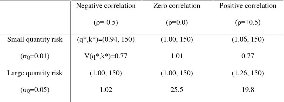
Table 1: Optimal quantity of put options, strike price, and variance of revenue

for different risk structures

Negative correlation (ρ=-0.5) Zero correlation (ρ=0.0) Positive correlation (ρ=+0.5)

Small quantity risk

(σQ=0.01)

(q*,k*)=(0.94, 150) V(q*,k*)=0.77 (1.00, 150) 1.01 (1.06, 150) 0.77

Large quantity risk

(σQ=0.05)

(1.00, 150) 1.02 (1.00, 150) 25.5 (1.26, 150) 19.8

Table 1 shows the optimal strike price is deep in the money across different risk structures,

but there are small changes in the optimal quantity of options. The optimal quantity of options

are in line with McKinnon (1967). The optimal quantity of options is slightly below expected

output when there is negative correlation between price and output because negative correlation

provides a natural hedge, which reduces the need for the put option. The optimal quantity of

options is slightly above expected output when there is positive correlation because positive

VARIANCE MINIMIZING HEDGE WITH PUT OPTIONS 9

3. Discussion

I find that the variance-minimizing put option generally has strike deep in the money, which

means it functions like a forward contract with very high forward price. It may be that the

optimal strike diverges to arbitrarily large values, which is unrealistic. It is possible to address

this unrealistic problem by including a volatility smile in option pricing, where tail options have

higher prices than used in this paper. Volatility smile would not change the variance of revenues

because the option premium is constant, but volatility smile would decrease average revenue; a

researcher could explore how the optimal hedge changes with volatility smile by using a

mean-variance utility surface, rather than the mean-variance surface.

Although I identify the variance-minimizing hedge, the variance surface shows that other

options do nearly as well. This demonstrates the value of visual analytics and exploratory data

analysis over a blind faith in an optimal solution. More can be done with data visualization in

this setting, such as calculating different types of surfaces. For example, the mean-variance

utility surface mentioned above. It is also possible to use animations of the surface to further

explore the parameter space of the model. For example, an animation of the surface as

correlation range from -1 to +1 could reveal interesting structures in the results that are not

apparent in static analysis.

Acknowledgements

This research was supported by the Joseph-Armand Bombardier Canada Graduate Scholarship –

References

Adam, T.R. (2002). Risk Management and the Credit Risk Premium. Journal of Banking and

Finance, 26(2-3), 243—269.

Brown, G.W., & Toft, K.B. (2002). How Firms Should Hedge. The Review of Financial

Studies, 15(4), 1283—1324.

Feder, G. Just, R.E., & Schmitz, A. (1980). Futures Markets and the Theory of the Firm Under

Price Uncertainty. The Quarterly Journal of Economics, 94(2), 317—328.

Lapan, H., & Moschini, G. (1994). Futures hedging under price, basis, and production risk.

American Journal of Agricultural Economics, 76, 465—477.

Lemieux, V. (Ed.). (2013). Financial Analysis and Risk Management: Data Governance,

Analytics and Life Cycle Management. Berlin, Heidelberg: Springer-Verlag.

Losq, E. (1982). Hedging with price and output uncertainty. Economics Letters, 10, 65—70.

McKinnon, R.I. (1967). Futures Markets, Buffer Stocks, and Income Stability for Primary

Producers. Journal of Political Economy, 75(6), 844—861.

Oum, Y., & Oren, S.S. (2010). Optimal Static Hedging of Volumetric Risk in a Competitive

Wholesale Electricity Market. Decision Analysis, 7(1), 107—122.

Rolfo, J. (1980). Optimal Hedging under Price and Quantity Uncertainty: the Case of a Cocoa