Robustness and Stability of Limit Cycles in a Class of Planar Dynamical Systems

Munich Personal RePEc Archive

Robustness and Stability of Limit Cycles

in a Class of Planar Dynamical Systems

Datta, Soumya

Faculty of Economics, South Asian University

June 2014

Online at

https://mpra.ub.uni-muenchen.de/56970/

Robustness and Stability of Limit Cycles in a

Class of Planar Dynamical Systems

Soumya Datta

Faculty of Economics, South Asian University, New Delhi, INDIA. Email:[email protected]

June 29, 2014

Abstract

Using the Andronov-Hopf bifurcation theorem and the Poincar´e-Bendixson Theorem, this paper explores robust cyclical possibilities in a generalized Kolmogorov-Lotka-Volterra class of models with positive intraspecific cooperation in the prey population. This addi-tional feedback effect introduces nonlinearities which modify the cyclical outcomes of the model. Using an economic example, the paper proposes an algorithm to symbolically con-struct the topological normal form of Andronov-Hopf bifurcation. In case the limit cycle turns out to be unstable, the possibilities of the dynamics converging to another limit cycle is explored.

Keywords: Kolmogorov-Lotka-Volterra Model, predator-prey, Andronov-Hopf bifurcation, Limit cycles

JEL classification: C62; C69

∗_{Parts of this paper are drawn from the author’s Ph.D. thesis, titledMacrodynamics of Financing Investment:}

1. Introduction

Economic theory has long been engaged in attempts to explain persistent cyclical behavior of variables like income and investment, resulting in business and growth cycles. At least one line of investigation in this literature has been to look for endogenous deterministic explanations for such cycles. In this paper, we look at the possibilities of robust cyclical behavior in a class of planar dynamical systems which might be useful in this line of literature.

The specific class of planar dynamical systems which we are going to examine in this study consists of two variables with a two-way causality running between them. The Lotka-Volterra or the predator-prey class of models, originally formulated by Lotka (1925) and Volterra (1927) in a biochemical and ecological application respectively, and later on generalized by Kolmogorov (1936), Freedman (1980, chapter 5), Huang & Zhu (2005) and Mukherji (2005), is an example of this class of models. The possibility of this class of models lending itself to model eco-nomic phenomena was noticed by Goodwin (1967), Samuelson (1967), Samuelson (1971) and many others. In fact, Flaschel (2010) demonstrated that this class of models might be utilized in a very diverse set of macroeconomic problems to yield endogenously bounded and cycli-cal outcomes. However, as pointed out, among others, by Flaschel (1984), Mukherji (2005) and Datta & Mukherji (2010), robustness of the cyclical outcomes in these models might be a matter of concern. In this study, we place a slightly modified set of restrictions to the general-ized Kolmogorov-Lotka-Volterra class of models than the ones discussed in the abovementioned studies. We demonstrate that the modifications we make to the restrictions are economically meaningful in a wide class of models, and can lead us to a much more robust cyclical outcomes than the ones found in the literature.

A related subject of our study is the Andronov-Hopf bifurcation theorem, which has been widely used to establish existence of limit cycles in this line of literature.1 _{However, in addition}

to the existence conditions, the Andronov-Hopf bifurcation must satisfy the non-degeneracy condition in order to prevent the degeneration of these limit cycles.2

Further, the Andronov-Hopf bifurcation might either be supercritical or subcritical. As pointed out by Benhabib & Miyao (1981) and Kind (1999), these two possibilities might have different economic interpre-tations. The supercritical case corresponds to stable limit cycles surrounding an unstable fixed point, and hence might be interpreted as stylized business or growth cycles. The subcritical case, on the other hand, correspond to repelling closed orbit surrounding a fixed point which is still stable, and might be interpreted to be corresponding to the concept of corridor stability as developed by Leijonhufvud (1973). A meaningful economic analysis of these limit cycles, therefore, requires a test for both non-degeneracy and stability. While numerically testing an Andronov-Hopf bifurcation point for non-degeneracy and stability is quite widespread in the literature in natural sciences,3

a substantial literature in economics relies on symbolic compu-tation. This is one of the reasons why the literature in economics often stops short of testing

1_{See, for instance, Asada & Yoshida (2003), Asada, Chen, Chiarella & Flaschel (2006), Barnett & He}

(1998), Barnett & He (2006), Benhabib & Nishimura (1979), Benhabib & Miyao (1981), Chiarella & Flaschel (2000), Chiarella, Flaschel & Franke (2005), Franke (1992), Velupillai (2006) and Minagawa (2007).

2_{See, for instance, Kuznetsov (1997).}

3_{In fact, software packages like XPPAUT or MATCONT already incorporate some of the standard algorithms}

Andronov-Hopf bifurcation for non-degeneracy and stability.4

We attempt to address this con-cern in this paper. We use a method outlined by Kuznetsov (1997) and Edneral (2007) to

symbolically compute the topological normal form for an Andronov-Hopf bifurcation in plane and test for non-degeneracy and stability of its limit cycles. We also explore whether, under certain conditions, there is a possibility of alternate stable limit cycles emerging when the test for stability of the limit cycle from Andronov-Hopf bifurcation fails. It would be obvious that a positive answer to the above question will widen the scope for cyclical possibilities to emerge in this class of models.

We begin by providing an outline of the generalized Kolmogorov-Lotka-Volterra class of models and point out the specific restrictions which we modify. We then illustrate this with a simple example of such a dynamical system and examine the robustness of limit cycles emerging from such a system.

2. A Generalized Kolmogorov-Lotka-Volterra Model

We begin with a generalized formulation of the predator-prey or Kolmogorov-Lotka-Volterra class of models, in line with the ones found in Kolmogorov (1936), Freedman (1980, chapter 5), Huang & Zhu (2005) and Mukherji (2005). Consider an ecological environment consisting of two species, one of which (predator) preys on the other (prey). The population of the prey depends inversely on the population of the predator, while the population of the predator depends directly on the population of prey. This simple story, which formed the basis of the original Lotka-Volterra formulation5

is often augmented with additional features, like the problem of resource constraint or ‘overcrowding’6

, when the prey population feeds on a natural resource like grass. Growth of prey population leads to a shortage of this natural resource, which acts as a self-limiting factor. Similar problem of overcrowding also exists for the predator species.

We model the above story using two variables, xand y, and two continuously differentiable functionsM, N :_ℜ+× ℜ+ → ℜwith the following set of properties:

P1. M(0,0)>0, My(x, y)<0, Nx(x, y)>0 ∀(x, y)∈ ℜ+× ℜ+

P2. Ny(x, y)<0 ∀(x, y)∈ ℜ+× ℜ+

P3. N(0,0)>0, Mx(x, y)≥0 ∀x∈[0,xˆ], Mx(x, y)<0 otherwise, Mxx(x, y)<0

∀(x, y)_{∈ ℜ}+× ℜ+

In the terminology of the predator-prey class of models, x might be interpreted to represent the prey population, whereasymight be interpreted to represent the predator population. The dynamical system might be described by the following system of differential equations:

˙

x(t) =x(t)M(x(t), y(t)) (1a) ˙

y(t) =y(t)N(x(t), y(t)) (1b)

4_{Benhabib & Nishimura (1979), however, is an early notable exception.} 5_{See for instance Hirsch, Smale & Devaney (2004, chapter 11).}

Out of the restrictions imposed on the functions M and N, namely P1, P2 and P3, Mukherji (2005) contains a discussion of P1 and P2. Briefly, P1 comes from the basic Lotka-Volterra relationship between the predator and the prey species explained above, while P2 comes from the existence of ‘overcrowding’ in the predator species. P3, however, represents a modification to the model outlined in the existing literature on this class of models, and hence merits a more detailed discussion.

It might be noted that the restrictions included in P3 makes the function M nonlinear, un-like the conventional literature in this area where bothM and N are linear. Such nonlinearity might arise, for instance, due to two opposite forces simultaneously at work – one leading to a positive impact of x and other leading to a negative impact on itself. The latter might occur, as we already discussed above, due to the existence of a resource constraint (‘overcrowding’ or ‘social phenomenon’), or more generally, intraspecific competition. The former might occur due to a variety of reasons, for instance, in the context of predator-prey model, this might rep-resent gains from intraspecific (i.e. among the members of the prey species) cooperation and social networks. Examples of such an intraspecific cooperation could be the members of the prey species signalling each other regarding the impending danger of an approaching predator, or using various forms of social networks to defend themselves against the predator. We as-sume that at low population size of the prey species, the intraspecific cooperation dominates, resulting in a positive value ofMx(x, y). However,Mxx(x, y)<0, i.e. the intraspecific

compe-tition progressively gets stronger vis-a-vis intraspecific cooperation with an increase in the prey population, so that eventually, after a critical point ˆx, it starts dominating. Mx(x, y)<0

be-yond ˆx. The nonlinearities arising from introduction of intraspecific cooperation represent our main departure from the existing literature on generalized Kolmogorov-Lotka-Volterra class of models.

We should point out here that introduction of such nonlinearities due to intraspecific co-operation might widen the scope of possible economic applications of such models. Consider, for instance, a traditional Keynesian multiplier-accelerator model7

with financial dampeners. The basic real-financial interaction might be thought of as a predator-prey relationship – a real variable like, say, the rate of investment, might be thought of as the prey, while a suitably defined financial variable like the rate of interest8 _{or the level of indebtedness in the economy}9

might be thought of as a predator. An increase in the rate of investment typically results in a deterioration of financial variables, captured by either an increase in the rate of investment or an increase in the level of indebtedness, which in turn has a negative feedback effect on the rate of investment. These are captured by restrictions under P1. The basic multiplier-accelerator relationship (i.e. a positive impact of the rate of investment on itself from the demand side) might be captured by the intraspecific cooperation, while the negative impact from an increase in the rate of investment due to crowding out of either real or financial resources might be cap-tured by intraspecific competition (or ‘overcrowding’ or ‘social phenomenon’). Both these are contained in P3. For lower rates of investment, the positive feedback effect dominates; however,

7_{For instance, literature following early contributions made by Samuelson (1939) or Hicks (1950).} 8_{See, for instance, Datta (2011).}

beyond a critical rate of investment, the negative feedback starts dominating. In short, intro-duction of the positive feedback effect ofx onM(x, y) in the form of intraspecific cooperation allows us to model economic phenomena like the traditional Keynesian multiplier-accelerator relationship.

We should note here that positive feedback effect like the one resulting from a Keynesian multiplier-accelerator interaction (captured in our model as intraspecific cooperation), on its own, is typically destabilizing.10

We attempt to see a) the extent to which such interactions might be integrated with the rest of the literature on predator-prey Kolmogorov-Lotka-Volterra class of models, andb) whether robust cyclical possibilities exist in such modified Kolmogorov-Lotka-Volterra models.

Before proceeding with rest of our study, we introduce a specific economic example of such a model.

3. An Economic Application

Consider the dynamical system given below, representing the macroeconomic model devel-oped in Datta (forthcoming):

˙

g(t) = ha1g(t)−a2{g(t)} 2

−a3d(t) +a4 i

hg(t) ˙

d(t) = [b1g(t)−b2d(t) +b3]d(t)

(2)

whereg_∈[0, gmax] is the rate of investment (or the ratio of investment to capital stock),gmaxis

the maximum possible rate of investment11

dis the debt-capital ratio and a1, a2, a3, a4, b1, b2, b3∈

]0,_∞[ are composite parameters consisting of various combination of various behavioral pa-rameters. h is a control parameter. In the model in Datta (forthcoming), h represented the speed of adjustment of actual to the desired rate of investment; more generally, this might be interpreted as a parameter representing the speed of adjustment of the variableg.12

We note that the dynamical system represented by (2) satisfies all the conditions listed under P1, P2 and P3 in section 2 above.

We note that the dynamical system represented by (2) has six steady states, which we refer to asEi ¯gi,d¯i

,i_∈[0,1]. A full list of these steady states is provided in appendix A. We further note that at most two of these steady states, E5 ¯g5,d¯5

and E6 ¯g6,d¯6

, are economically meaningful, i.e. lies within real positive orthant. We further note the following:

Lemma 1. For the dynamical system represented by (2), the real positive orthant is invariant.

Proof. Provided in appendix B.

10_{Consider, for instance, Hicks (1950) – the model had to rely on exogenous ceilings and floors to explain}

turnarounds in business cycles.

11_{In other words,g}

max represents resource constraint commonplace in economic models.

12_{cf. Datta (forthcoming) for details and derivation of this model; however, these details, however, are not}

It follows from lemma 1 that since only dynamics strictly within the real positive orthant is economically meaningful, we focus our attention on only such trajectories and ignore other trajectories in the rest of our discussion. In other words, we only consider E5 and E6 for

discussion, and do not discuss the other steady states in the rest of this study.

Next we turn our attention to the trajectories starting from an initial point inside the real positive orthant. Depending on the configuration of parameters, we can list four different possibilities exhibiting qualitatively different dynamics. These four cases are illustrated in figure 1. Details of parametric conditions giving rise to these four cases are discussed in appendix C.

Figure 1: Phase diagram of (2): Four cases

4. Andronov-Hopf Bifurcation

Lemma 2. For an appropriate value of the speed of adjustment, h, of the actual rate of investment to its desired rate, the characteristic equation to (2) evaluated at the non-trivial steady state, E6, has purely imaginary roots.

Proof. Consider the trace of the jacobian of the right hand side of (2), evaluated at E6, and

recall that for case 1 of figure 1, ¯g6 >0, ¯d6 >0 and a1−2a2g¯6 >0, so that

∂(Trace)

∂h = (a1−2a2g¯6) ¯g6 >0 (3)

i.e. the trace is smooth, differentiable and monotonically increasing in the speed of adjustment,

h, of the actual to the desired rate of investment. We further note that the trace disappears at h= ˆh, when

(a1−2a2g¯6) ˆhg¯6−b2d¯6 = 0

⇒ ˆh= b2d¯6 (a1−2a2g¯6) ¯g6

>0 (4)

which, by substituting the values of ¯g6 and ¯d6 from (7), might be expanded as

ˆ

h= b1b₂√4a₂b2

2a4−4a₂b₂a₃b₃₊b2

1a23−2a₁b₁b₂a₃₊a2

1b22+2a2b2

2b3−b2

1b2a₃₊a₁b₁b2

2 (2b

1a3−a1b2)√4a2b22a4−4a2b2a3b3+b21a23−2a1b1b2a3+a21b22−4a2b22a4+4a2b2a3b3−2b2₁a2₃₊₃a1b1b2a3−a2₁b2₂

(5)

We define ˆh as the critical value of the parameter, h, and investigate the properties of a solution trajectory to (2) around ˆh. Next, we apply the Andronov-Hopf Bifurcation Theorem to note the following:

Corollary 2.1. For the dynamical system represented by (2), h = ˆh provides a point of Andronov-Hopf bifurcation.

Proof. From lemma 2, the characteristic equation to (2) has purely imaginary roots ath= ˆh. Further, the transversality condition is satisfied from (3). Hence, h = ˆh provides a point of Andronov-Hopf bifurcation.

Lemma 3. For the dynamical system represented by (2), we can identify specific combination of parameter values for which the Andronov-Hopf bifurcation at h = ˆh is non-degenerate and supercritical (or subcritical), leading to emergence of unique and stable (or unique and unstable) limit cycles.

Proof. Provided in appendix D.

5. Global Stability Properties

We recall that for any (g◦_{, d}◦_)∈intℜ2

++as the initial point, the solution to (2) is represented

by Θ (t) = (g(t), d(t) ; g◦_{, d}◦_{). We attempt in this section to find out the behavior of this}

We define a set Q_⊆int _ℜ2

++ consisting of the rectangular area as follows:

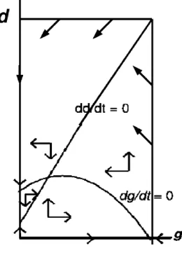
Q=_{(g, d) :g_∈[0,g¯3], d∈[0, dmax]} (6)

wheredmax= (b1/b2) ¯g3+ (b3/b2) =

b1 p

4a2a4+a21+ 2a2b3+a1b1

/(2a2b2). It would be

evident thatdmax is the point of intersection of ˙d/d= 0 with the vertical straight line g= ¯g3

(See figure 2).

Figure 2: Invariant setQ

We further defineQB ⊆Qcomprising the boundary ofQ, such thatQB={(g, d) :g= 0, d∈[0, dmax]} ∪

{(g, d) :g= ¯g3, d∈[0, dmax]} ∪ {(g, d) :g∈[0,g¯3], d= 0} ∪ {(g, d) :g∈[0,g¯3], d=dmax}.

Next, we note the following:

Lemma 4. For the trajectory Θ (t) = (g(t), d(t) ; g◦_{, d}◦_{), the set Q as defined in (6) is}

invariant.

Proof. Provided in appendix E.

Theorem 1. For any(g◦_{, d}◦_)∈intℜ2_{++, the trajectory,Θ (t)either approaches the non-trivial}

steady state, E6, or is a limit cycle surrounding it.

Proof. First, suppose (g◦_{, d}◦_{) ∈int Q. We recall that for case 1 of figure 1, E6 is the unique}

steady state in the interior of the positive orthant, and is either a source or a sink. Equations (4) and (5) provide us with a condition to distinguish between the two. In other words,h <ˆhwill imply thatE6is a sink; on the other hand, ifh >hˆ, then the steady stateE6is a source, so that

by Poincar´e-Bendixson Theorem there must be a limit cycle surroundingE6. Next, consider

(g◦_{, d}◦_)∈intℜ2

++\Q

. By construction, Θ (t) will eventually enterQ. Subsequently, it will either converge toE6 or will approach a limit cycle around E6. This completes the proof.

6. Multiple Limit Cycles

In section 4, we noted the emergence of limit cycle from Andronov-Hopf bifurcation. We further noted that this limit cycle could be either attracting or repelling, depending on the configuration of the parameters. In case of a subcritical Andronov-Hopf bifurcation leading to repelling or unstable limit cycle, if the limit cycle is located within an invariant set, then, from Poincar´e-Bendixson Theorem we have possibilities of another limit cycle which is attracting.13

Consider, for instance, the non-trivial steady state, E6, located within an invariant set, Q,

in figure 2. We recall that the steady state E6 is either a source or a sink, depending on

whether the value of the parameter, h, is greater than or less than the critical value, ˆh. We further note from corollary 2.1 that E6 undergoes a Andronov-Hopf bifurcation leading to

emergence of a small amplitude limit cycle when the bifurcation parameter, h passes through its critical value, ˆh. Let Γh be this limit cycle. Since Γh ∈ Q, it follows from the Jordan

curve theorem14

that Q is separated into two sets – a compact set, A(Γh), comprising the

area enclosed by Γh such that A(Γh) ⊆ Q, and, the half-open bounded set Q\A(Γh) ≡

{(g, d) : (g, d)_∈Q& (g, d)_∈/A(Γh)}. A(Γh) is bounded by Γh, the limit cycle resulting due

to Poincar´e-Andronov-Hopf bifurcation. Suppose further that the configuration of parameters is such that the Andronov-Hopf bifurcation is subcritical, so that Γh is repelling. Now we note

the following:

Lemma 5. Q_\A(Γh) is non-empty.

Proof. We recall that Q is a compact invariant set, bounded by QB, and that all trajectories

with an initial point on QB such that g, d 6= 0 gets pushed towards interior of Q. In other

words, QB cannot be the ω-limit set of any trajectory. Since Γh is a limit cycle, A(Γh) must

be a proper subset ofQ, so that Q_\A(Γh) is non-empty.

Lemma 6. ForΘ (t) = (g(t), d(t) ; g◦_{, d}◦_{), Q\A(Γ}

h) is invariant.

Proof. Consider a trajectory, Θ (t) starting from an initial point, (g◦_{, d}◦_{) ∈ Q\A(Γ}

h). We

have already established, from lemma 4 that for all (g◦_{, d}◦_{)∈Q the solution trajectory, Θ (t)}

cannot crossQB. We further note that, since Γh is repelling, for all (g◦, d◦)∈Q\A(Γh), Θ (t)

cannot cross Γh. SinceQ\A(Γh) is constructed on a plane, the solution needs to cross either

QB or Γh in order to leaveQ\A(Γh). Hence, Q\A(Γh) is invariant.

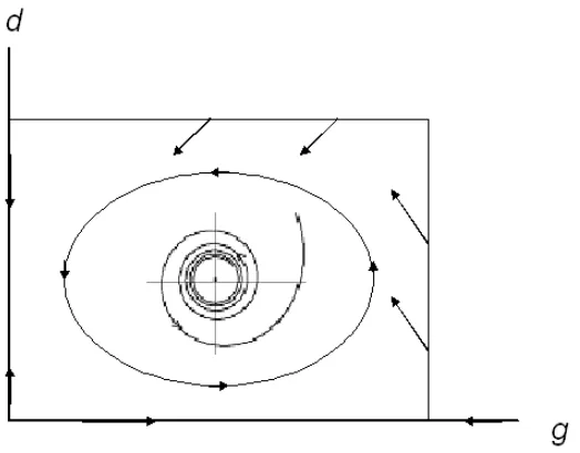
Theorem 2. If the steady stateE6 undergoes a subcritical Poincar´e-Andronov-Hopf bifurcation at the critical value of the bifurcation parameter, ˆh, then as the bifurcation parameter h passes throughhˆ, in addition to the small amplitude unstable limit cycle, Γh, there exists at least one large amplitude limit cycle which is attracting.

Proof. We note that, by construction,Q_\A(Γh) contains no locally stable fixed point. Hence,

from Poincar´e-Bendixson Theorem, for any (g◦_{, d}◦_{) ∈ Q\A(Γ}

h), ω-limit set of the solution

13_{See Hofbauer & So (1990), Hsu & Hwang (1999) and Yuquan, Zhujun & Chan (1999) for practical examples}

of emergence of multiple limit cycles by this method.

14_{The Jordan Curve Theorem. LetCbe a simple closed curve inS}2_{. ThenCseparatesS}2 _{precisely into two}

trajectory, Θ (t) will be a closed orbit. Further, the limit cycle, Γh, emerging from

Andronov-Hopf bifurcation as the bifurcation parameter passes through its critical value is not contained inQ_\A(Γh), i.e. Γh ∈/ Q\A(Γh). Hence, the ω-limit set of Θ (t) must be a large amplitude

limit cycle which is distinct from Γh. We further note that this large amplitude limit cycle is

attracting. (See figure 3)

Figure 3: A small amplitude unstable limit cycle surrounded by a large amplitude stable limit cycle

It is clear from theorem 2 that in case of a subcritical Andronov-Hopf bifurcation, the following two kinds of trajectories would emerge:

1. For any (g◦_{, d}◦_{) ∈ intA(Γh) the ω-limit set of the solution trajectories would be the}

steady state, E6. This behavior would be similar to Leijonhufvud’s (1973) notion of corridor stability.

2. For any (g◦_{, d}◦_)∈Q\A(Γ

h), theω-limit set of the solution trajectories would be a large

amplitude limit cycle.

In other words, a subcritical Andronov-Hopf bifurcation leads to possibilities of emergence of multiple limit cycles.

7. Conclusions

The above discussion leads us to the following conclusions:

1. For the dynamical system represented by (2), we define a critical value of the parameter

2. The limit cycle emerging from Andronov-Hopf bifurcation is either stable or unstable; in case it is unstable, from theorem 2, we have another stable limit cycle enclosing the unstable limit cycle.

3. Forh >ˆh, from theorem 1, we have a stable limit cycle from an application of Poincar´e-Bendixson theorem.

In other words, given ˆh, we have established the existence of a unique stable limit cycle for all

h_≥ˆh. We should note that this result for existence of stable limit cycles is more robust than much of the current literature on Kolmogorov-Lotka-Volterra class of models.

Finally, we also point out that these results can be more generally applied to the broader class of economic applications of planar dynamical systems of the type described in section 2 and characterized by the restrictions imposed under P1, P2 and P3, where both Andronov-Hopf bifurcation theorem and Poincar´e-Bendixson theorem are applicable. Applicability of this method is not limited by other details of the model chosen in this study.

Appendix A

Steady states

The steady states of the dynamical system represented by (2) are as follows:

E1 : ¯g1,d¯1

= (0,0) (7a)

E2 : ¯g2,d¯2

=

− √₄

a2a4+a2₁−a1

2a2 ,0

(7b)

E3 : ¯g3,d¯3

=

√

4a2a4+a21+a1

2a2 ,0

(7c)

E4 : ¯g4,d¯4

=0,b3

b2

(7d)

E5 : ¯g5,d¯5

=

− √₄

a2b22a4−4a2b2a3b3+b21a23−2a1b1b2a3+a21b22+b1a3−a1b2

2a2b2 ,

−b1√4a2b22a4−4a2b2a3b3+b21a23−2a1b1b2a3+a21b22−2a2b2b3+b21a3−a1b1b2

2a2b22

(7e)

E6 : ¯g6,d¯6

=

√

4a2b22a4−4a2b2a3b3+b21a23−2a1b1b2a3+a21b22−b1a3+a1b2

2a2b2 ,

b1√4a2b22a4−4a2b2a3b3+b21a23−2a1b1b2a3+a21b22+2a2b2b3−b21a3+a1b1b2

2a2b2₂

(7f)

It would be evident that E2 ∈ ℜ/ 2++ since ¯g2 < 0. Hence we do not discuss E2 any further

in the following sections. Further, E3 and E4 are non-negative and lie on the g and d axis

respectively. Regarding E5 and E6, we note the following:

1. Whenever E5 and E6 are real and distinct, ˙d/d = 0 must intersect ˙g/g = 0 from above

at E5 and from below atE6. IfE5 andE6 are not distinct, then ˙d/d= 0 is a tangent to

˙

g/g= 0 at the point representing the unique non-trivial steady state.

2. a3b3 < a4b2 is a sufficient (though not necessary) condition for the non-trivial steady

3. Forg(t)_≥¯g3, we have ˙g(t)≤0 for alld(t)∈ ℜ+; in other words, if ¯g3≤gmax, then the

feasibility condition 0_≤g(t)_≤gmax is always satisfied.

Appendix B

Proof of Lemma 1

For any (g◦_{, d}◦_{) ∈ int ℜ}2

++ as the initial point, let the solution to (2) be represented by

Θ (t) = (g(t), d(t) ; g◦_{, d}◦_{). From (2), we can conclude the following about the behavior of}

trajectories in case the initial point is on one of the axes:

(a) ˙g >0, d˙= 0 _{∀ {}(g◦_{, d}◦_{) : g}◦_{∈]0,¯g3[, d}◦ _{= 0} as the initial point.}

(b) ˙g <0, d˙= 0_{∀ {}(g◦_{, d}◦_{) : g}◦_{∈]¯g3,∞[, d}◦ _{= 0} as the initial point.}

(c) ˙g= 0, d >˙ 0 _∀

(g◦_{, d}◦_{) : g}◦ _{= 0, d}◦ _∈0,d¯_{4 as the initial point.}

(d) ˙g= 0, d <˙ 0_∀

(g◦_{, d}◦_{) : g}◦ _{= 0, d}◦ _∈¯

d4,∞ as the initial point.

(8)

i.e. both theg-axis and the d-axis are trajectories. Since trajectories cannot cross each other, this would make the real positive orthant invariant, i.e. trajectories starting from an initial point in the real positive orthant will always remain within it.

Appendix C

Parametric conditions for four cases of Figure 1

For g, d₆= 0, from (2) we have

˙

g(t)_⋚0 _⇔ d(t)_R a1

a3

g(t)₋a2

a3 {

g(t)_}2+a4

a3

˙

d(t)_⋚0 _⇔ d(t)_R b1

b2

g(t) +b3

(9)

Depending on the configuration of parameters, we can list four different possibilities exhibiting qualitatively different dynamics:

1. Case 1: Here, a4b2−a3b3 >0, i.e. intercept of ˙g/g = 0 is greater than that of ˙d/d= 0,

and b1/b2 > (a1−2a2g¯6)/a3 > 0, i.e. ˙d/d = 0 intersects ˙g/g = 0 from below in the

positively sloped section of the latter curve. E6∈intℜ2++ is the only steady state in this

case inside the real positive orthant.

2. Case 2: Here, a4b2−a3b3 >0, i.e. intercept of ˙g/g = 0 is greater than that of ˙d/d= 0,

but unlike case 1, (a1−2a2g¯6)/a3 < 0 < b1/b2, i.e. ˙d/d = 0 intersects ˙g/g = 0 from

below in the negatively sloped section of the latter curve. E6 ∈ intℜ2++ is the unique

steady state inside the real positive orthant.

3. Case 3: Here, a4b2−a3b3 <0, i.e. intercept of ˙g/g= 0 is less than that of ˙d/d= 0, and

(a1−2a2¯g5)/a3 > b1/b2 > 0 > (a1−2a2¯g6)/a3, i.e. ˙d/d = 0 intersects ˙g/g = 0 from

below atE5 when the latter is sloping upward, and from above at E6 when the latter is

sloping downward. In this case, E5, E6 ∈intℜ2++, i.e. ˙d/d= 0 intersects ˙g/g = 0 twice

in the interior of the real positive orthant.

4. Case 4: Here, a4b2−a3b3 < 0, i.e. intercept of ˙g/g = 0 is less than that of ˙d/d = 0,

and, unlike case 3, E5, E6 ∈/ intℜ2++ so that there does not exist any steady state in

Appendix D

Proof of Lemma 3

In order to establish that this Andronov-Hopf bifurcation point is non-degenerate, and to determine the stability of the limit cycles emerging from this bifurcation, we reduce our dy-namical system represented by (2) to its topological normal form, using a method outlined by Edneral (2007), Wiggins (1990), Kuznetsov (1997) and Kuznetsov (2006).15

This consists of the steps given below:

1. We perform a linear transformation of coordinates from (g(t), d(t)) to the new plane, (x1(t), x2(t)) such that g(t) =x1(t) + ¯g6, and d(t) =x2(t) + ¯d6. With this shift, the

steady state, E6 : ¯g6,d¯6

is placed at the origin, and the dynamical system (2) can be represented as

˙

x1(t) = h h

−a2{x1(t)} 3

+a6{x1(t)} 2

+a5x1(t)−a3x1(t)x2(t)−a7x2(t) i

˙

x2(t) = b4x1(t) +b1x1(t)x2(t)−b5x2(t)−b3{x2(t)}

2 (10)

where

a5 =

2b1a3s1−a1b2s1−4a2b22a4+ 4a2b2a3b3−2b21a 2

3+ 3a1b1b2a3−a21b 2 2

2a2b22

a6 =−

3s1−3b1a3+a1b2

2b2

a7 =

a3 (s1−b1a3+a1b2)

2a2b2

b4 =

b1 b1s1+ 2a2b2b3−b21a3+a1b1b2

2a2b22

b5 =

b1s1+ 2a2b2b3−b21a3+a1b1b2

2a2b2

s1 = q

4a2b22a4−4a2b2a3b3+b21a 2

3−2a1b1b2a3+a21b 2 2

2. For the transformed dynamical system represented by (10), we take a Taylor series ex-pansion around the steady state represented by the origin. The resulting expression can be represented in matrix notation as

˙

X =A(h)X+F(X, h) (11)

where X =

x1

x2

is a column vector of the two variables, and A(h) is the jacobian

matrix so that A(h)X represents the linear part of the Taylor series expansion, i.e.

A(h) =

a5h −a7h

b4 −b5

(12)

andF(X, h) represents the non-linear terms of the Taylor series expansion, starting with at least quadratic terms, such thatF(X, h) =O _||x_{| |}2

+O _||x_{| |}3

+. . .

15_{We implement this method by writing a program, using computer algebra system Maxima (Version 5.21.1,}

3. Next, we calculate the eigenvalues,ϑ(h) andϑ(h) of the jacobian matrix,A(h) from (12):

ϑ(h), ϑ(h) = 1 2

(a5h−b5)± q

a2

5h2+ (2a5b5−4a7b4) +b25

so that real part of the eigenvalues is expressed as Reϑ(h) =a5h−b5. Further,

d(Reϑ(h))

dh h=0

=a5 >0

i.e.transversality condition is satisfied.

4. We now recalculate the critical value, ˆh, of the bifurcation parameter, h. This would correspond to the right hand side of (5), expressed in terms of the new parameters defined above. Thus, we have

ˆ

h= b5

a5

(13)

Substituting the value of ˆh from (13) into (12), we have the jacobian at the critical value of bifurcation parameter:

Aˆh=





b5 −

a7b5

a5

b4 −b5 

 (14)

Further, we have DeterminantAˆh = (b4b5a7)/a5 −b25. We define ω such that

ω2_{= DeterminantA}ˆ_{h. We now expressA}ˆ_{h from (14) in terms ofω.}

Aˆh=



 

b5 −

a7b5

a5

a5 b25+ω 2

a7b5 −

b5 



 (15)

The eigenvalues ofAˆhevaluated at the critical value of the bifurcation parameter can

now be expressed as ϑˆh, ϑhˆ=_±ıω.

5. We now calculate the eigenvector ofAˆh with respect toϑˆh and call itq, where

q =

ıa7b5ω+a7b25

a5ω2+a5b25

i.e. Aˆhq = ϑˆhq. It would be evident that eigenvector of Ahˆ with respect to

ϑˆh would beq, whereq is the complex conjugate of q, so thatAˆhq=ϑˆhq.

6. We next calculate AT ˆ_{h, the transpose ofA}ˆ_h:

AT ˆh=



 

b5

a5 b25+ω 2

a7b5

−a7b5

a5 −

b5 



We note that the eigenvalues ofAT_{ˆhwould be the same as those of Ahˆand might}

be represented asϑhˆand ϑˆh.

7. We next calculate the eigenvector of AT ˆ_{hwith respect to ϑ}ˆ_{hand call it p, i.e.}

p=





1

a7b5

ıa5ω−a5b5 



i.e. AT _{ˆhp =ϑˆhp. It would be clear that the eigenvector of A}T _{ˆh with respect}

to ϑˆh would bep, i.e.AT ˆ_hp=ϑˆ_hp.

8. We note that the scalar product of pand q is given by

hp, q_i= 2ıa7b

2

5ω−2a7b5ω2

b5+ıω

We next normalizep with respect toq by suitably transforming fromp to ˆp, so that the scalar product of ˆp and q is one, i.e. _hp, qˆ _i= 1. This can be achieved by multiplying the column vectorpwith the reciprocal of the conjugate of the scalar product ofpandq, i.e.

ˆ

p_≡p. 1

hp, q_i

This leaves us with the following:

ˆ

p=



 

ıω₋b5

2a7b5ω2+ 2ıa7b25ω

1

2a5ω2+ 2ıa5b5ω 



 (17)

We now note that_hp, qˆ _i= 1.

9. Next, we perform a complex linear transformation, z =_hp, xˆ _i so that x =zq+zq. We should note thatx=zq+zq _{⇔ h}p, xˆ _i=z_hp, qˆ _i+z_hp, qˆ _{i ⇔ h}p, xˆ _i=z [_∵hp, qˆ _i= 1, _hp, qˆ _i= 0]. The transformation from (x1, x2) tozmight be viewed as a combination of two

transfor-mations,y=T(h)xandz=y1+ıy2. It would be clear that the components (y1, y2) are

the coordinates of (x1, x2) in the real eigenbasis ofA(h) composed by (2Re q,−2Imq).

In this basis, the matrixA(h) has its canonical real (Jordan) form

J(h) =T(h)A(h)T−1_{(h) =}

Re ϑ(h) ₋ω(h)

ω(h) Re ϑ(h)

This complex linear transformation imposes a linear relationship between (x1, x2) and

the real and imaginary parts of z. With this transformation, the dynamical system represented by (10) is now reduced to a single differential equation:

˙

z=ϑ(h)z+g(z, z, h) (18)

To perform this transformation, we first represent the right hand side of (10) by

F1(x1, x2) andF2(x1, x2) respectively. Next, we make the following substitution:

x1 =zq1+wq1 = a7b25+a7b5ıω

z+ a7b25−a7b5ıω

w x2 =zq2+wq2 = a5b25+a5ω2

(z+w) (19)

It might be noted that in the substitution made above in (19), we introduce an addi-tional variable, w instead of z in order to simplify the implementation of the algorithm in a symbolic manipulation software like Maxima. (See, for instance, Kuznetsov 1997, page 103, footnote 5). Substituting from (19), we have

F1(zq1+wq1, zq2+wq2)

= b5

a5

−a3

ıa7b5ω+a7b 2 5

z+ a7b 2

5−ıa7b5ω

w a5ω 2

+a5b 2 5

(z+w)

−a7 a5ω 2

+a5b 2 5

(z+w)₋a2

ıa7b5ω+a7b 2 5

z+ a7b 2

5−ıa7b5ω

w 3

+a6

ıa7b5ω+a7b25

z+ a7b25−ıa7b5ω

w 2+a5

ıa7b5ω+a7b25

z

+ a7b25−ıa7b5ω

w

(20)

and

F2(zq1+wq1, zq2+wq2)

= ₋b2

a5ω2+a5b25

(z+w) 2+b1

ıa7b5ω+a7b25

z+ a7b25−ıa7b5ω

w

a5ω 2

+a5b 2 5

(z+w) ₋b5 a5ω 2

+a5b 2 5

(z+w) +b4

ıa7b5ω+a7b 2 5

z

+ a7b25−ıa7b5ω

w

(21)

We define a matrixF such that

F =

F1(zq1+wq1, zq2+wq2)

F2(zq1+wq1, zq2+wq2)

(22)

and a new complex-valued functionG(z, w) such that

G(z, w) =_hp, Fˆ _i (23)

whereGcan be calculated by a scalar multiplication of ˆp from (17) withF from (22).16

10. Next, we calculate theFirst Lyapunov Exponent,ℓ1

ˆ

has follows:

ℓ1

ˆ

h= 1

2ω2 Re ı

∂2_G

∂z2

z=0,w=0

∂2_G

∂z∂w

z=0,w=0

+ω ∂

3_G ∂z∂z∂w

z=0,w=0 !

(24)

The computer algebra system, Maxima, calculates the value of first Lyapunov exponent of our system as:

ℓ1

ˆ

h=₋ 1 2a2 5ω

3

b5 b25+ω 2

3a2a5a27b 2 5ω

2

+a3a5a6a7b25ω 2

−a3

5a7b1b2ω2

−a2 3a 2 5b 2 5ω 2

−a3a35b2b5ω2+ 2a45b 2 2ω

2

−2a2 6a

2 7b

4

5+a5a6a27b1b35+a 2 5a 2 7b 2 1b 2 5

+3a3a5a6a7b45−3a 3

5a7b1b2b25−a 2 3a

2 5b

4

5−a3a35b2b35+ 2a 4 5b 2 2b 2 5 (25)

11. Once we have calculated the value of theFirst Lyapunov Exponent from (25) and estab-lished that it is non-zero (i.e. non-degeneracy conditions are satisfied), we can reduce (18) to its topological normal form using a series of transformations, including an invertible parameter-dependent shift of complex coordinates, a linear time rescaling and a non-linear time reparametrization, and elimination of terms of degree greater than four from the Taylor series (cf. Kuznetsov 1997, page 94-100). In this case, (18) can be represented in the topological normal form as:

˙

y1

˙

y2

=

α ₋1

1 α

y1

y2

+̟ y21+y 2 2

y1

y2

(26)

where̟= signℓ1

ˆ

h=_±1,α= Re ϑ(h)

ω(h) ∈ ℜand y= (y1, y2)

T

∈ ℜ2

.

The normal form represented by (26) is locally topologically equivalent to the original dy-namical system represented by (2) near the steady state, E6. For̟ = +1, the normal form

has a steady state at the origin, which is asymptotically stable for α _≤ 0 and unstable for

α > 0; in the latter case, a unique and stable limit cycle with radius√α will emerge. This is the case of a supercritical Andronov-Hopf bifurcation. Similarly, for ̟ = ₋1, the normal form has a steady state at the origin, which is asymptotically stable for α < 0 and unstable forα _≥0; in the former case, a unique and unstable limit cycle will emerge. This is the case of asubcritical Andronov-Hopf bifurcation.

Appendix E

Proof of Lemma 4

Consider a trajectory Θ (t) starting from an initial point located on the boundary,QB ofQ,

i.e. (g◦_{, d}◦_{) ∈Q}

B. We recall from (8) that theg-axis and the d-axis are both trajectories. In

particular, sinceE1(0,0) is a steady state,

(g◦_{, d}◦_{) =E1(0,0)⇒Θ (t) =E1(0,0) ∀ t∈ ℜ (27)}

Since E3(¯g3,0) andE4 0,d¯4

are also steady states, by same logic,

(g◦_{, d}◦_{) =E3(¯g3,0) ⇒ Θ (t) =E3(¯g3,0) ∀ t∈ ℜ (28)}

(g◦_{, d}◦_{) =E}

4 0,d¯4

⇒ Θ (t) =E4 0,d¯4

∀ t_{∈ ℜ} (29)

In other words, if the initial point is either on E1, E2 or E3 then the trajectory will remain

at the initial point. Further, from (8), if the initial point is on either g-axis or d-axis, but not on one of the steady states, it will approach E3 and E4 respectively. On the other hand,

for (g◦_{, d}◦_{) ∈ {(g, d) :g= ¯g3, d∈]0, dmax[}, we have ˙g <0 and ˙d > 0 ; whereas for (g}◦_{, d}◦_{) ∈} {(g, d) :g_∈]0,g¯3[} we have ˙g < 0 and ˙d < 0; i.e. in both cases the trajectories would be

pushed towards interior of Q. To summarize, for any (g◦_{, d}◦_{) ∈ QB, the trajectories either}

remain onQB or are pushed towards the interior ofQ; in no case do the trajectories leave Q.

[See figure 2] In addition, sinceQis constructed on a plane, i.e. Q_{⊆ ℜ}2

++, no trajectory with

an initial point in the interior ofQcan leave Qwithout crossingQB. This completes the proof

References

Asada, T., Chen, P., Chiarella, C. & Flaschel, P. (2006), ‘Keynesian dynamics and the wage-price spiral: A baseline disequilibrium model’,Journal of Macroeconomics 28(1), 90–130.

Asada, T. & Yoshida, H. (2003), ‘Coefficient Criterion for Four-dimensional Hopf Bifurcations: A Complete Mathematical Characterization and Applications to Economic Dynamics’,

Chaos, Solitons and Fractals 18, 525–536.

Barnett, W. A. & He, Y. (1998), Bifurcations in Continuous-Time Macroeconomic Systems, Macroeconomics 9805018, EconWPA.

*http://ideas.repec.org/p/wpa/wuwpma/9805018.html

Barnett, W. & He, Y. (2006), Existence of Bifurcation in Macroeconomic Dynamics: Grand-mont was Right, Working papers series in theoretical and applied economics 200610, University of Kansas, Department of Economics.

*http://ideas.repec.org/p/kan/wpaper/200610.html

Benhabib, J. & Miyao, T. (1981), ‘Some New Results on the Dynamics of the Generalized Tobin Model’, International Economic Review 22(3), 589–96.

Benhabib, J. & Nishimura, K. (1979), ‘The Hopf Bifurcation and the Existence and Stability of Closed Orbits in Multisector Models of Optimal Economic Growth’, Journal of Economic Theory 21, 421–444.

Chiarella, C. & Flaschel, P. (2000), The Dynamics of Keynesian Monetary Growth: Macro Foundations, Cambridge University Press.

Chiarella, C., Flaschel, P. & Franke, R. (2005),Foundations for a Disequilibrium Theory of the Business Cycle: Qualitative Analysis and Quantitative Assessment, Cambridge University Press, Cambridge, U.K.

Datta, S. (2011), Investment-led growth cycles: A preliminary re-appraisal of Taylor-type mon-etary policy rules, inK. G. Dastidar, H. Mukhopadhyay & U. B. Sinha, eds, ‘Dimensions of Economic Theory and Policy: Essays for Anjan Mukherji’, Oxford University Press, New Delhi.

Datta, S. (forthcoming), Cycles and crises in a model of debt-financed investment-led growth,

in S. K. Jain & A. Mukherji, eds, ‘Perspectives on Efficiency, Growth and Inequality’, Routledge. working paper version at http://mpra.ub.uni-muenchen.de/50200/.

Datta, S. & Mukherji, A. (2010), Goodwin’s Growth Cycles: A Reconsideration, in B. Basu, B. K. Chakrabarti, S. R. Chakravarty & K. Gangopadhyay, eds, ‘Econophysics & Eco-nomics of Games, Social Choices and Quantitative Techniques’, Springer-Verlag Italia, pp. 263–276.

Flaschel, P. (1984), ‘Some stability properties of Goodwin’s growth cycle, a critical evaluation’,

Zeitschrift f¨ur National¨okonomie 44, 63–69.

Flaschel, P. (2010), Topics in Classical Micro- and Macroeconomics: Elements of a critique of Neoricardian Theory, Springer-Verlag, Berlin Heidelberg.

Franke, R. (1992), ‘Stable, Unstable and Persistent Cyclical Behavior in a Keynes-Wicksell Monetary Growth Model’, Oxford Economic Papers 44, 242–256.

Freedman, H. (1980), Deterministic Mathematical Models in Population Ecology, Marcel Dekker Inc., New York.

Goodwin, R. M. (1967), A Growth Cycle, in C. Feinstein, ed., ‘Socialism, Capitalism and Economic Growth: Essays Presented to Maurice Dobb’, Cambridge University Press, London, pp. 54–58. Revised version in: Hunt, E.K., Schwartz, J. (Eds.), A Critique of Economic Theory. Harmondsworth, UK: Penguin, 1972, pp. 442-449.

Hicks, J. (1950),A Contribution to the Theory of Trade Cycle, Oxford University Press, Lon-don.

Hirsch, M. W. & Smale, S. (1974), Differential Equations, Dynamical Systems, and Linear Algebra, Academic Press, Inc, New York.

Hirsch, M. W., Smale, S. & Devaney, R. L. (2004),Differential Equations, Dynamical Systems, and an Introduction to Chaos, Academic Press, San Diego, California.

Hofbauer, J. & So, J. W. H. (1990), ‘Multiple Limit Cycles for Predator-prey Models’, Math-ematical Biosciences 99(1), 71–75.

Hsu, S.-B. & Hwang, T.-W. (1999), ‘Hopf Bifurcation for a Predator-prey System of Holling and Leslie Type’,Taiwanese Journal of Mathematics 3(1), 35–53.

Huang, X. C. & Zhu, L. (2005), ‘Limit Cycles in a General Kolmogorov Model’, Nonlinear Analysis 60(8), 1393–1414.

Kind, C. (1999), ‘Remarks on the Economic Interpretation of Hopf Bifurcations’, Economics Letters 62, 147–154.

Kolmogorov, N. (1936), ‘Sulla Teoria di Volterra della Lotta per l’esistenza’, Giornelle dell’Istituto Italiano degli Attuari 7, 74–80.

Kuznetsov, Y. A. (1997),Elements of Applied Bifurcation Theory, Vol. 112 ofApplied Mathe-matical Sciences, second edn, Springer-Verlag, New York.

Kuznetsov, Y. A. (2006), ‘Andronov-Hopf bifurcation’,Scholarpedia 1(10), 1858. *http://www.scholarpedia.org/article/Andronov-Hopf bifurcation

Leijonhufvud, A. (1973), ‘Effective Demand Failures’,Swedish Journal of Economics75, 27–48.

Merton, R., ed. (1972), The Collected Scientific Papers of Paul A. Samuelson, Vol. III, The MIT Press, Cambridge, MA.

Minagawa, J. (2007), A determinantal criterion of Hopf bifurcations and its application to economic dynamics, in T. Asada & T. Ishikawa, eds, ‘Time and Space in Economics’, Springer, pp. 160–172.

Mukherji, A. (2005), Robustness of Closed Orbits in a Class of Dynamic Economic Models,in

S. Lahiri & P. Maiti, eds, ‘Economic Theory in a Changing World, Policy Modeling for Growth’, Oxford University Press, Delhi.

Munkres, J. R. (2000), Topology, second edn, Pearson Education, Inc.

Samuelson, P. A. (1939), ‘Interaction Between the Multiplier Analysis and the Principal of Acceleration’, Review of Economic Statistics(21), 75–78.

Samuelson, P. A. (1967), ‘A Universal Cycle?’,Operations Research-verfahren3, 307. Reprinted in Merton (1972), pp. 473-486.

Samuelson, P. A. (1971), ‘Generalized Predator-Prey Oscillations in Ecological and Economic Equilibrium’,Proceedings of the National Academy of Sciences68(5), 980–983. Reprinted in Merton (1972), pp. 487-490.

Velupillai, K. (2006), ‘A Disequilibrium Macrodynamic Model of Fluctuations’, Journal of Macroeconomics 28(4), 752–767.

Volterra, V. (1927), Variazioni e Fluttuazioni del Numero d’individui in Specie Animali Conviventi, in ‘Memorie del R. Comitato Talassografico Italiano’, Memoria CXXXI. Translated in: Applicable Mathematics of Non-Physical Phenomena, Oliveira-Pinto, F., Conolly, B.W., John Wiley & Sons, New York, 1982, pp. 23-115.

Wiggins, S. (1990),Introduction to Applied Nonlinear Dynamical Systems and Chaos, Springer-Verlag, New York, Inc.